
INTRODUCTION
The domestic market represents a great proportion of tourism demand in many regions all over the world (Amelung, Nicholls, & Viner, 2007); even for many countries domestic tourism has become more important than international tourism (Bigano et al., 2007). Most of the studies are in favour of modelling and forecasting the international tourism market, while modelling domestic tourism demand has not received considerable attention in the literature (Eugenio-Martin & Campos-Soria, 2010). One of the reasons may be the frequent lack of information on domestic tourism. In the analysis of tourism demand in general, the specification of determinants included in a model is very important. Several review papers indicate that tourism demand modelling and forecasting mainly focus on economic factors such as income, price and substitute price (Li, Song, & Witt, 2005; Lim, 1999; Song & Li, 2008). However, apart from the effect of economic factors, there might be other important variables that affect tourism demand (Goh, 2012; Morley, 1992) such as non-economic factors. Among these non-economic factors, climate and weather conditions may be key variables for domestic tourism demand (Eugenio-Martin & Campos-Soria, 2010; Maddison, 2001). It has indeed been found that tourists are sensitive to climate and to climate change (Lise & Tol, 2002; Maddison, 2001). For example, tourists may have to delay the chance to visit some interesting places or cancel outdoor activities if there is heavy rain or high wind. Obviously, climate change will have effects on the relative attractiveness of destinations. Although the potential impact of climate and weather change on tourist flows is high, only a few quantitative studies have considered their role in tourism demand analysis and destination choice. For example, Hamilton and Lau (2004) and Lise and Tol (2002) argue that climate conditions have important effects on choice of destination. The shortcoming of research on the effects of climate change on tourism demand may be due to the limited availability of data and a lack of variation in climate over the years (Amelung, Nicholls, & Viner, 2007).
This gap in study on the effects of climate change on the tourism demand has only recently been filled (Bujosa & Rosselló, 2012).
In general, there are two tourism demand modelling approaches: specific-to-general approach and general-to-specific approach. Using the specific-to-general has some limitations: the final model may be much more complex than the initial specific model regarding the number of variable, the equation form, even the estimation method. Another problem is that the dynamic traits of demand behaviour are often disregarded (Kulendran & Witt, 2001; Song & Witt, 2003). Conversely, the general-to-specific can overcome the drawbacks of the specific-to-general, because this approach begins with a general dynamic model which includes all potentially influential variables with a sufficient lag structure. This model contains several advantages for tourism demand modelling. Since all data must be differenced, the problem of non-stationary data can be removed. Furthermore, this method simultaneously provides evidence not only on the long-run but also on the short-run relationships (Garín-Muñoz & Montero-Martín, 2007; Garín-Muñoz, 2007). However, including many independent variables with various lag levels in a model may cause a multicolinearity problem. Thus, testing the potential of multicolinearity amongst explanatory variables is necessary for this model.
Furthermore, from the estimated dynamic model, a reduction procedure of explanatory variables is implemented. This procedure only keeps the underlying influencing variables based on both economic and statistical significance of the estimated parameters associated with these variables. The final specific model is chosen based on various diagnostic tests (Song et al., 2010; Song & Witt, 2003). As a result, the final picked model is normally less complicated than the initial dynamic model. It is more consistent with purposes of policy assessment as well as forecasting because if a simple model is superior to a more complex model, the former should be selected over the later (Zellner, 1988).
The purpose of this paper is to investigate the effects of both economic and noneconomic variables on the domestic tourist flow to Khanh Hoa by using the general-tospecific approach in the long run and short run. Data on domestic tourist arrivals to Khanh Hoa covering the first quarter of 2002 to the fourth quarter of 2011 are used to illustrate this approach. In Vietnam, Khanh Hoa province is known as one of the most important tourism destinations. It is a province of the South Central Coast with much wonderful scenery, nearly 100 km of fine white sand, about 200 islands of various sizes and many pools and bays. The climate has sunshine almost all year and it is less affected by heavy rainstorms. Furthermore, the province is located on national transport arteries including the national highway 1A, the national railroad, and the highway 26 connecting to the central highlands provinces. Khanh Hoa has an international airport and four important international seaports.
These all link Khanh Hoa province to other parts of Vietnam and the world. The above mentioned factors are favourable conditions for Khanh Hoa province to develop the tourism industry. Therefore, over several years, Khanh Hoa has been selected as one of ten national tourism centres of Vietnam, and Nha Trang bay, one of three bays in Khanh Hoa, has been recognised as one of the most beautiful bays in the world since 2003. Furthermore, Khanh Hoa tourism industry has recently developed very strongly and its achievements have been very impressive. The number of tourist arrivals to Khanh Hoa has continuously risen throughout the years. In the period 2002–2011, the average growth rate of total tourist arrivals and tourism receipt was around 17% and 25% respectively.
However, the annual average growth rate of domestic tourists to Khanh Hoa was greater than that of foreign tourists (i.e. this rate for domestic tourists was 20% and for international tourists 9%). At the same time, the number of arrivals to Khanh Hoa has been mainly domestic tourists, who have made up over 70% of the total number of tourist arrivals to Khanh Hoa province in the past years. On the other hand, the crucial role for tourism in the economy has also been recognised. The tourism industry has considerably contributed to the growth of the gross domestic product (accounts for around 10% of the GDP of Khanh Hoa province). Furthermore, this industry has directly employed over seven thousand employees.1
This paper contributes to the literature on tourism demand in two ways. Firstly, the model is estimated using a general-to-specific technique to investigate the relative effects of the determinants on domestic tourism demand in Khanh Hoa province. Secondly, the determinants included in the model consist of both economic variables (stock index, consumer and transportation price indexes) and non-economic variables (temperature, sunshine and rainfall). This illustrates the concept of the combined framework by incorporating the climate factor into the traditional tourism demand analysis (Goh, 2012). The remainder of this study is organised as follows. Section 2 discusses the model specification for explaining domestic tourism demand and the data sources used to illustrate the general-to-specific approach. Section 3 describes the general-to-specific approach for modelling the domestic tourism demand, while sources and processing of data are presented in section 4. The results and their economic interpretation are considered in section 5. The last section presents some conclusions and policy implications.
DOMESTIC TOURISM DEMAND MODEL
In this study, explanatory variables encompassing economic and non-economic variables are investigated simultaneously in the domestic tourism demand model. The noneconomic variables reflect the weather variances, while the economic variables reveal the income and tourism costs of tourists. On the other hand, the dependent variable, the domestic tourism demand to Khanh Hoa, is measured by the number of Vietnamese tourist arrivals. The reason for choosing to focus on tourist arrivals is that most of the studies on tourism demand use total tourist arrivals as a variable reflecting tourism demand (Crouch, 1994; Witt & Witt, 1995). Song and Li (2008) confirm that tourist arrivals continues to be the most popular measure of tourism demand in studies completed since 2000. In terms of domestic tourism demand, Wang et al. (1997) used the number of trips to measure domestic tourism demand in China, whereas Athanasopoulos and Hyndman (2008) and Athanasopoulos, Ahmed, and Hyndman (2009) used the number of visitor nights as a proxy for Australian domestic tourism demand.
Weather variables: The numerous tourism studies suggest that economic factors such as income and price are significant factors affecting the decision to travel or choose a tourist destination. However, other non-monetary factors such as weather change indicators are also likely to play an important role in explaining travel decision-marking (Crouch, 1994; Goh, 2012; Lyons, Mayor, & Tol, 2009). Fox example, Goh (2012) demonstrated that weather change is an important variable in tourism demand analysis and can either
1 All the economic data in Khanh Hoa are from Statistical handbook of Khanh Hoa province.
positively or negatively impact on the attractiveness of a destination (Moore, 2010). Among factors measuring weather change, temperature is the most commonly used weather variable in explaining tourism decisions (Álvarez-Díaz & Rosselló-Nadal, 2010; Rosselló-Nadal, Riera-Font, & Cárdenas, 2011). Most studies confirm that local temperature is one significantly influential factor in choosing a tourist destination (Bigano, Hamilton, & Tol, 2006; Bujosa & Rosselló, 2012; Hamilton & Tol 2007; Lyons, Mayor, & Tol, 2009; Maddison, 2001; Serquet & Rebetez, 2011; Uyarra et al., 2005), but it is not a significant factor for Dutch tourists (Lise & Tol, 2002). Apart from temperature variable, other weather variables like rainfall, cloud cover, humidity, sunshine and wind speed can be found in the literature. For instance, rainfall is a negatively and significantly influential factor in the choice of tourist destinations; greater rainfall prevents tourists visiting (Lyons, Mayor, & Tol, 2009; Maddison, 2001; Teye, 1988). However, in the study by Lise and Tol (2002), the effects of this variable on Dutch and British tourists' demands are ambiguous, and even their influences are insignificant. Another analysis by Serquet and Rebetez (2011) reveals that the relationship between sunshine during the summer months and overnight stays in 40 Alpine resorts has a positively significant correlation. In this study, the three weather variables of temperature, rainfall and sunshine are considered as proxy variables of weather change in Khanh Hoa. Their effects on tourism demand are investigated simultaneously in the model. Test for multicollinearity between the variables is implemented.
Income level: In the analysis of both domestic and international tourism demand, income is the most important determinant affecting the decision to travel (Athanasopoulos & Hyndman, 2008; Li, Song, & Witt, 2005; Lim, 1997; Lyons, Mayor, & Tol, 2009). It is included in most tourism demand models and has positively significant influence on choosing destinations. Income variable can be measured in different ways. For example, income can be represented by the gross domestic product (e.g., Habibi & Rahim, 2009; Song & Witt, 2003), or the gross domestic product (GDP) per capita (e.g., Allen, Yap, & Shareef, 2009; Narayan, 2004; Ouerfelli, 2008). However, it is difficult to obtain data on this with sufficiently high frequency. Vietnam is a case in point. Vietnamese GDP is only published at an annual frequency. This study, therefore, uses the quarterly stock index as a proxy variable of income. The two reasons for doing this are: (1) an auxiliary regression between the Vietnamese GDP and the stock index using data on annual observations from 2002 to 2011 and diagnostic tests were conducted. In this regression, the stock is a dependent variable, while the GDP is an independent one. Both variables are stationary in first difference at the 10% significance level. In addition, a test of the cointegration relationship between them shows that there is a significantly long-run relationship between the stock and the GDP. Furthermore, tests of normality, serial correlation, heteroskedasticity, as well as correct specification of the model are all satisfied (all findings of the regressions and tests are presented in Appendix I). Thus, it can be concluded that using the stock variable to replace GDP in the tourism demand model is possible. (2) Using the stock index might be superior to the stock return because the other economic variables in the model are level.
Tourism costs: This is also a significantly influential variable on the tourism demand (Allen, Yap, & Shareef, 2009; Garín-Muños & Montero-Martín, 2007; Li, Song, & Witt, 2005; Lim, 1997). The elements of tourism costs normally include the costs of travel to destinations and the cost of living at the destination such as the prices of tourist accommodation, recreation and restaurants (Seddighi & Shearing, 1997). Since cost of fuel is often a significant element of the cost of travel, several of the studies used real price of crude oil as a proxy variable of this cost (e.g., Allen, Yap, & Shareef, 2009;
Garín-Muños & Montero-Martín, 2007). On the other hand, the literature often uses the consumer price index (CPI) as a proxy variable of the cost of living at the destination. Theoretically, a fall in tourist arrivals to a destination occurs when either the fuel price or the CPI increases. As a result, tourism costs have negative relationships with tourism demand. In this study, the transportation price index is used as a proxy of the travel cost, while the tourism consumer price is measured by the Vietnamese consumer price index. Based on the literature of tourism demand, the Khanh Hoa domestic tourism demand function can be written as follows:
\[DT_t = f(AT_t, RF_t, SH_t, SI_t, CPI_t, TPI_t)\] (1)
where t=2002:q1–2011:q4; \(DT_t\) is the number of domestic tourist arrivals to Khanh Hoa in quarter t; \(AT_t\) is the quarterly average temperature in Khanh Hoa (in degree Celsius); \(RF_t\) is the quarterly average rainfall in Khanh Hoa (in millimetres); \(SH_t\) is the number of quarterly average sunshine hours in Khanh Hoa (in hours); \(SI_t\) is the Vietnamese stock index in quarter t; \(CPI_t\) is the Vietnamese consumer price index in quarter t; and \(TPI_t\) is the Vietnamese transportation price index in quarter t.
As in most of the previous empirical studies on tourism demand, the double-logarithmic linear functional form has often been adopted. However, as previously mentioned, both economic and non-economic variables are included in the model; taking logs on the non-economic variables might lead to a mistake in the conclusion. For example, a rise in temperature from 15°C to 30°C is an equal improvement as a rise from 30°C to 60°C if taking logs on these data. Thus, only the economic variables are transformed into nature logarithms, and the proposed demand functional form for domestic tourism demand in Khanh Hoa is semi-log. Equation (1) is now rewritten in Equation (2) below:
\[LDT_{t} = \alpha + \beta AT_{t} + \gamma RF_{t} + \delta SH_{t} + \theta LSI_{t} + \vartheta LCPI_{t} + \pi LTPI_{t} + \varepsilon_{+}\](2)
where \(\alpha\), \(\beta\), \(\gamma\), \(\delta\), \(\theta\), \(\upsilon\) and \(\pi\) are coefficients to be estimated; LDT<sub>t</sub> is the log of the number of domestic tourist arrivals to Khanh Hoa in quarter t; LSI<sub>t</sub> is the log of the Vietnamese stock index in quarter t; LCPI<sub>t</sub> is the log of the Vietnamese consumer price index in quarter t; LTPI<sub>t</sub> is the log of the Vietnamese transportation price index in quarter t; and \(\epsilon_t\) is mutually uncorrelated white noise error term. The remainders have the same meaning as those in Equation (1). A positive sign is expected for the coefficients of \(\beta\), \(\delta\) and \(\theta\), and a negative sign for the coefficients of \(\gamma\), \(\upsilon\) and \(\pi\).
General-to-specific procedure
First, the properties of the variables included in the model specification before conducting the general-to-specific procedure should be investigated. This is because the integration orders of the variables suggest useful information for testing long-run relationships (Song & Witt, 2003). In addition, this procedure helps to determine that no variable of integration of order two and above is included in the model (Mohd-Salleh, Yang, & Othman, 2011), because one of the requirements of a general dynamic model is that all variables in Equation (2) should be integrated of order one or zero. The order of integration can be tested using an augmented Dickey-Fuller (ADF) test, which is represented as follows:
\[\Delta z_{t} = a + b z_{t-1} + \sum_{i=1}^{p-1} c_{i} \Delta z_{t-i} + dt + e_{t}\] where a, b, c and d are the parameters to be estimated; z is the time series; t is the time trend; p is the number of lag value; and et is the error term. The hypotheses of the ADF test are specified: H0: b=0, and H1: b<0. If the null hypothesis is not rejected, this means that the data are non-stationary. Conversely, the rejection of the null hypothesis shows that the time series is stationary.
A general-to-specific procedure can be implemented under the following steps. First, there is produced a general dynamic model with difference lags on all independent variables. It is necessary to note that in the dynamic model, lagged dependent variables are also included in order to capture current tourism purchases determined by previous consumptions. However, when lagged dependent variables are considered as regressors in the model, the ordinary least square (OLS) estimator which omits the specific effects is biased if these effects are relevant (Garín-Muñoz, 2007). To overcome this problem, the model should be taken first difference to remove the individual effects (Arellano & Bond, 1991). The dynamic model can thus be written as follows:
\[\begin{split} \Delta LDT_t &= \sum_{i=1}^p \alpha_i \Delta LDT_{t-i} + \sum_{i=0}^p \beta_i \Delta AT_{t-i} + \sum_{i=0}^p \gamma_i \Delta RF_{t-i} + \sum_{i=0}^p \delta_i \Delta SH_{t-i} \\ &+ \sum_{i=0}^p \theta_i \Delta LSI_{t-i} + \sum_{i=0}^p \vartheta_i \Delta LCPI_{t-i} + \sum_{i=0}^p \pi_i \Delta LTPI_{t-i} \\ &+ \Delta \varepsilon_t \end{split}\]
Where p is lag value; is the first difference operator, which means LDTt = LDTt – LDTt-1 and, analogously, for the other variables. The remainders have the same meaning as those in Equation (1) and (2).
From Equation (3), a general-to-specific procedure developed by Hendry, Pagan, and Sargan (1984) can be applied to reduce the number of independent variables in the generated dynamic model. This procedure only keeps the explanatory variables based on their economic, statistical significance and variance inflation factor (VIF) value. It starts by eliminating the variable with the largest VIF as well as the least significant variables and incorrect sign from the model one by one. The initial dynamic model is reduced to a specific model with the remaining variables being significant or the variables could not be removed. Following this method, the important and significant determinants of the domestic tourism demand can be specified. The final specific model would be most appropriate for policy analysis and forecasting purposes (for further detail, see Song et al., 2010). Once the final specific model has been identified, the estimated coefficients are short-run elasticities. Long-run elasticities of the variables can be obtained based on the final specific model by taking the coefficients of the explanatory variables divided by (1-α1) (Garín-Muñoz & Montero-Martín, 2007; Garín-Muñoz, 2007).
Finally, the diagnostic tests of the specific model are conducted. Furthermore, the stability of the long-run coefficients together with the short-run dynamics should also be examined by using the cumulative sum of recursive residuals (CUSUM) and the CUSUM of squares (CUSUMSQ) tests proposed by Brown, Durbin, and Evans (1975). If the plots of CUSUM and CUSUMSQ statistics lie within the critical bounds of a 5% significance level, the null hypothesis that all coefficients in the model are stable cannot be rejected. If either of the lines is crossed, the null hypothesis of coefficient constancy can be rejected at the 5% level of significance.
DATA SOURCES AND PROCESSING
This study analyses quarterly tourism demand data over the period 2002:q1 to 2011:q4, corresponding with 40 observations. The data of domestic tourist arrivals to Khanh Hoa, temperature, rainfall and sunshine hours in this province were obtained from the annually published Statistical handbook of Khanh Hoa province (Thanh Nien publisher, 2002– 2011). The data of the Vietnamese stock index were from Ho Chi Minh stock exchange (www.hsx.vn), while the data of Vietnamese consumer and transportation price indexes were from the General Statistics office of Vietnam (www.gso.gov.vn).
The economic data of tourist arrivals to Khanh Hoa, Vietnamese stock index, Vietnamese consumer price index and transportation price index used for this study are unadjusted before taking logarithms. However, to reflect the effects of weather variables, temperature, rainfall and sunshine, they were adjusted in two steps.
First, the variables were converted to absolute deviation from the preferred level. The preferred level can be inferred from regressions between the domestic tourist arrivals and the weather variables in three separate models. In each model, the weather variable is included as linear and quadratic. The preferred level is the level that maximises tourism demand. For example, the preferred temperature was found to be 28 0C. Any deviation from this temperature would then reduce demand in this simple model. The preferred levels of rainfall and sunshine were 444.14 mm and 191.46 hours respectively (see Appendix II). All the estimated preferred levels were found to be statistically significant, apart from rainfall. It should be noted that the purpose in this step is to specify the preferred levels in order to normalise the data. However, the statistical significance of the optimal weather variables is in itself not very important for further analysis. Second, weather data do of course contain seasonal variations. These variables were, therefore, seasonally adjusted by subtracting their quarterly means. All models in this study are estimated with the ordinary least square regression using SPSS Statistic 19 and Eviews 5.
EMPIRICAL RESULTS
1. Unit root test
This study starts with the unit root test of all variables by using the ADF test. However, selection of the appropriate lag length for these variables is so important because the ADF test tends to over-reject the null hypothesis when using few lags or to decrease freedom degrees when applying too many lags (Song & Witt, 2000). In order to choose the appropriate lag length of the test, the Akaike information criterion (AIC) and Schwarz Bayesian criterion (SBC) are employed. The results of the test of stationarity of the data are shown in Table 1.
Variable Level First difference
Table 1. Unit root test results using ADF statistics.
t-Statistic p-value t-Statistic p-value
LDT -1.245 0.644 -12.896 0.000 I(1)
I(d)
Effects Of Economic And Non-Economic Factors On Domestic Tourism Demand – A General-To-Specific Approach
| AT | -6.398 | 0.000 | -5.027 | 0.000 | I(0) |
|---|---|---|---|---|---|
| RF | -5.366 | 0.000 | -5.004 | 0.000 | I(0) |
| SH | -2.516 | 0.120 | -4.347 | 0.002 | I(1) |
| LSI | -2.242 | 0.196 | -2.942 | 0.051 | I(1) |
| LCPI | -3.158 | 0.031 | -4.305 | 0.002 | I(0) |
| LTPI | -4.807 | 0.000 | -5.658 | 0.000 | I(0) |
Note: This test is generated by ADF model with intercept, but no trend. The optimal lag length for all variables is created automatically based on AIC and SBC criteria with the maximum lag of 4; I(1) is integrated of order one; and I(0) is integrated of order zero.
The results of the stationary test show that there is no existence of variable of order integration of two or above. The AT, RF, LTPI and LCPI variables are stationary at their levels, while the LDT, SH and LSI variables are non-stationary at their levels but stationary at the first difference at the 5% significance level. It can be concluded that only a mixture of variable I(0) and I(1) is included in the model.
2. General-to-specific estimate and tests
First, Equation (3) is estimated using the ordinary least square method. Since the observations are on a quarterly basis, maximum order of the lags on the first differenced variables in the general dynamic model is four. After running the general dynamic model, a reduction procedure for looking for a specific model is implemented. The statistically insignificant or incorrectly signed coefficients or the variables with high VIF values in Equation (3) were removed in turn. As a guideline, a VIF greater than 10 is often taken as a sign of multicollinearity problem (Myers, 1990; Neter, Wasserman, & Kutner, 1983). The estimates of the final specific model that have gone through the reduction procedure are reported in Table 2.
As is reflected at the end of Table 2, the coefficients of determination R-squared and adjusted R-squared are relative high, implying that the goodness of fit on the data of the specific model is good. The specific model passes the Jarque-Bera normality test, suggesting that the residuals are normally distributed. The Breusch-Godfrey and LM test confirm that there is no evidence of autocorrelation in the residuals. The residuals of this model do not have problems of autoregressive conditional heteroscedasticity. The Reset test indicates that the model has a correct specification. On the other hand, the VIF values of the variables were quite small at less than 4.0, suggesting that there is no multicollinearity amongst the independent variables in the model.
Furthermore, the test for parameter constancy in the model using CUSUM and CUSUMSQ tests was applied. Fig. 1. shows that neither CUSUM nor CUSUMSQ plots cross the 5% critical bounds, suggesting no evidence of any significant structural instability during the investigating period.
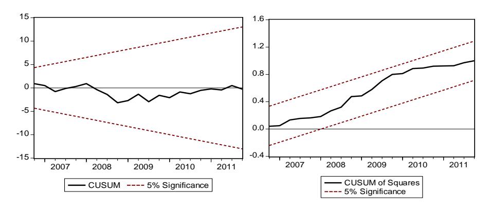
Fig. 1. Plots of the CUSUM and CUSUMSQ
3. Results
The findings in Table 2 indicate that all of the explanatory variables have significant influences on the Khanh Hoa domestic tourism demand in the short run and long run. The signs of the estimated coefficients seem to be in line with expectations, except for cost of living (CPI).
Table 2 Results of estimates of the domestic tourism demand in the long and short run.
| Variables | Symbol | Short-run elasticities | Prob. | VIF | Long-run elasticities |
|---|---|---|---|---|---|
| Domestic tourists | ΔLDT_1 | 0.266 | 0.0736 | 2.209 | |
| Temperature | \(\Delta AT_2\) | 0.197 | 0.0027 | 1.686 | .269 |
| Temperature | \(\Delta AT\_4\) | 0.138 | 0.0419 | 1.909 | .188 |
| Rainfall | \(\Delta RF\) | -0.001 | 0.0025 | 2.127 | 002 |
| Rainfall | \(\Delta RF_2\) | -0.001 | 0.0095 | 1.201 | 001 |
| Rainfall | \(\Delta RF\_4\) | -0.001 | 0.0966 | 2.350 | 001 |
| Sunshine hours | \(\Delta SH_2\) | 0.002 | 0.0628 | 2.065 | .003 |
| Vietnamese stock index | ΔLSI_1 | 0.359 | 0.0309 | 1.724 | .490 |
| Transport price index | ΔLTPI_1 | -12.571 | 0.0001 | 3.741 | -17.134 |
| Transport price index | ΔLTPI_3 | -3.831 | 0.0706 | 2.031 | -5.221 |
| Consumer price index | ΔLCPI_0 | -15.825 | 0.0034 | 2.159 | -21.569 |
| Consumer price index | ΔLCPI_1 | 9.466 | 0.0964 | 2.772 | 12.902 |
| Consumer price index | ΔLCPI_2 | 11.075 | 0.0198 | 1.676 | 15.095 |
| Consumer price index | ΔLCPI_3 | -21.933 | 0.0003 | 2.278 | -29.894 |
| Diagnostic tests | |||||
| R-squared | 0.807 | ||||
| Adjusted R-squared | 0.688 |
Effects Of Economic And Non-Economic Factors On Domestic Tourism Demand – A General-To-Specific Approach
| Normality test | 1.677 | 0.432 |
|---|---|---|
| Serial correlation LM test (2) | 0.282 | 0.757 |
| ARCH test (2) | 3.912 | 0.141 |
| White heteroskedasticity test | 32.52 | 0.254 |
| Ramsey RESET test (2) | 2.033 | 0.362 |
Note: LDT_1 means the log of domestic tourist has been taken first difference and lagged one quarter, analogously for other variables; VIF is variance inflation factor.
The coefficient of the lagged dependent variable reveals that habit persistence is one of the most important factors for explaining domestic tourism demand in Khanh Hoa. In total, 26.6% of domestic tourist arrivals to Khanh Hoa are affected by habit persistence or word-of-month. That is to say, there is a positively significant word-of-mouth effect on the domestic tourists' decision to select Khanh Hoa as a tourist destination. An increase in the demand for Vietnamese tourists is partly due to the positive influence of this factor. This result is also reasonable since a large number of visitors revisit Khanh Hoa.
As mentioned above, the weather variables were entered in the model including temperature, rainfall and sunshine. The coefficients and signs of these variables are significant and consistent with expectation. This implies that the demand for domestic tourism in Khanh Hoa is much dependent on the weather characteristics. In other words, the weather status may be one of the important factors in attracting domestic tourists to Khanh Hoa. In particular, the estimated coefficients of temperature and sunshine in the short run and long run suggest Vietnamese tourists are more likely to pick Khanh Hoa as a tourist destination as temperature and the number of sunshine hours increase. However, these effects are lagged from two to four quarters. Contrary to the impact of temperature and sunshine, the domestic tourist demand is affected by rainfall of current quarter and previous quarters both in the short run and the long run. The magnitude and sign of the elasticities indicate that greater rainfall would lead to a decline in the tourist arrivals to Khanh Hoa. These findings are in line with many previous studies such as Lyons, Mayor, and Tol, 2009 and Maddison (2001).
With regard to the influence of the stock index, the domestic tourist demand is also impacted positively by change in stock prices, as expected. On the other hand, because the magnitude of the coefficient is quite small (i.e. 0.002 in the short run and 0.003 in the long run), variances of securities prices on the security market have a small effect on tourism demand. The result of the estimation shows that a rise in stock index would imply an increase of the domestic tourist arrivals. However, its effect is lagged one quarter.
Contrary to the influence of the stock index, tourism costs have a very strong effect on domestic tourism demand, but the effect of living costs is ambiguous. Transportation costs have negative effects on the tourism demand in one to three previous quarters. The magnitude and sign of these coefficients suggest that when transportation costs increase, the domestic tourism demand drops substantially. Thus, tourism transportation suppliers should be careful with offering price policy in order to maintain the competitiveness of their transport services. Nevertheless, although the coefficients of CPI are significant, the signs of one and two quarters lag CPI are not as expected. One of the reasons explaining this problem is that in these quarters tourism costs in foreign countries are perhaps higher than those in Vietnam. Thus, though living costs for tourism inland can be high, Vietnamese tourists may still choose Khanh Hoa as a relevant tourist destination.
CONCLUSION AND POLICY IMPLICATION
In estimates of tourism demand, identifying the determinants as well as the employment of appropriate econometric models are of significance not only for academic researchers but also tourism practitioners (Song & Li, 2008). However, choosing the crucial influencing factors is in fact dependent on the availability of data and their economic significance. In this study, both economic and non-economic variables were included in the model. The variables used for measurement of weather change in Khanh Hoa are temperature, sunshine, and rainfall, while the Vietnamese stock index, the Vietnamese transportation price index and the Vietnamese consumer price index are considered as the proxies of economic variables. In addition, the habit persistence of tourists is also considered as an explanatory variable of domestic tourism demand. On the other hand, the single equation in a semi-log linear functional form is applied for estimating domestic tourism demand in Khanh Hoa. Among different tourism demand modelling approaches, the general-to-specific approach stated with a general dynamic model is found to be the most appropriate.
The study concludes that the domestic tourism demand is affected by temperature, rainfall and sunshine in Khanh Hoa, the stock index, the transportation price and the consumer price in Vietnam. However, the effects of these variables on the behaviour of Vietnamese tourists' destination of choice are different in both the long run and short run. The positively lagged dependent variable suggests that word-of-mouth recommendation to potential tourists provides good signs in terms of Khanh Hoa's tourism industry. It implies that past visits have certain positive effects on the decision-making process for present demand. This positive image with tourism service quality, natural environment and others should, therefore, be maintained and developed through tourism promotion activities. Tourism suppliers should resume improving their service quality, and/or provide tourism products and services with a variety of highly desirable characteristics to increase competition. In addition, the weather factors are important influencing factors in the holiday decision-making process of tourists. Tourism operators should thus provide weather and climate information in their tourism brochures to Vietnamese tourists. On the other hand, the movement of stock prices on the securities market has certain positive influence on tourism demand. A growing securities market will be a constructive sign for development of a domestic tourism market in the long term.
Moreover, the results indicated that sensitiveness of domestic tourist demand due to change in tourism costs is very high. Thus, to attract more Vietnamese tourists to Khanh Hoa, tourism operators should have affordable prices with regard to both products and services, and design many different attractively priced holiday packages as well as offer special financial treatment such as discounts or bonuses for loyal tourists.
Appendixes
Appendix I. Results of regressions and tests for the relationship between the stock and the GDP
Table I.1 Test of stationarity of GDP and Stock Index (SI).
| Level | First difference | |||
|---|---|---|---|---|
| Variables | Coefficient | Prob. | Coefficient | Prob. |
| 1. Exogenous: Constant, Linear Trend | ||||
| GDP | 0.9843 | 0.9986 | -3.9647* | 0.0795 |
| SI | -1.6661 | 0.6823 | -2.6113 | 0.2961 |
| 2. Exogenous: Constant | ||||
| GDP | 4.6454 | 1.0000 | -0.1022 | 0.9164 |
| SI | -1.9540 | 0.2976 | -2.8732* | 0.0907 |
Note: SI is the Vietnamese stock index; GDP is the Vietnamese GDP; * is a 10% significance level.
Table I.2 Result of regression and diagnostic tests.
| Variable | Coefficient | Prob. |
|---|---|---|
| Constant | 556.18 | 0.0096 |
| GDP | -0.0009 | 0.0418 |
| TREND | 217.15 | 0.0264 |
| Diagnostic tests | ||
| R-squared | 0.5476 | |
| Adjusted R-squared | 0.4183 | |
| Durbin-Watson stat | 1.8893 | |
| F-statistic | 4.2357 | 0.0623 |
| Jarque-Bera test | 0.7496 | 0.6874 |
| Serial correlation LM test | 3.6164 | 0.1640 |
| ARCH (1) test | 2.1969 | 0.1383 |
| White heteroskedasticity test | 4.3322 | 0.3629 |
| Ramsey RESET(1) test | 3.3800 | 0.0660 |
Note: Dependent variable is SI, and TREND is the time trend.
Vo Van Can
Table I.3 Test of cointegration of residual.
| t-Statistic | Prob. | ||
|---|---|---|---|
| Augmented Dickey-Fuller test statistic | -3.13849 | 0.0637 | |
| Test critical values: | 1% level | -4.58265 | |
| 5% level | -3.32097 | ||
| 10% level | -2.80138 |
Appendix II. Results of looking for optimal weather factors
Model expressing relationship between the domestic tourists and the weather variables:
\[LDT = \lambda_0 + \lambda_1 F_i + \lambda_2 F_i^2\] where LDT is the log of the domestic tourists; λ0, λ1, and λ2 are coefficients to be estimated; F is weather factor; and i is temperature, rainfall, or sunshine.
Including both linear and quadratic variables in the models implies that there are optimal weather factors for tourism (Lise & Tol, 2002). According to Lise and Tol (2002), the optimal weather factors ( can be calculated by formula: and its standard deviation (σopt) is approximated with its first-order Taylor expansion:
\[\sigma_{opt}^2 \approx \frac{1}{4\lambda_2^2} \sigma_{\lambda_1}^2 + \frac{\lambda_1^2}{4\lambda_2^4} \sigma_{\lambda_2}^2 - \frac{\lambda_1}{2\lambda_2^3} \sigma_{\lambda_1} \sigma_{\lambda_2}\]
Table II shows the results of regressions and the optimal weather factors as well as their t-statistic.
Table II. Results of regression and optimal weather factors.
| Variable | Coefficients | t-statistic |
|---|---|---|
| Constant | -18.951 | 70.512 |
| Temperature | 2.246 | .387 |
| Squared temperature | 040 | 263 |
| Optimal temperature | 27.874 | 17.870 |
| Constant | 12.143874 | 70.512 |
| Rainfall | .000768 | .387 |
| Squared rainfall | .000001 | 263 |
| Optimal rainfall | 444.137 | .630 |
| Constant | 14.02773 | 11.536 |
| Sunshine | 02048 | -1.590 |
| Squared sunshine | .00005 | 1.627 |
| Optimal sunshine | 191.463 | 10.951 |