

1. INTRODUCTION
Optimum food utilization strategy is one of the important efforts to increase meat production of livestock. The dynamics of livestock growth over time is needed to obtain an optimal growth strategy of animal feeds. Mathematical models of the growth curve could be used to determine the selection of suitable feeding materials for livestock development [1]. In addition, the growth curve could also be used to determine the age of livestock slaughter to be optimal. Moreover, the growth curve model could be used as a parameter in pre-harvest methods in large livestock such as cattle, buffalo, goats, and sheep. The mathematical model of livestock growth could also be used to analyze the efficiency of livestock production over the lifetime (lifetime production efficiency) [2].
The growth process of livestock, including poultry, could be measured from mass (weight) profile of the livestock versus time [3], [4]. Livestock and poultry growth generally follows a sigmoidal pattern. Poultry growth usually starts with an accelerating growth phase from hatching. Then, poultry attains the maximum growth rate at a certain time (the inflection time). After that, poultry growth is decelerating. At final phase, poultry weight generally tends to a limiting value (asymptote) mature weight [1], [5].
Many nonlinear growth curves have proposed to describe and fit the sigmoid relationship between poultry weight and time. Logistic model, Gompertz model. and Richards model are commonly for describing a relationship between poultry weight and time [1], [3], [5]. Richards and Gompertz models gave good descriptions of weight growth in many animal species including chicken, cattle, elks, ostrich, turkey, and emus. Gompertz growth model has applied as the growth model for chicken. Gompertz model fitted many actual data and its parameters had biological interpretations [6], [7], [8]. Moreover, the Gompertz model has good fitting for weight information whose inflection points occur, when approximately 35 - 40% of growth have been achieved [5].
Accurate and straightforward growth models are useful for describing life individual growth. In this paper, we present a new mathematical model for the growth function of a living organism. The model was derived from the modified logistic differential equation. Then, the model was implemented to describe body weight growth of chicken (rooster and hen), where the growth data cite from literature. The accuracy of predicted results from the model was compared to the standard logistic model, Gompertz model and Richards model.
This paper is organized as follows. Section 2 presents some modified logistic growth models. The proposed model and its main property is discussed in section 3. Implementations of the proposed model, logistic model,
Received April 23th, 2018, Revised July 17th, 2018 (first) and November 12th, 2018 (second), Accepted for publication December 20th, 2018. Copyright ©2018 Published by Bio Mathematical Society, e-ISSN: 2549-2896, DOI:10.5614/cbms.2018.1.2.5
Gompertz model and Richard model on chicken (rooster and hen) data cited from the literature are presented in Section 4. Conclusions are written in the last section.
2. MODIFIED LOGISTIC GROWTH MODEL
The first mathematical model describing population growth is the Malthus model or exponential model [9]. Let y(t) is population size at time t In the exponential model, the growth rate \(\frac{dy}{dt}\) is assumed proportional the size of existing population y(t). The exponential model could be represented by the following differential equation
\[y(t) = Y_0 \exp(rt). \tag{1}\]
Here r is the proportional growth rate parameter. The exponential growth model in Eq. (1) is rarely used to describe population growth, since it produces an unbounded population growth.
The exponential growth model was improved by logistic growth model. In the logistic model, a population grows until it attains a maximum capacity [9]. The logistic model is based on the assumption that the growth rate \(\frac{dy}{dt}\) is proportional to the existing population and the remaining resources available to the existing population. The logistic growth model be expressed as
\[y(t) = \frac{K}{1 + \exp(-rt)\left(\frac{K}{Y_0} - 1\right)} = \frac{K}{1 + \exp[-r(t - t_{\inf})]},\] (2)
where
\[t_{\rm inf} = -\frac{1}{r} \ln \left( \frac{K}{Y_0} - 1 \right). \tag{3}\]
When y(t) represents body weight of a livestock at time t, then parameter K in Eq. (2) could be considered as the mature weight (the maximum weight that could be attained by livestock). Here \(t_{\inf}\) is the inflection time (the optimal time of a population growth).
The logistic growth model has various modifications. One of the modified version is the shifted logistic function. The first version of the shifted logistic function could be presented in the following form [10]
\[y(t) = K \left( \frac{1}{1 + \exp(-r(t - t_{\text{inf}}))} - \frac{1}{1 + \exp(rt_{\text{inf}})} \right).\] (4)
The second version and the third version of the shifted logistic function could be expressed as [11]
\[y(t) = \frac{K}{1 + \exp(-r(t - t_{\text{inf}}))} + L\] (5)
and
\[y(t) = \frac{K + Mt}{1 + \exp(-r(t - t_{\text{inf}}))} + L\] (6)
respectively. Here, L and M are additional parameters.
Modification of the logistic growth model also occurred in the differential equations model. The logistic differential equation has been modified into von Bertalanffy, Richards, Gompertz, Blumberg, Turner et al. and Tsoularis differential equations. The von Bertalanffy differential equation has the following form [12], [13]
\[\frac{dy}{dt} = ry^{\frac{2}{3}} \left( 1 - \left( \frac{y}{K} \right)^{\frac{1}{3}} \right), \ y(0) = Y_0.\] (7)
Richards (1959) proposed a modified logistic differential equation so-called Richards differential equation. The Richards differential equation has the following form [13], [14]
\[\frac{dy}{dt} = ry\left(1 - \left(\frac{y}{K}\right)^{\beta}\right), \ y(0) = Y_0. \tag{8}\]
Gompertz differential equation is a limiting case of a modified logistic differential equation. The Gompertz differential equation is derived from
\[\frac{dy}{dt} = \lim_{\beta \to 0} \frac{ry\left(1 - \left(\frac{y}{K}\right)^{\beta}\right)}{\beta} = ry\ln\left(\frac{K}{y}\right), \ y(0) = Y_0. \tag{9}\]
Blumberg (1968) also introduced a modification of logistic differential equation so called the hyper logistic function, accordingly [13], [15]
\[\frac{dy}{dt} = ry^{\alpha} \left( 1 - \frac{y}{K} \right)^{\gamma}, \ y(0) = Y_0. \tag{10}\]
Turner et al. (1976) proposed a modified logistic differential equation which they named the generic growth function. The modification has the following form [13], [16]
\[\frac{dy}{dt} = ry^{1+\beta(1-\gamma)} \left(1 - \left(\frac{y}{K}\right)^{\beta}\right)^{\gamma}, \ y(0) = Y_0. \tag{11}\]
Tsoularis (2001) proposed a more general modification of logistic differential equation. The Tsoularis differential equation has the form [13]
\[\frac{dy}{dt} = ry^{\alpha} \left( 1 - \left( \frac{y}{K} \right)^{\beta} \right)^{\gamma}, \ y(0) = Y_0.\] (12)
In the next section, we propose another version of a modified logistic differential equation.
3. THE PROPOSED MODEL
The logistic growth model and the modified logistic growth model presented in the previous section could be represented in the Kolmogorov form
\[\frac{dy}{dt} = yP(y) \tag{13}\] for some continuous function P. For classical (standard) logistic differential equation, the function P is \(P(y) = r(1 - \frac{y}{K})\). In the logistic growth model, it is assumed that the growth rate of a population is proportional to the population number at the current time. Here, we modify the model in Eq. (13) in more general form, namely
\[\frac{dy}{dt} = F(y) \tag{14}\] for some continuous function F. A simple growth model satisfies Eq. (14) but it does not satisfy the Kolmogorov form in Eq. (13), is the monomolecular model. The monomolecular model satisfy the following differential equation [17]
\[\frac{dy}{dt} = q - sy, y(0) = Y_0. \tag{15}\]
Here, q could be considered as constant growth rate while s could be considered as the death rate of a population.
In this section, we propose a generalized model of the monomolecular model and the standard logistic growth model. We extend the monomolecular model and the logistic differential equation model into the following differential equation.
\[\frac{dy}{dt} = (q + ry)\left(1 - \frac{y}{K}\right), \quad y > 0 \tag{16}\] and the initial condition \(y(0) = Y_0 > 0\). Note that region of biological interest of the model in Eq. (16) is \(\mathbf{R}_+ := \{x \in \mathbf{R} : x > 0\}\), since a life organism could not grow from nothing. Here, q and r could be considered as constant growth rate and proportional growth rate respectively.
The modified logistic growth model in Eq. (16) has one equilibrium, namely y = K. Global stability of the equilibrium is presented in the following theorem.
Theorem 3.1. The equilibrium y = K is globally asymptotically stable.
Proof: We define a Lyapunov function \(V: \mathbf{R} \to \mathbf{R}\) by \(V(y) = (y - K)^2\). The function V is a \(C^{\infty}(\mathbf{R})\) function. In addition, the equilibrium y = K is the global minimum of V. Moreover, V is a definite positive function around the equilibrium where every \(y \in R \setminus \{K\}, V(y) > 0\). The time derivative of V computed along solutions of the mathematical model in Eq. (16) is given by the expression
\[\frac{dV}{dt} = \frac{-2}{K} (q + ry) (y - K)^{2}.\]
Since all parameters in the model are positive and the variable y is positive, it follows that \(\frac{dV}{dt} \le 0\) for y > 0. In addition \(\frac{dV}{dt} = 0\) if and only if y = K. Therefore the greatest compact invariant set in \(\left\{y \in \mathbf{R}_+ : \frac{dV}{dt} = 0\right\}\) is the singleton \(\{K\}\). By LaSalle's invariance principle [18], the equilibrium y = K is globally asymptotically stable in \(\mathbf{R}_+\).
The population weight at the inflection time (\(t_{\rm inf}\)) could be determined as follows. By differentiating both sides of Eq. (16) and setting \(\frac{d^2y}{dt^2}(t_{\rm inf})=0\), we find
\[y\left(t_{\rm inf}\right) = \frac{K}{2} - \frac{q}{2r}.\tag{17}\]
Hence, the population weight at the inflection time for this model is smaller than the values obtained from the logistic growth model. Exact values of the inflection time could be obtained whenever the analytical solution of the model in Eq. (16) could be found.
The differential equation in Eq. (16) could be written as
\[\left(\frac{r}{q+ry} + \frac{1}{K-y}\right)dy = \left(\frac{q}{K} + r\right)dt.\]
By integrating the left side with respect to y and the right side with respect to t gives
\[\ln\left(\frac{q+ry}{K-y}\right) = \left(\frac{q}{K}+r\right)t + c_0\tag{18}\] for some constant \(c_0\). The mathematical expression in the Eq. (18) could be written as
\[\frac{q+ry}{K-y} = c_1 \exp\left(\left(\frac{q}{K} + r\right)t\right), c_1 = \exp\left(c_0\right). \tag{19}\]
By solving Eq. (19) for y, it could be obtained explicit solution of the modified logistic differential equation as
\[y(t) = \frac{c_1 K \exp\left(\frac{qt}{K} + rt\right) - q}{r + c_1 \exp\left(\frac{qt}{K} + rt\right)}.\] (20)
By substituting the initial condition \(y(0) = Y_0\), then \(c_1 = \frac{qY_0 + a}{K - Y_0}\). Hence, the explicit solution in Eq. (20) could be written as
\[y(t) = \frac{K - q\left(\frac{K - Y_0}{rY_0 + q}\right) \exp\left(\frac{-qt}{K} - rt\right)}{1 + r\left(\frac{K - Y_0}{rY_0 + q}\right) \exp\left(\frac{-qt}{K} - rt\right)}.\] (21)
By defining the following parameters
\[\alpha = \frac{q}{K} + r, \quad A = K - q \left( \frac{K - Y_0}{r Y_0 + q} \right), \quad B = r \left( \frac{K - Y_0}{r Y_0 + q} \right), \tag{22}\] then the modified logistic growth model in Eq. (21) could be written as
\[y(t) = \frac{K - (K - A)\exp(-\alpha t)}{1 + B\exp(-\alpha t)}.\] (23)
Here \(\alpha, A, B, K\) are positive parameters and \(A \le K\). The parameter \(\alpha\) is effective growth rate, K is the maximum capacity (mature weight), while the parameter A, B are corresponding to initial weight and inflection time. The inflection time ( \(t_{inf}\)) of the model in Eq. (23) is
\[t_{\inf} = \frac{\ln B}{\alpha} = \frac{K}{q + rK} \ln \left( r \left( \frac{K - Y_0}{rY_0 + q} \right) \right). \tag{24}\]
The inflection time in (24) could be determined by evaluating the second derivative of y in Eq. (23) and setting \(\frac{d^2y}{dt^2}(t_{\rm inf})=0\). If the constant growth rate parameter (q) is zero, then the inflection time in Eq. (24) could be simplified into Eq. (3). From Eq. (24), the modified logistic growth model in Eq. (23) could be presented in the following form
\[y(t) = \frac{K - (K - A)\exp(-\alpha t)}{1 + \exp(-\alpha(t - t_{\inf}))}.\] (25)
Since there are some well-known modified logistic growth model, then the presented growth model presented in Eq. (29) could be called by a WEP-modified logistic growth model. Here WEP comes from Windarto-Eridani-Purwati.
4. EXTENSION OF THE PROPOSED MODEL
It is well known that the length and weight of fish species will grow until they attain some maximum values. By applying the presented model in the previous section, the dynamics of fish weight and fish length could be modeled by following differential equations
\[\frac{dW}{dt} = (q_w + r_w W) \left( 1 - \frac{W}{K_w} \right), \quad W(0) = w_0,\] (26)
and
\[\frac{dL}{dt} = (q_l + r_l L) \left( 1 - \frac{L}{K_l} \right), \quad L(0) = l_0, \tag{27}\]
respectively. Here, W(t) and L(t) are fish weight and fish length at time t respectively. In Eq. (26)-(27), \(q_w\), \(q_l\) are constant growth rate of fish weight and fish length, while \(r_w\), \(r_l\) are proportional growth rate of fish weight and fish length respectively. By applying the analytical solution of the previous section, we found dynamic of fish weight and fish length could be described by
\[W(t) = \frac{K_w - q_w \left(\frac{K_w - w_0}{r_w w_0 + q_w}\right) \exp\left(\frac{-q_w t}{K_w} - r_w t\right)}{1 + r_w \left(\frac{K_w - w_0}{r_w Y_0 + q_w}\right) \exp\left(\frac{-q_w t}{K_w} - r_w t\right)}\](28)
and
\[L(t) = \frac{K_l - q_l \left(\frac{K_l - l_0}{r_l l_0 + q_l}\right) \exp\left(\frac{-q_l t}{K_l} - r_l t\right)}{1 + r_l \left(\frac{K_l - l_0}{r_l l_0 + q_l}\right) \exp\left(\frac{-q_l t}{K_l} - r_l t\right)}\](29)
respectively.
It is also well known that there is length-weight relationship (LWR) of fish species. A mathematical equation was used to show relationships between the average weight of fish at a given length [19], [20]. The length-weight relationship is given by
\[W(t) = aL(t)^b. (30)\]
Here a and b are empirical parameters. Typically, the b parameters range from 2 to 4. Fish can attain either isometric or allometric growth. Isometric growth indicates that both fish length and fish weight are increasing at the same rate [20]. Here, we estimated parameters empirical parameters a and b for the threadfin bream (Nemipterus marginatus) from the South China Sea, where the data cited from literature [21]. The length-weight relationship data is shown in Table I.
TABLE I: Length-weight relationship data for the threadfin bream (Nemipterus marginatus)
| L (cm) | W (grams) | L (cm) | W (grams) |
|---|---|---|---|
| 8.1 | 6.3 | 16.6 | 65.6 |
| 9.1 | 9.60 | 17.7 | 69.4 |
| 10.2 | 11.6 | 18.7 | 76.4 |
| 11.9 | 18.5 | 19 | 82.5 |
| 12.2 | 26.2 | 20.6 | 106.6 |
| 13.8 | 36.1 | 21.9 | 119.8 |
| 14.8 | 40.1 | 22.9 | 169.2 |
| 15.7 | 47.3 | 23.5 | 173.3 |
By taking natural logarithm of eq. (30), the relationship could be converted into
\[ln W = ln a + b ln L.\] (31)
Then by using linear regression method, we find the parameter values of \(\ln a = -4.53786\) and b = 3.05735. Hence the parameter value of a is 0.01070. Since the parameter value of b does not significantly differ from 3, then the species attain isometric growth [20]. In order to estimate parameters in Eq. (28) and (29), we need fish weight and fish length data over time. In the next section, we apply the proposed model (WEP-modified logistic growth model) to some secondary data cited from the literature.
5. APPLICATION OF THE PROPOSED MODEL
In this section, the proposed model is implemented to describe chicken body weight (rooster and hen) growth, where the data are cited form literature [3], [22]. Rooster (x) and hen (y) body weight at different age (t) are presented in Table 2. In addition, accuracy result of the proposed model will be compared to the logistic model, Gompertz model, and Richards model. The logistic model was presented in Eq. (2), while Richards and Gompertz differential equations were presented in Eq. (8) and (9) respectively. Analytical solution of the Richards differential equation in Eq. (8) was given by
\[y_R(t) = \frac{K}{\left[1 + \beta \exp(-r\beta(t - t_{\text{inf}}))\right]^{\frac{1}{\beta}}},\] (32)
where the inflection time \(t_{\inf} = \frac{1}{r\beta} \ln \left( \frac{(\frac{K}{Y_0})^{\beta} - 1}{\beta} \right)\). By defining \(m = \beta + 1, \ r^* = r\beta\), then the Richards growth model in Eq. (32) could be expressed as
\[y_R = K \left[ 1 - (1 - m) \exp\left( -r^*(t - t_{\text{inf}}) \right) \right]^{\frac{1}{(1 - m)}}.\] (33)
Exact solution of the Gompertz differential equation in Eq. (9) was given by
\[y_G(t) = \frac{K}{\exp(\exp(-r(t - t_{\text{inf}})))}\] (34)
where \(t_{\inf} = \frac{1}{r} \ln \left( \ln(\frac{K}{Y_0}) \right)\). Some authors used the following Gompertz-Laid growth model [3]
\[y_G(t) = W_0 \exp\left(\exp(rt_{\text{inf}}) \left(1 - \exp(-rt)\right)\right). \tag{35}\]
Here, \(W_0\) is initial chicken weight in the Gompertz model and m is the shape parameter in Richards model. For m=2, then the Richards model could be simplified into logistic model. For m tends to one, then the Richards model could be simplified into the Gompertz model.
| t (days) | x (grams) | y(grams) | t (days) | x (grams) | y (grams) |
|---|---|---|---|---|---|
| 0 | 37 | 36.68 | 42 | 519.72 | 436.51 |
| 3 | 41.74 | 40.8 | 45 | 577.27 | 480.31 |
| 6 | 59.19 | 57.33 | 48 | 633.59 | 522.91 |
| 9 | 79.94 | 77.24 | 51 | 667.18 | 547.23 |
| 12 | 102.96 | 97.96 | 54 | 717.17 | 583.56 |
| 15 | 132.13 | 121.92 | 57 | 786.35 | 631.77 |
| 18 | 170.18 | 155.08 | 71 | 1069.28 | 832.57 |
| 21 | 206.56 | 184.24 | 85 | 1326.49 | 1009.48 |
| 24 | 250.71 | 218.37 | 99 | 1589.71 | 1183.8 |
| 27 | 285.27 | 247.12 | 113 | 1859.26 | 1440.18 |
| 30 | 324.92 | 279.58 | 127 | 2015.44 | 1561.89 |
| 33 | 372.83 | 319.55 | 141 | 2142.31 | 1619.34 |
| 36 | 417.41 | 355.13 | 155 | 2220.54 | 1680.29 |
| 39 | 469 13 | 396.32 | 170 | 2262 63 | 1717 78 |
TABLE II: Means of rooster and hen chicken weight data
There are four parameters in the model should be estimated, namely parameter \(\alpha\) (effective growth rate), K (maximum weight/ mature weight of chicken), the inflection time \(t_{inf}\) and parameter A (correspond to the initial chicken weight). Since growth function of the model is explicitly presented in the Eq. (25), then nonlinear regression procedures could be applied to estimate the parameters.
The parameters \(\alpha\), K, \(t_{inf}\) and A are estimated such that the normalized residual sum of squares (NRSS)
\[NRSS = \sum_{i} \frac{(z_i - \hat{z}_i)^2}{(z_i - \overline{z})^2}, z = x \lor z = y\] (36)
is minimum. In Eq. (36), \(\bar{z}\) is the average of z and \(\hat{z}_i\) is chicken weight at time i predicted from the model. The normalized residual sum of square corresponds to the determination coefficient via the following relation
\[R^2 = 1 - NRSS. (37)\]
Parameters in the logistics, Gompertz, and Richards model also be estimated with a similar manner. The accuracy of the predicted results could also be measured by evaluation of Mean Absolute Percentage Error (MAPE), which is given by the following formula
\[MAPE = \sum_{i} \frac{1}{n} \left| \frac{z_i - \hat{z_i}}{z_i} \right| 100\%. \tag{38}\]
Here n is the number of observational data. The nonlinear least square (nls) procedure of R open source software is used to estimate parameters of the proposed model, logistic, Gompertz, and Richards model. R open source software was built by the R Foundation for Statistical Computing. Estimation results of the proposed model, logistic, Gompertz, and Richards model for rooster and hen weight, the determination coefficient \((R^2)\) and Mean Absolute Percentage Error (MAPE) for the models are presented in Table III, while the dynamics of rooster weight and hen weight are shown in Fig. 1 and Fig. 2 respectively.
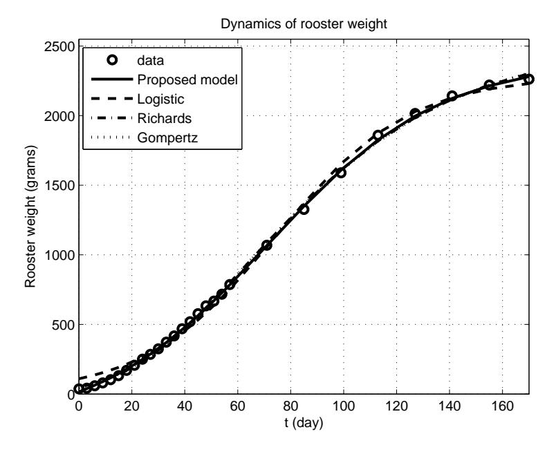
Fig. 1: Dynamic of rooster weight.
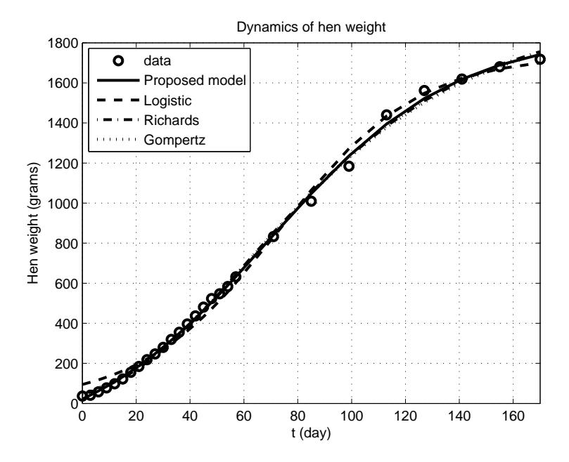
Fig. 2: Dynamic of hen weight.
TABLE III: Estimated parameters for the proposed model, logistic, Richards and Gompertz growth model
| Model | Parameters | Rooster | Hen |
|---|---|---|---|
| The proposed model | Mature weight (K) | 2399.749 | 1847.162 |
| (WEP-modified logistic | Effective growth rate (α) | 0.031 | 0.029 |
| growth model) | Inflection time (tinf ) | 71.584 | 69.015 |
| A | 166.323 | 183.061 | |
| NRSS | 0.00031 | 0.00119 | |
| 2 R | 0.99969 | 0.99881 | |
| MAPE | 0.04754 | 0.04267 | |
| Logistic model | Mature weight (K) | 2279.904 | 1739.652 |
| Growth rate (r) | 0.040 | 0.039 | |
| Inflection time (tinf ) | 74.677 | 73.331 | |
| NRSS | 0.00357 | 0.00501 | |
| 2 R | 0.99643 | 0.99499 | |
| MAPE | 0.299927 | 0.25398 | |
| Richards model | Mature weight (K) | 2512.972 | 1945.342 |
| Growth rate (r*) | 0.023 | 0.021 | |
| Inflection time (tinf ) | 64.307 | 61.344 | |
| Shape parameter (m) | 1.054 | 0.978 | |
| NRSS | 0.00071 | 0.00175 | |
| 2 R | 0.99929 | 0.99825 | |
| MAPE | 0.07373 | 0.06552 | |
| Gompertz model | Growth rate (r) | 0.022 | 0.021 |
| Inflection time (tinf ) | 63.498 | 61.704 | |
| Mature weight (K) | 2539.651 | 1936.385 | |
| NRSS | 0.00073 | 0.00175 | |
| 2 R | 0.99927 | 0.99825 | |
| MAPE | 0.06007 | 0.07031 |
It could be seen from Fig. 1 and Fig. 2 that rooster growth and hen growth follow sigmoidal patterns. Rooster growth and hen growth stars by an accelerating growth phase from hatching. Then, the chicken attains a maximum growth rate at the inflection time. At final phase, the chicken weight tends to a mature weight. Qualitatively, all of the models, describe the chicken growth well, as seen in the figures. But, if we compare its MAPE, as seen in Table III, we see that the logistic model have the biggest MAPE, and it mean that its accuracy is poorer than the other models. This apparently due to the logistic model is not accurate in predicting the dynamics of rooster and hen weight at the early times (Fig. 1 and Fig. 2). By adding one additional parameter (q) to the presented model, the dynamics of rooster and hen weight could be better estimated by using the presented model.
From the Table III, it was found that the growth rate (the effective growth rate) or the maturation rate (α in the proposed model, r in the logistic and Gompertz model and r ∗ in the Richards model) was higher in rooster than in hen. This result is consistent with the result from Aggrey (2002) [3]. It also could be found that inflection time of the proposed model is relatively close to inflection time of the logistic model. In addition, inflection time of the Richards model is relatively close to the Gompertz model. It is apparently due to the shape parameter m in the Richards model is close to one. Moreover, it was found that the proposed model, logistic model, Richards model, and Gompertz model produced a high determination coefficient (R2 is greater than 0.99). Although the determination coefficients of the four models did not differ significantly, Mean Absolute Percentage Error (MAPE) of the models considerably varied. It was found the proposed model has the smallest MAPE, which is 4.754% in rooster and 4.267% in hen. This indicates that the proposed model could be used as an alternative model to describe poultry growth curve or individual growth.
6. CONCLUSION
A new growth model was presented in this paper. The model was derived from the modification of logistic differential equation. The proposed model also was simulated and verified using rooster and hen weight data cited from the literature. The estimation results from the model ware compared to the logistic model, Richards, and Gompertz growth model. It was found that the model gave better results compared to the logistic model, Richards, and Gompertz growth model. It indicates that model could be used as an alternative model to describe poultry growth curve or individual growth.
ACKNOWLEDGEMENT
Part of this research was funded by General Directorate of Higher Education (Ditjen DIKTI), Ministry of Research, Technology and Higher Education Republic Indonesia through "Penelitian Unggulan Perguruan Tinggi (PUPT)" project.
CONFLICT OF INTEREST
The authors do not have conflict of interest in regard to this research or its funding.