

1. Introduction
Mathematical models, which are deterministic or stochastic, have been widely used to understand complex phenomena [22], [20], [21], [24]. In general, the deterministic mathematical models are used because it easier to handle [29], [10]. The model is in the form of a system of linear or nonlinear differential equations. Although some analytical calculation such as equilibrium points or stability can be made, the analytical solution of the model is not easily derived. Therefore, a numerical approach is generally used.
A number of numerical methods have been developed and widely used to solve mathematical models [6]. Of these, Runge-Kutta method is one of the well-established numerical technique that has been widely implemented. This scheme is a foundation for the development of MATLAB ode45 routine, which is mostly used to solve differential equations [30]. This routine is generally stable and can generate the properties and behavior of the models such as chaotic and oscillation [30], [14]. Therefore, this has been extensively used to solve many deterministic mathematical models [14], [22], [32]. There are also other alternative numerical techniques that can be used when the well-established numerical methods fail in generating the solutions. They are the Differential Transformation Method (DTM for short) [34], [8] and the Non Standard Finite Difference Scheme (NSFDS for short) [15], [16], [3]. These are the promising approach used to solve deterministic mathematical models.
The DTM is a semi-analytic numerical technique which depends on the Taylor series. This method was first proposed by Zhou [34] and has been modified to overcome its limitation [26], [25]. The DTM gives an analytical solution in the form of a polynomial and does not require symbolic computation of the derivatives. This method has been applied for solving various problems [26], [23], [4]. However, the classical DTM has some drawbacks: the obtained solution may diverge from the exact solution and gives good approximation only in a small region. Therefore, to overcome and improve its accuracy, it is required to divide the time domain into n sub-domain [26], and hence the system of equations can be solved in each domain. Different to Runge-Kutta, this scheme is implemented directly to the model without requiring linearisation or discretisation [4], [26]. This may avoid the error due to discretisation [26]. The NSFDS is another numerical scheme that has been proposed by Mickens [15]. This scheme is based on the standard finite difference scheme but the denominator part is substituted by a nonnegative function \(\phi(h)\) and a nonlocal approximation of nonlinear terms is used [15], [17]. Different from the DTM, the scheme is constructed by discretising the equation.
The DTM and NSFDS have been utilised to solve many deterministic mathematical models. In general, the solutions of both approaches can generate the model's behaviour such as oscillations and chaos [27],
[31], [26]. Motivated by this, in this paper, we employ the DTM and NSFDS for solving a plant disease mathematical model. Since analytical solutions of the model cannot be generated, we cannot compare their numerical solutions to the exact ones. However, because the well-established MATLAB ode45 routine, which is based on Runge-Kutta method, can provide the solutions of the model, we compare the numerical solutions using the DTM and NSFDS to that of the MATLAB ode45 routine. This aims to determine the performance of the DTM and NSFDS.
This paper is organised as follows. Section 2 presents the numerical methods. In Section 3, mathematical model of plant disease transmission is presented. In Section 4, the DTM and NSFDS for the model is presented followed by the numerical experiments in the next section. Finally, the discussions and conclusions are presented.
2. NUMERICAL METHODS
This section presents the differential transformation method (DTM) and nonstandard finite difference scheme (NSFDS). These methods are used to solve plant disease mathematical models and then the numerical results of them are compared.
2.1. Differential Transformation Method
The DTM is a semi analytical numerical approach that depends on the Taylor series. The method can be used for solving linear and non-linear differential equations. It uses the form of polynomial as approximations of the solutions [12], [26], [4], [25], [8]. Here we employ the DTM to solve a plant disease mathematical model.
With reference to the articles [26], [25], [8], [4], the basic definitions of the differential transformation are given as follows.
Definition 1. Let f(x) is a differentiable function then the differential transform of k th derivative of that function is defined as
\[F(k) = \frac{1}{k!} \left[ \frac{d^k f(x)}{dt^k} \right] \tag{1}\] where f(x) is the original function and F(x) is the transformed function.
Definition 2. The differential inverse of the transformed function is defined as
\[f(x) = \sum_{k=0}^{\infty} F(k)(x - x_0)^k.\] (2)
From Equation (1) and (2), we obtain
\[f(x) = \sum_{k=0}^{\infty} \frac{(x - x_0)^k}{k!} \frac{d^k f(x)}{dx^k} |_{x = x_0}.\] (3)
Equation (3) means that the concept of DTM is obtained from Taylor series expansion.
Using definitions (1) and (2), we can obtain the operation properties of the DTM as presented in Table I. In real application, we only use finite series for f(x) as
\[f(x) = \sum_{k=0}^{n} F(k)(x - x_0)^k.\] (4)
This is known as the classical differential transformation method. In this paper, we employ multi-step differential transformation method [26], which is explained below.
Suppose that we aim to derive the solution in the time domain (0, X). The time domain is divided into m subintervals [xm−1, xm] (see Figure 1). For the first time domain, [0, x1], the solution is approximated using
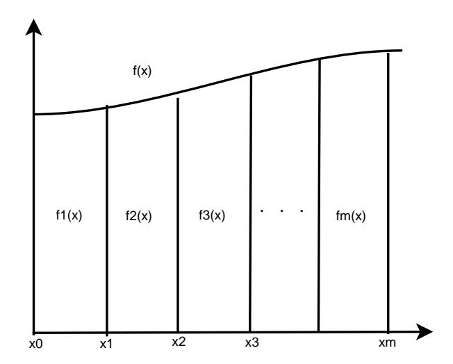
Fig. 1: Time step and approximation function in each domain
\[f_1(x) = \sum_{k=0}^{n} F_1(k) x^k.\] (5)
with initial condition \(f_1(0) = f_0\). For \(m \ge 2\), and at each subintervals \([x_{m-1}, x_m]\), the initial conditions is the value of f(x) at the last time of the previous time step, \(f_{m-1}(m-1) = f_m(0)\) and is approximated using
\[f_m(x) = \sum_{k=0}^n F_m(k)(x - x_{m-1})^k, \quad x \in (x_{m-1}, x_m).\] (6)
The solution is given by
\[f(x) = \begin{cases} f_1(x), & t \in (0, x_1), \\ f_2(x), & t \in (x_1, x_2) \\ \vdots \\ f_m(x), & t \in (x_{m-1}, x_m). \end{cases}\] (7)
Let u(t) and v(t) are two functions with time t and U(z) and V(z) are transformed functions corresponding to u(t) and v(t), the operations of differential transformation are given in Table I.
TABLE I: Operation of differential transformation
| Original function | Transformed function |
|---|---|
| f(t) = u(t) + v(t) | F(z) = U(z) + V(z) |
| f(t) = au(t) | F(z) = aU(z) |
| f(t) = u(t)v(t) | \(F(z) = \sum_{l=0}^{k} V(l)U(z-1)\) |
| \[f(t) = \frac{d^m u(t)}{dt^m}\] | \[F(z) = (z+1)(z+2)(z+3)\dots(z+m)U(z+m)\] |
| \[f(t) = \frac{d\vec{u}(t)}{dt}\] | F(z) = (z+1)F(k+1) |
| \(f(t) = t^{m^2}\) | \(F(z) = \delta(z-m)\) where 1 if \(z=m,\) and , 0 if \(z \neq m\) |
| \(f(t) = \exp(\lambda t)\) | \(F(z) = \frac{\lambda^z}{z!}\) |
| \[f(t) = (1+t)^m\] | \[F(z) = \frac{\tilde{m}(m-1)\dots(m-z+1)}{z!}\] |
2.2. Non Standard Finite Difference Scheme (NSFDS)
The NSFDS has been proposed by Mickens [15]. Different to the standard numerical methods, The NSFDS is based on two fundamental rules [3], [15], [16], which are 1) Using nonlocal approximation. For example,
\[x^2 \to x^n x^{n+1}\], \(x^3 \to 2(x^n)^3 - (x^n)^2 x^{n+1}\).
2) Discretisation of derivatives is done by using the nonnegative function φ(h) = h + O(h 2 ). Let define the derivative as follows
\[\frac{df(t)}{dt} = \frac{f(t+h) - f(t)}{\phi(h)} + O(\phi(h)) \quad \text{as} \quad h \to \infty\] (8)
where φ(h) is real-valued function on < which is called denominator function. This should satisfy the following properties: (i) φ(h) = h + O(h 2 ), and (ii) 0 < φ(h) < 1 for all h > 0 [18].
3. MATHEMATICAL MODEL
We present a mathematical model for plant disease transmission dynamics with preventive, curative, and roguing treatments. Examples of other mathematical models for plant disease transmission dynamics can be seen in [1], [9], [5]. The model is in the form of a system of nonlinear differential equations where the population is divided into five compartments: Susceptible (S), Protected (P), Exposed (E), Infected (I) and Recovered (R). The curative treatment is applied on the exposed and infected plants, and the preventive one is applied on the susceptible plant. The roguing is constantly applied at a rate, η, in the exposed and infected stages.
The population of susceptible plants increases because of replanting at a rate r and die due to natural death, µ. The exposed and infected plants can transmit the disease and hence the susceptible plants can be infected by exposed and infected plants at a rate ck1 and k1, respectively. The value of c is between zero and one. After being given the preventive treatment, the susceptible plants are protected at a rate β. However, there is a possibility that the protected plants move to susceptible compartment at a rate δ due to loss of the effectiveness of the preventive treatment. Moreover, the recovered plants can die due to natural death rate, µ, and cumulative effects of the disease, α3. The schematic representation of the model is given in Figure 2. Based on the assumptions, we obtain the mathematical model as follows
Fig. 2: Schematic representation of the plant disease mathematical model (Model (9)).
\[\frac{dS}{dt} = r(K - N) - \mu S - k_1 \frac{SI}{K} - ck_1 \frac{SE}{K} - \beta S + \delta P,\] \[\frac{dP}{dt} = \beta S - \delta P - \mu P,\] \[\frac{dE}{dt} = k_1 \frac{SI}{K} + ck_1 \frac{SE}{K} - (\mu + k_2 + \eta + p)E,\] \[\frac{dI}{dt} = k_2 E - (\mu + k_3 + \eta + p)I,\] \[\frac{dR}{dt} = k_3 I - (\mu + \alpha_3)R + pI + pE.\] (9)
DIFFERENTIAL TRANSFORMATION METHOD AND NON STANDARD FINITE DIFFERENCE SCHEME FOR THE MODEL
This section presents the DTM and NSFDS for Model (9).
4.1. The Differential Transformation Method for the model
The model is transformed using the operation properties of the differential transform as given in Table I. The transformed form of the model is given as follows,
\[\mathbf{S}(z+1) = \frac{1}{z+1} [rK - rN(z) - \mu \mathbf{S}(z) - \frac{k_1}{K} \sum_{l=0}^{z} \mathbf{S}(l) \mathbf{I}(z-l) - \frac{ck_1}{K} \sum_{l=0}^{z} \mathbf{S}(l) \mathbf{E}(z-l) - \beta \mathbf{S}(z) + \delta \mathbf{P}(z)]\] \[\mathbf{P}(z+1) = \frac{1}{z+1} [\beta \mathbf{S}(z) - \delta \mathbf{P}(z) - \mu \mathbf{P}(z)]\] \[\mathbf{E}(z+1) = \frac{1}{z+1} [\frac{k_1}{K} \sum_{l=0}^{z} \mathbf{S}(l) \mathbf{I}(z-l) + \frac{ck_1}{K} \sum_{l=0}^{z} \mathbf{S}(l) \mathbf{E}(z-l) - \mu \mathbf{E}(z) - k_2 \mathbf{E}(z) - \eta \mathbf{E}(z) - p \mathbf{E}(z)]\] \[\mathbf{I}(z+1) = \frac{1}{z+1} [k_2 \mathbf{E}(z) - \mu \mathbf{I}(z) - k_3 \mathbf{I}(z) - \eta \mathbf{I}(z) - p \mathbf{I}(z)]\] \[\mathbf{R}(z+1) = \frac{1}{z+1} [k_3 \mathbf{I}(z) - \mu \mathbf{R}(z) - \alpha_3 \mathbf{R}(z) + p \mathbf{E}(z) + p \mathbf{I}(z)]\] where \(\mathbf{S}(0) = S_0\), \(\mathbf{P}(0) = P_0\), \(\mathbf{E}(0) = E_0\), \(\mathbf{I}(0) = I_0\), \(\mathbf{R}(0) = R_0\) Taking the inverse of the transformed model (Equation (10)), we obtain the solution of the model in each time step in the form of the power series as follows,
\[S = \begin{cases} S(t_1) = \sum_{k=0}^{N} \mathbf{S}(\mathbf{z})(t - t_0)^z, & t \in [x_0 \quad x_1], \\ \vdots & \vdots \\ S(t_m) = \sum_{k=0}^{N} \mathbf{S}(\mathbf{z})(t - t_{m-1})^z, & t \in [x_{m-1} \quad x_m], \end{cases}\] \[P = \begin{cases} P(t_1) = \sum_{z=0}^{N} \mathbf{P}(\mathbf{z})(t - t_0)^z, & t \in [x_0 \quad x_1], \\ \vdots & \vdots \\ P(t_m) = \sum_{z=0}^{N} \mathbf{P}(\mathbf{z})(t - t_{m-1})^z, & t \in [x_{m-1} \quad x_m], \end{cases}\] (12)
\[P = \begin{cases} P(t_1) = \sum_{z=0}^{N} \mathbf{P}(\mathbf{z})(t - t_0)^z, & t \in [x_0 \quad x_1], \\ \vdots \\ P(t_m) = \sum_{z=0}^{N} \mathbf{P}(\mathbf{z})(t - t_{m-1})^z, & t \in [x_{m-1} \quad x_m], \end{cases}\](12)
\[E = \begin{cases} E(t_1) = \sum_{z=0}^{N} \mathbf{E}(\mathbf{z})(t - t_0)^z, & t \in [x_0 \quad x_1], \\ \vdots & \vdots \\ E(t_m) = \sum_{z=0}^{N} \mathbf{E}(\mathbf{k})(t - t_{m-1})^k, & t \in [x_{m-1} \quad x_m], \end{cases}\](13)
\[I = \begin{cases} I(t_1) = \sum_{z=0}^{N} \mathbf{I}(\mathbf{z})(t - t_0)^z, & t \in [x_0 \quad x_1], \\ \vdots \\ I(t_m) = \sum_{z=0}^{N} \mathbf{I}(\mathbf{z})(t - t_{m-1})^z, & t \in [x_{m-1} \quad x_m], \end{cases}\](14)
\[R = \begin{cases} R(t_1) = \sum_{z=0}^{N} \mathbf{R}(\mathbf{k})(t - t_0)^k, & t \in [x_0 \quad x_1], \\ \vdots \\ R(t_m) = \sum_{z=0}^{N} \mathbf{R}(\mathbf{k})(t - t_{m-1})^k, & t \in [x_{m-1} \quad x_m]. \end{cases}\](15)
Equations (11) - (15) are the solutions of Model (9). The time domain is divided into \(x_1, x_2, ..., x_m\).
4.2. Non Standard Finite Difference Scheme for the model
In this section, we implement the NSFDS to convert Model (9) into the discrete system and compare the numerical solutions of the model to that obtained using the DTM and MATLAB ode45 routine.
Let define \(S_n\), \(P_n\), \(E_n\), \(I_n\) and \(R_n\) the approximation of S(nh), P(nh), E(nh), I(nh) and R(nh) respectively where n=0,1,2,3,4,... and h>0 the step size of the scheme. The approximation scheme for the Model (9) is given as follows,
\[\frac{S_{n+1} - S_n}{\phi(h)} = r(K - (S_n + P_n + E_n + I_n + R_n)) - \frac{k_1}{K} (S_{n+1}I_n + cS_{n+1}E_n)) - (\beta + \mu)S_{n+1} + \delta P_n, \frac{P_{n+1} - P_n}{\phi(h)} = \beta S_{n+1} - (\delta + \mu)P_{n+1}, \frac{E_{n+1} - E_n}{\phi(h)} = \frac{k_1}{K} (S_{n+1}I_n + cS_{n+1}E_n)) - (\mu + k_2 + \eta + p)E_{n+1}, \frac{I_{n+1} - I_n}{\phi(h)} = k_2 E_{n+1} - (\mu + k_3 + \eta + p)I_{n+1}, \frac{R_{n+1} - R_n}{\phi(h)} = k_3 I_{n+1} + p(E_{n+1} + I_{n+1}) - (\mu + \alpha_3)R_{n+1}.\] (16)
Rearrange Equation (16) to obtain
\[S_{n+1} = \frac{S_n + \phi(h) \left( r(K - S_n - P_n - E_n - I_n - R_n) + \delta P_n \right)}{1 + \phi(h) \left( \frac{k_1}{K} (I_n + cE_n) + \beta + \mu \right)},\] \[P_{n+1} = \frac{P_n + \phi(h)\beta S_{n+1}}{1 + \phi(h)(\delta + \mu)},\] \[E_{n+1} = \frac{E_n + \phi(h) \left( \frac{k_1}{K} S_{n+1} (I_n + cE_n) \right)}{1 + \phi(h)(\mu + k_2 + \eta + p)},\] \[I_{n+1} = \frac{I_n + \phi(h)k_2 E_{n+1}}{1 + \phi(h)(\mu + k_3 + \eta + p)},\] \[R_{n+1} = \frac{R_n + \phi(h) \left( k_3 I_{n+1} + p(E_{n+1} + I_{n+1}) \right)}{1 + \phi(h)(\mu + \alpha_3)}.\] (17)
Note that \(K > (S_n + P_n + E_n + I_n + R_n)\) meaning that \((K - (S_n + P_n + E_n + I_n + R_n)) > 0\). Therefore, Equation (17) satisfies the positivity condition. We use the denominator function as follows
\[\phi(h) = \frac{\exp(\mu h) - 1}{\mu}.\tag{18}\]
Further analysis shows that the model has two equilibrium points which are the same as the deterministic model. However, we do not present here as this is not the main focus of this article.
5. NUMERICAL EXPERIMENTS
In this section, we present the numerical simulations of the model using DTM, NSFDS, and MATLAB ode45 routine. We use the time step of 0.01 and 0.5 for the DTM and NSFDS, and error tolerance of 10−5 for MATLAB ode45 routine. We perform numerical simulations of disease-free and endemic equilibrium points. we use the parameter values which is given in Table II except k1 = 0.3 for endemic equilibrium points [1].
TABLE II: Parameter descriptions, values and references for Model (9). The units of parameters are in day−1 except for N, K, and c
| Parameters | Description | Value | Refs |
|---|---|---|---|
| N | Total plant populations | S+P+E+I+R | |
| K | Total maximum plant | 1000 | [7] |
| β | The effectiveness of preventive treatment | 0.0052 | [7] |
| δ | Loss of protection effectiveness | 0.0048 | [7] |
| r | Replanting rate | 0.01 | [7] |
| η | Roguing rate | 0.0023 | [7], [33] |
| p | The effectiveness of curative treatments | 0.0025 | [2] |
| k1 | The transmission rate | 0.002 | [7], [2] |
| k2 | The rate of progression from exposed to infectious class | 0.0056 | [2] |
| k3 | Recovery rate | 0.00133 | [7] |
| µ | Natural Death rate | 0.0008 | [7] |
| α3 | Death due to cumulative disease effects | 0.00033 | [7] |
| c | The transmission factor for exposed plants | 0.5 | [2] |
Figures 3 and 4 show the numerical simulations of disease-free equilibrium point. It is clear that if h = 0.01, the solutions of the model using the DTM and NSFDS agree well with that of MATLAB ode45 routine. On the other hand, if we increase the time step (h = 0.5), the solutions of the DTM are different to the NSFDS and MATLAB ode45 routine.
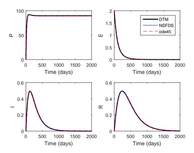
Fig. 3: Numerical simulation of the model for disease-free equilibrium using Differential Transformation Method (solid black), Non Standard Finite Difference Scheme (solid blue) and ode45 MATLAB routine (dashed red). Here we use the time step of 0.01 for the DTM and NSFDS and error tolerance of 10−5 for MATLAB ode45 routine.
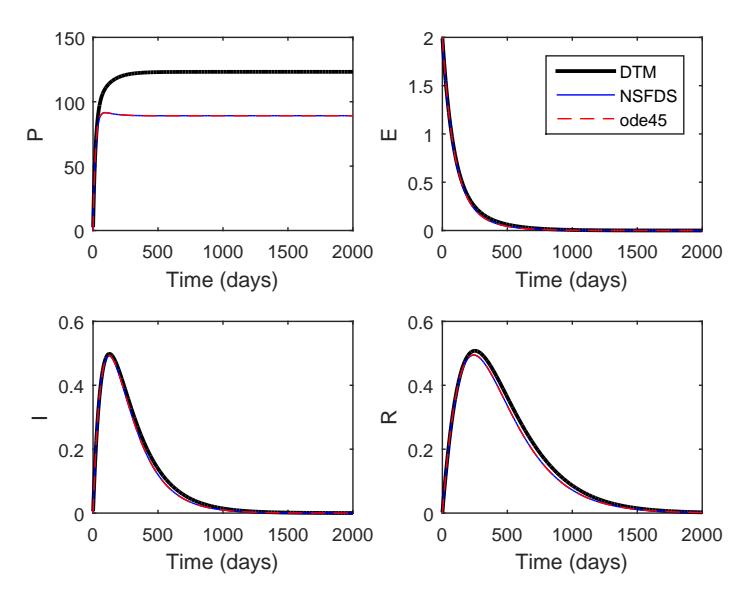
Fig. 4: Numerical simulation of the model for disease-free equilibrium using Differential Transformation Method (solid black), Non Standard Finite Difference Scheme (solid blue) and ode45 MATLAB routine (dashed red). Here we use the time step of h=0.5 for the DTM and NSFDS and error tolerance of 10−5 for MATLAB ode45 routine.
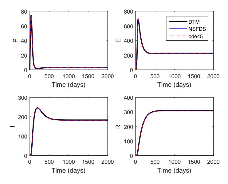
Fig. 5: Numerical simulation of the model for endemic equilibrium using Differential Transformation Method (solid black), Non Standard Finite Difference Scheme (solid blue) and MATLAB ode45 routine (dashed red). Here we use the time step of 0.01 for the DTM and NSFDS and error tolerance of 10−5 for MATLAB ode45 routine.
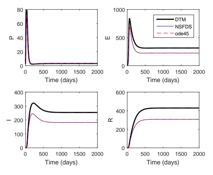
Fig. 6: Numerical simulation of the model for endemic equilibrium using Differential Transformation Method (solid black), Non Standard Finite Difference Scheme (solid blue) and MATLAB ode45 routine (dashed red). Here we use the time step of 0.5 for the DTM and NSFDS and error tolerance of 10−5 for MATLAB ode45 routine.
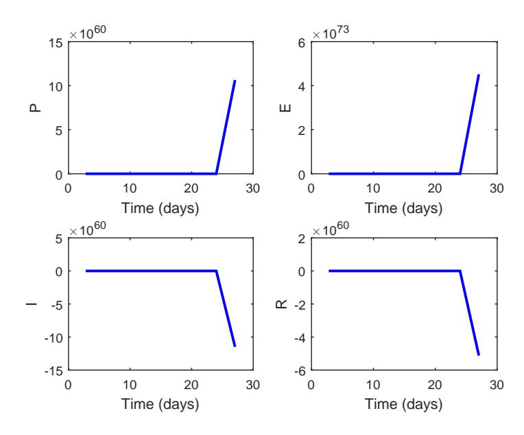
Fig. 7: Numerical simulation of the model for endemic equilibrium using Differential Transformation Method with the time step of three.
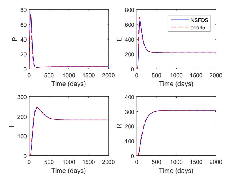
Fig. 8: Numerical simulation of the model for endemic equilibrium using Non Standard Finite Difference Scheme (solid blue) and MATLAB ode45 routine (dashed red). Here we use the time step of 3 for the NSFDS and error tolerance of 10−5 for MATLAB ode45 routine.
Figures 5 and 6 show numerical simulations of endemic equilibrium point using these three methods. We found similar results as that for disease-free equilibrium. The DTM and NSFDS agree well with MATLAB ode45 if the time steap is 0.01 but the DTM gives different results if the time step is 0.5. Furthermore, if we increase the time step, the DTM cannot converge and fails in generating the model's solutions (see Figure 7), whereas the NSFDS and MATLAB ode45 routine converge and give similar solution (see Figure 8). It is clear that when the time step is large (h = 3), the numerical solutions generated by NSFDS still performs better than that of the DTM.
6. DISCUSSIONS
In this paper, the DTM and NSFDS are constructed to simulate a mathematical model of plant disease transmission. The simulation results are then compared to the well-established MATLAB ode45 routine. It shows that the solutions of the DTM and NSFDS give similar results to the MATLAB ode45 routine for the small time step. However, when the time step increases, the performance of NSFDS is better than that of the DTM. This confirms the previous findings that the DTM performs well in the small time step. If the time step is larger, the DTM may not converge [26]. On the other hand, the NSFDS can perform well in the large time step [15], [19]. Although the time domain is divided into m sub domain and the solutions is obtained from each domain [26], the chosen time step still play important role in determining the accuracy of the solutions generated by the DTM. There are also other variants of the DTM that may provide different results in terms of accuracy [25], [28], [13], [11] but this is not the focus of the paper. Interested readers can employ other variants of the DTM and compare the results to the NSFDS. Our findings suggest that the NSFSD may be the first choice when the standard numerical methods fail in generating the solution of the model.
7. CONCLUSION
In this paper, we compare the numerical results of differential transformation method and non standard finite difference scheme. We found that the result nonstandard finite difference scheme performs well in comparison to the differential transformation method in particular for the large timestep h. Nonstandard finite difference scheme can be an alternative for solving a system of differential equations when the traditional methods such as Runge-Kutta fail in generating solutions.
ACKNOWLEDGEMENT
MZN acknowledges funding from Ministry of Research, Technology and Higher Education of Indonesia 2018 (Grant No: 70/ UN15.19 /LT /2018). NA received Academic Leadership Grant from Padjadjaran University (Grant No:2297 /UN6.D /KS /2018) and Penelitian Dasar Unggulan Perguruan Tinggi (Grant No: 1126/UN6.D/LT/2018).