

1. Introduction
HIV (Human Immunodeficiency Virus) attacks the host cells expressing CD4<sup>+</sup> molecule, the majority is CD4<sup>+</sup> T cells [1]. These cells play the main role in spreading HIV-1 infection within host cells. The transmission of HIV in the immune system can occur through the contact of infected host cells or free virus to healthy cells. Even viral transmission from infected host cells results the effective infection compared to viral transmission via a free virus. [2], [3], [4].
Infected CD4<sup>+</sup> T cells stimulate cytotoxic T-lymphocytes (CTL) cells. Cytotoxic (CD8<sup>+</sup>) cells are effector cell that inhibits viral replication and eliminate by combating the infected cells. CD8<sup>+</sup> T cells have an important role in controlling HIV infection due to the elimination of infected cells forming viral replication [5].
The process of viral reverse transcription that transcribes viral RNA to host DNA determines viral infection in target cells. Upon incomplete transcription within the host cell, \(CD4^+\) T cells are able to degrade virus in the cytoplasm and return to healthy state. Otherwise, upon complete reverse transcription occurred in host cells, these cells become infectious and produce new viral particles to infect the target cells [6].
CD4<sup>+</sup> T cells have a critical role in HIV-1 infection. The stimulated CD4<sup>+</sup> T cells are able to create a productive infection. On the other hand, the resting cells are able to prevent the process of viral reverse transcription and lead to infection failure due to incomplete reverse transcription. The virus is degraded by resting cells [7], [9], [8].
Recently, the treatments of RTI (reverse transcript inhibitor) and PI (protease inhibitor) have been used to prevent HIV-1 infection for infected patients. RTI drugs function to block the mechanism of viral reverse transcription, while PI drugs block new viral reproduction from infected CD4<sup>+</sup> T cells. The therapy has been conducted in preventing viral DNA synthesis and new viral production [7].
Some studies have been established regarding HIV-1 infections in host cells. A model was proposed by Srivastava et al.. The model was established by considering on viral reverse transcription in the infection process of CD4<sup>+</sup> T cells [10]. Upon reverse transcription in CD4<sup>+</sup> T cells, these cells are classified into two sub populations, namely pre-RT and post-RT classes. They studied the effect of RTI treatment. Instead, they have not considered the infection by cell to cell contact cell as well as PI treatment.
A model was proposed by Chirove et al. [11] and Sutimin et al. [12], [13], to capture HIV-1 the infection of Langerhans and CD4<sup>+</sup> T cells in early HIV-1 infection. Chirove et al. used the behavior of alternative
reproduction ratio to analyze the dynamics of the model. A model by considering the effect of RTI and PI drugs was proposed by Sutimin et.al to study the immune response of drugs in HIV-1 infection [12], [13].
Other studies, Tarfulea et al. established a model accommodating CTL cells and antiretroviral treatment in reducing HIV-1 infection [14], [15]. They investigated numerically the effect of CTL response and treatment of RTI and PI combination in controlling virus during early infection. The results show that the CTL response is more significant in increasing healthy CD4<sup>+</sup> T cells compared to therapy.
We develop the model's Srivastava by incorporating HIV transmission through cell to cell, the effect of PI drug and CTL compartment. We analyze the model to determine the existence and stability of equilibria, as well as viral clearance effect of CD4<sup>+</sup> T cells. We investigate numerically the implication of RTI and PI treatment in various scenarios to find the effectiveness of drugs.
2. MODEL FORMULATION
We develop a model by considering HIV-1 transmission from the interaction between infected and healthy CD4<sup>+</sup> T cells, the effectiveness of RTI and PI drugs, and the compartment of CTL cells. The HIV-1 transmission in CD4<sup>+</sup> T cells can be presented in the following diagram.
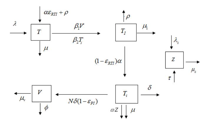
Fig. 1: Diagram HIV-1 transmission within CD4<sup>+</sup> T cells with CTL cells response.
Upon HIV-1 fusion within CD4<sup>+</sup> T cells, these cells are classified into two classes, namely pre-RT class and post-RT (actively infected) class. The population of pre-RT class, in which the process of RT is not efficient, denoted by \(T_1\). The population of post-RT class, in which the process of RT is complete, denoted by \(T_i\). The population of susceptible CD4<sup>+</sup> T cells is denoted by \(T_i\), the population of CTL cells, denoted by \(T_i\), and the population of free virus is denoted by \(T_i\). The model is given as follows.
\[\frac{dT}{dt} = \lambda - \beta_1 V T - \beta_2 T T_i - \mu T + (\epsilon_{RTI} \alpha + \rho) T_1,\] \[\frac{dT_1}{dt} = \beta_1 T V + \beta_2 T T_i - (\mu_1 + \alpha + \rho) T_1,\] \[\frac{dT_i}{dt} = (1 - \epsilon_{RTI}) \alpha T_1 - (\mu + \delta) T_i - \omega T_i Z,\] \[\frac{dZ}{dt} = \lambda_z + \tau T_i - \mu_z Z,\] \[\frac{dV}{dt} = N\delta (1 - \epsilon_{PI}) T_i - \mu_v V - \phi V.\] (1)
The population of CD4<sup>+</sup> T cells are produced by thymus with constant rate \(\lambda\), and die naturally at a rate \(\mu\). Infection by a free virus and infected CD4<sup>+</sup> T cells are at constant rates \(\beta_1\) and \(\beta_2\), respectively. Upon RTI treatment and the process of inefficient reverse transcription, pre-RT class return to healthy CD4<sup>+</sup> T cells with the constant rates \(\epsilon_{RTI}\alpha + \rho\). The incomplete reverse transcription leads to inflammation of pre-RT
CD4<sup>+</sup> T cells, assumed that this population dies at a constant rate \(\mu_1\), due to the inflammation. Due to RTI treatment, a part of \(\epsilon_{RTI}\alpha T_1\) of pre-RT population back to susceptible, while other part, \((1 - \epsilon_{RTI}) \alpha T_1\) become infectious, and pre-RT class move to post-RT class at a rate \((1 - \epsilon_{RTI}) \alpha\). Infected CD4<sup>+</sup> T cells are killed by CTL cells with the constant rate \(\omega\).
The recruitment of CTL cells is assumed at constant rate \(\lambda_z\). Due to the immune response of infected CD4<sup>+</sup> T cells, the proliferation of the CTL cells increase at a constant rate \(\tau\), and these cells die at the rate \(\mu_z\). Due to PI treatment, new viral produced by infected CD4<sup>+</sup> T cells reduce becoming \(N\delta\) (1 – \(\epsilon_{PI}\)). The viral death rate and viral clearances level are \(\mu_v\) and \(\phi\), respectively. The efficacy values of RTI and PI drugs are denoted by \(\epsilon_{RTI}\) and \(\epsilon_{PI}\), respectively with \(0 \le \epsilon_{RTI}\), \(\epsilon_{PI} \le 1\).
3. MODEL ANALYSIS
We analyze the existence of the endemic equilibrium point and the stability of equilibria for the model.
3.1. Alternative reproduction ratio
The alternative reproduction ratio is derived from the next generation matrix. The next generation matrix [16] of the Model 1 is given by
\[G = \begin{bmatrix} 0 & \frac{\beta_2 \lambda \mu_z}{\mu(\delta \mu_z + \lambda_z \omega + \mu \mu_z)} & \frac{\beta_1 \lambda}{\mu(\phi + \mu_v)} \\ \frac{(1 - \epsilon_{RTI})\alpha}{\mu_1 + \alpha + \rho} & 0 & 0 \\ 0 & \frac{N\delta (1 - \epsilon_{PI})\mu_z}{\delta \mu_z + \lambda_z \omega + \mu \mu_z} & 0 \end{bmatrix}.\] (2)
The characteristic polynomial corresponding to matrix G can be expressed as
\[P(X) = X^3 - B_1 X - B_0, (3)\] where
\[\begin{split} B_1 &= \frac{\alpha \, \beta_2 \, (1 - \epsilon_{RTI}) \, \lambda \mu_z}{\left(\delta \, \mu_z + \lambda_z \omega + \mu \mu_z\right) \mu \, \left(\mu_1 + \alpha + \rho\right)}, \\ B_0 &= \frac{\mu_z \lambda \, (1 - \epsilon_{RTI}) \, (1 - \epsilon_{PI}) \, \beta_1 \delta \, \alpha \, N}{\left(\mu_1 + \alpha + \rho\right) \mu \, \left(\phi + \mu_v\right) \left(\delta \, \mu_z + \lambda_z \omega + \mu \mu_z\right)}. \end{split}\]
The basic reproduction number \(\Re_0\) cannot be formulated explicitly. Instead, we can determine alternative reproduction ratio, denoted \(\Re_1\) which is equivalent to \(\Re_0\). The alternative reproduction ratio is defined by \(\Re_1^2 = B_0 + B_1\) (see [11]) that can be expressed as \(\Re_0 = \Re_{T_i \mapsto T_i} + \Re_{T_i \mapsto V_i}\), where
\[\begin{split} \Re_{T_i \mapsto T_i} & = & \frac{\beta_2 \alpha \, \left(1 - \epsilon_{RTI}\right) \lambda \mu_z}{\left(\delta \, \mu_z + \lambda_z \omega + \mu \mu_z\right) \mu \, \left(\mu_1 + \alpha + \rho\right)}, \\ \Re_{T_i \mapsto V \mapsto T_i} & = & \frac{\mu_z \lambda \, \left(1 - \epsilon_{RTI}\right) \left(1 - \epsilon_{PI}\right) \beta_1 \delta \, \alpha \, N}{\left(\mu_1 + \alpha + \rho\right) \mu \, \left(\phi + \mu_v\right) \left(\delta \, \mu_z + \lambda_z \omega + \mu \mu_z\right)}. \end{split}\]
As in [11], [12], [13], sub-ratio \(\Re_{T_i \mapsto T_i}\) indicates the infection path from an infected CD4<sup>+</sup> T cell to healthy CD4<sup>+</sup> T cells. Sub-ratio \(\Re_{T_i \mapsto V \mapsto T_i}\) indicates the infection path from infected CD4<sup>+</sup> T cell then reproduces new viral particles infecting healthy CD4<sup>+</sup> T cells. The relation of basic reproduction ratio \((\Re_0)\) and \(\Re_1\) was given the following Theorem 3.1.
Theorem 3.1. The reproduction ratio, \(\Re_0\) and alternative reproduction ratio, \(\Re_1\) for system 1 hold the equivalent properties as follows.
- i. \(\Re_0 = 1\) if only if \(\Re_1 = 1\).
- ii. \(\Re_0 < 1\) if only if \(\Re_1 < 1\), and \(\Re_0 > 1\) if only if \(\Re_1 > 1\).
Proof: First, we show that Eq. (3) has only one positive real root with the largest modulus. Let \(x_1, x_2\)and \(x_3\) be the roots of polynomial in Eq. (3), then it holds
\[x_1 + x_2 + x_3 = 0, (4)\]
\[x_1x_2 + x_1x_3 + x_2x_3 = -B_1 < 0, (5)\]
\[x_1 x_2 x_3 = B_0 > 0. (6)\]
From Eq. (4) and Eq. (6), the polynomial equation has only real positive one root and two negative real roots or two complex roots with negative real parts. Next, we show that one positive real root has the largest modulus.
Case 1: For one positive root and two negative real roots. Without loss of the generality, let \(x_1 > 0\) and \(x_2, x_3 < 0\). From Eq. (4), we have \(x_1 = -x_2 - x_3 > 0\). Thus \(|x_1| > |x_2|\) and \(|x_1| > |x_3|\).
Case 2: For one positive root and two complex roots. Let \(x_1 > 0\), \(x_2 = ai + b\), and \(x_3 = ai - b\). From Eq. (5), it can be written as \(x_1(x_2 + x_3) + a^2 + b^2 = -B_1\), thus
\[2ax_1 + a^2 + b^2 = -B_1 < 0 (7)\]
On the other hand, from Eq. (4), we have \(x_1 + 2a = 0\) or \(a = -\frac{x_1}{2}\). Thus, the Equation (7) can be written as
\[-x_1^2 + a^2 + b^2 = -B_1 < 0 (8)\]
From the Equation (8), we have \(x_1^2 > a^2 + b^2\). It is shown that the polynomial in Eq. (3) has exactly one positive real root that has the largest modulus. Next, we prove i. as follows. When \(\Re_0=1\), then it holds P(1)=0. It means \(1-B_1-B_0=0\). Thus \(B_1+B_0=1=\Re_1\). Conversely, if \(\Re_1=1\), then \(1=B_1+B_0\) or \(1-B_1-B_0=0\). It means P(1)=0, thus \(\Re_0=1\). The proof ii. is as follows. Let \(\Re_0<1\), then it holds
\[P(\Re_0) \equiv \Re_0^3 - B_1 \Re_0 - B_0 = 0 \tag{9}\]
The Equation (9) can be written as
\[\Re_0 \left( \Re_0^2 - B_1 \right) = B_0,\] \[= \Re_1^2 - B_1, \text{ since } \Re_1^2 = B_1 + B_0.\] (10)
\[= \Re_1^2 - B_1, \text{ since } \Re_1^2 = B_1 + B_0. \tag{11}\]
Since \(\Re_0 > 1\), we have \(\Re_1^2 - B_1 = \Re_0 \left(\Re_0^2 - B_1\right) > \Re_0^2 - B_1\). It means that \(\Re_1^2 > \Re_0^2 > 1\), thus \(\Re_1 > 1\). By contrapositive, if \(\Re_1 > 1\) then \(\Re_0 > 1\), it means if \(\Re_0 \le 1\) then \(\Re_1 \le 1\). The proof, if \(\Re_0 = 1\) then \(\Re_0 = 0\), is given in (i). Now, let \(\Re_0 < 1\), from Eq. (9), we have \(\Re_1^2 - B_1 = \Re_0 \left(\Re_0^2 - B_1\right) < \Re_0^2 - B_1\). It is obtained \(\Re_1^2 < \Re_0^2 < 1\), thus \(\Re_1 < 1\). The second statement of (ii) is proven similarly. It completes the proof.
3.2. Stability analysis of uninfected steady state
Uninfected equilibrium point is \(E^0 = (T^0, T^0_1, T^0_i, Z^0, V^0) = (\frac{\lambda}{\mu}, 0, 0, \frac{\lambda_z}{\mu_z}, 0)\). The local stability of \(E^0\) is given in the following theorem.
Theorem 3.2. The uninfected equilibrium point \(E^0\) is locally asymptotically stable, if \(\Re_1 < 1\).
Proof: The Jacobian matrix of the model 1 at \(E^0\) can be written b
\[J(E^{0}) = \begin{bmatrix} -\mu & \alpha \, \epsilon_{RTI} + \rho & -\frac{\beta_{2}\lambda}{\mu} & 0 & -\frac{\lambda\beta_{1}}{\mu} \\ 0 & -\mu_{1} - \alpha - \rho & \frac{\beta_{2}\lambda}{\mu} & 0 & \frac{\lambda\beta_{1}}{\mu} \\ 0 & (1 - \epsilon_{RTI}) \alpha & -\frac{\lambda_{z}\omega}{\mu_{z}} - \delta - \mu & 0 & 0 \\ 0 & 0 & \tau & -\mu_{z} & 0 \\ 0 & 0 & N\delta \, (1 - \epsilon_{PI}) & 0 & -\phi - \mu_{v} \end{bmatrix}.\](12)
The eigenvalues of \(J(E^0)\) are \(-\mu, -\mu_z\), and others are solutions of the cube equation
\[\lambda^3 + A_2 \lambda^2 + A_1 \lambda + A_0 = 0, (13)\]
where
\[A_{2} = \alpha + \delta + \phi + \rho + \mu_{1} + \mu + \mu_{v} + \frac{\lambda_{z}\omega}{\mu_{z}},\] \[A_{1} = \frac{1}{\mu_{z}} \left( 1 - \Re_{1}^{2} \right) (\mu_{1} + \alpha + \rho) \left( \delta \mu_{z} + \lambda_{z}\omega + \mu \mu_{z} \right)\] \[+ \frac{\lambda \left( 1 - \epsilon_{RTI} \right) \alpha N \delta \left( 1 - \epsilon_{PI} \right) \beta_{1}}{\mu \left( \phi + \mu_{v} \right)} + \frac{(\phi + \mu_{v}) \omega \lambda_{z}}{\mu_{z}}\] \[+ (\phi + \mu_{v}) \left( \alpha + \delta + \rho + \mu_{1} + \mu \right),\] \[A_{0} = \frac{1}{\mu_{z}} \left( 1 - \Re_{1}^{2} \right) (\mu_{1} + \alpha + \rho) \left( \delta \mu_{z} + \lambda_{z}\omega + \mu \mu_{z} \right) (\phi + \mu_{v}).\]
It is seen that \(A_2, A_1 > 0\) if \(\Re_1 < 1\). Next, we calculate \(A_2A_1 - A_0\). Manipulating calculation, it is obtained
\[A_{2}A_{1} - A_{0} = \frac{(\delta \mu_{z} + \lambda_{z}\omega + \mu\mu_{z})(\mu_{1} + \alpha + \rho)\Psi_{1}(1 - \Re_{\theta})}{\mu_{z}^{2}} + \frac{N\alpha \delta (1 - \epsilon_{PI})(1 - \epsilon_{RTI})\lambda\Psi_{2}\beta_{1}}{\mu_{z}\mu(\phi + \mu_{v})} + \frac{(\phi + \mu_{v})\Psi_{1}\Psi_{2}}{\mu_{z}^{2}},\] (14)
where
\[\Psi_1 = (\alpha + \delta + \rho + \mu_1 + \mu) \mu_z + \lambda_z \omega, \Psi_2 = (\alpha + \delta + \phi + \rho + \mu_1 + \mu + \mu_v) \mu_z + \lambda_z \omega.\]
The Routh-Hurwitz criterion is fulfilled when \(\Re_1 < 1\). It shows that \(E^0\) locally asymptotically stable.
3.3. The existence and uniqueness of endemic equilibrium
The endemic equilibrium point of the model is \(E^* = (T^*, T_1^*, T_i^*, Z^*, V^*)\), where
\[T^{*} = \frac{\omega \tau (\phi + \mu_{v}) (\mu_{1} + \alpha + \rho) T_{i}^{*}}{\alpha (1 - \epsilon_{RTI}) \mu_{z} (N \delta \beta_{1} (1 - \epsilon_{PI}) + \beta_{2} \phi + \beta_{2} \mu_{v})} + \frac{(\phi + \mu_{v}) (\delta \mu_{z} + \lambda_{z} \omega + \mu \mu_{z}) (\mu_{1} + \alpha + \rho)}{\alpha (1 - \epsilon_{RTI}) \mu_{z} (N \delta \beta_{1} (1 - \epsilon_{PI}) + \beta_{2} \phi + \beta_{2} \mu_{v})},\] \[T_{1}^{*} = \frac{T_{i}^{*} (T_{i}^{*} \omega \tau + \delta \mu_{z} + \lambda_{z} \omega + \mu \mu_{z})}{\alpha (1 - \epsilon_{RTI}) \mu_{z}},\] \[Z^{*} = \frac{\tau T_{i}^{*} + \lambda_{z}}{\mu_{z}},\] \[V^{*} = \frac{N T_{i}^{*} \delta (1 - \epsilon_{PI})}{\phi + \mu_{v}}.\]
The value of \(T_i^*\) is the positive root of a quadratic equation
\[b_2 T_i^2 + b_1 T_i + b_0 = 0, (15)\] where
\[\begin{array}{lll} b_{2} & = & \omega\,\tau\,\left(\left(1-\epsilon_{RTI}\right)\alpha+\mu_{1}\right)\left(N\delta\,\beta_{1}\left(1-\epsilon_{PI}\right)+\beta_{2}\phi+\beta_{2}\mu_{v}\right)>0,\\ b_{1} & = & N\delta\,\left(1-\epsilon_{PI}\right)\left(\delta\,\mu_{z}+\lambda_{z}\omega+\mu\mu_{z}\right)\left(\left(1-\epsilon_{RTI}\right)\alpha+\mu_{1}\right)\beta_{1}\\ & & +\left(\phi+\mu_{v}\right)\left(\delta\,\mu_{z}+\lambda_{z}\omega+\mu\mu_{z}\right)\left(\left(1-\epsilon_{RTI}\right)\alpha+\mu_{1}\right)\beta_{2}\\ & & +\omega\,\tau\,\mu\left(\phi+\mu_{v}\right)\left(\mu_{1}+\alpha+\rho\right),\\ b_{0} & = & \mu\left(\mu_{1}+\alpha+\rho\right)\left(\delta\,\mu_{z}+\lambda_{z}\omega+\mu\mu_{z}\right)\left(\phi+\mu_{v}\right)\left(1-\Re_{I}^{2}\right). \end{array}\]
Due to \(b_2 > 0\), Eq. (15) has exactly one positive root if only if \(b_0 < 0\), it is fulfilled when \(\Re_1 > 1\).
We investigate the parameter \(\Re_1\) due to the effect of viral lysis corresponding to the critical number of viral production for the endemicity of HIV-1 infection. Differentiating \(\Re_1^2\) with respect to \(\delta\) is obtained as follows,
\[\frac{\partial \Re_{1}^{2}}{\partial \delta} = \frac{\left(1 - \epsilon_{RTI}\right) \alpha \lambda \mu_{z} \beta_{1} \left(1 - \epsilon_{PI}\right) \left(\lambda_{z} \omega + \mu \mu_{z}\right) \left(N - N_{c}\right)}{\mu \left(\mu_{1} + \alpha + \rho\right) \left(\delta \mu_{z} + \lambda_{z} \omega + \mu \mu_{z}\right)^{2} \left(\phi + \mu_{v}\right)},\tag{16}\] where
\[N_c = \frac{\beta_2 \mu_z \left(\phi + \mu_v\right)}{\beta_1 \left(1 - \epsilon_{PI}\right) \left(\lambda_z \omega + \mu \mu_z\right)}.\] (17)
The quantity \(N_c\) is defined as the critical viral production of infected CD4<sup>+</sup> T cells. From this result, the relationship between N and \(N_c\) is given in the following theorem.
Theorem 3.3. The critical number \(N_c\) determines the endemicity level of HIV-1 infection as follows
- i. The level of \(\Re_1\) decreases with respect to \(\delta\), when \(N < N_c\).
- ii. The level of \(\Re_1\) increase with respect to \(\delta\), when \(N > N_c\), and
- iii. The level of \(\Re_1\) remains constant with respect to \(\delta\), when \(N=N_c\).
Proof: When \(N < N_c\), it implies that \(\frac{\partial \Re_1^2}{\partial \delta} < 0\), so \(\Re_1\) decreases with respect to \(\delta\). But when \(N > N_c\), it implies \(\frac{\partial \Re_1^2}{\partial \delta} > 0\), it means that \(\Re_1\) increases with respect to \(\delta\). For \(N = N_c\), implies \(\frac{\partial \Re_1^2}{\partial \delta} = 0\). It shows that \(\Re_1\) remains constant with respect to \(\delta\).
3.4. The stability of endemic equilibrium
We use Lyapunov function to analyze global stability of endemic equilibrium. The global stability is given in the following Theorem.
Theorem 3.4. The endemic equilibrium point \(E^0\) is globally asymptotically stable, if \(\Re_1 > 1\).
Proof: We construct a Lyapunov function as follows,
\[L(T, L, T_{i}, V) = T - T^{*} - T^{*} \ln\left(\frac{T}{T^{*}}\right) + c_{1}\left(T_{1} - T_{1}^{*} - L^{*} \ln\left(\frac{T_{1}}{T_{1}^{*}}\right)\right) + c_{2}\left(T_{i} - T_{i}^{*} - T_{i}^{*} \ln\left(\frac{T_{i}}{T_{i}^{*}}\right)\right) + c_{3}\left(Z - Z^{*} - Z^{*} \ln\left(\frac{Z}{Z^{*}}\right)\right) + c_{4}\left(V - V^{*} - V^{*} \ln\left(\frac{V}{V^{*}}\right)\right),\] \[(18)\] where \(c_1, c_2, c_3\) and \(c_4\) are positive constants that must be determined. It is shown \(F \in C^1\), \(F(E^*) = 0\). Differentiating F due to t in along solutions, we obtain
\[\frac{dL}{dt} = \frac{T - T^*}{T} \frac{dT}{dt} + a_1 \frac{T_1 - T_1^*}{T_1} \frac{dT_1}{dt} + c_2 \frac{T_i - T_i^*}{T_i} \frac{dT_i}{dt} + c_3 \frac{Z - Z^*}{Z} \frac{dZ}{dt} + c_4 \frac{V - V^*}{V} \frac{dV}{dt} = K - \mu T + [A_0 - c_1 A_1 + c_2 (1 - \epsilon_{RTI}) \alpha] T_1 + [c_2 \omega T_i^* - c_3 \mu_z] Z + [\beta_2 T^* - c_2 A_2 + c_3 \tau + a_4 (1 - \epsilon_{PI} N \delta)] T_i + [\beta_1 T^* - c_4 A_3] V + [c_1 \beta_1 - \beta_1] V T + [c_1 \beta_2 - \beta_2] T T_i - c_2 \omega T_i Z - \lambda \frac{T^*}{T} - A_0 T^* \frac{T_1}{T} - c_1 \beta_1 L^* \frac{TV}{T_1} - c_1 \beta_2 L^* \frac{TT_i}{T_1} - c_2 (1 - \epsilon_{RTI}) \alpha T_i^* \frac{T_1}{T_i} - c_3 \lambda_z \frac{Z^*}{Z} - c_3 \tau Z^* \frac{T_i}{Z} - c_4 (1 - \epsilon_{PI}) N \delta V^* \frac{T_i}{V},\] (19)
where \(K=\lambda+\mu T^*+c_1A_1T_1^*+c_2A_2T_i^*+c_3\mu_zZ^*+c_4A_3V^*+c_3\lambda_z\), with \(A_0=\epsilon_{RTI}\alpha+\rho\), \(A_1=\mu_1+\alpha+\rho\), \(A_2=\mu+\delta\) and \(A_3=\mu_v+\phi\). We let the new notations, \(x=\frac{T}{T^*},y=\frac{L}{L^*},w=\frac{T_i}{T_i^*},z=\frac{Z}{Z^*}\) and \(u=\frac{V}{V^*}\). The Equation (19) becomes
\[\frac{dL}{dt} = K - \mu T^* x + [A_0 - c_1 A_1 + c_2 (1 - \epsilon_{RTI}) \alpha] T_1^* y + [c_2 \omega T_i^* - c_3 \mu_z] Z^* z [\beta_2 T^* - c_2 A_2 + c_3 \tau + a_4 (1 - \epsilon_{PI} N \delta)] T_i^* w + [\beta_1 T^* - c_4 A_3] V^* u + [c_1 \beta_1 - \beta_1] V^* T^* x u + [c_1 \beta_2 - \beta_2] T^* T_i^* x w - c_2 \omega T_i^* Z^* z w - \lambda \frac{1}{x} - A_0 T_1^* \frac{y}{x} - c_1 \beta_1 T^* V^* \frac{xu}{y} - c_1 \beta_2 T^* T_i^* \frac{xw}{y} - c_2 (1 - \epsilon_{RTI}) \alpha T_1^* \frac{y}{w} - c_3 \lambda_z \frac{1}{z} - c_3 \tau T_i^* \frac{w}{z} - c_4 (1 - \epsilon_{PI}) N \delta T_i^* \frac{w}{z}.\] (20)
We construct a variable set, \(D = \left\{x, y, z, w, u, xw, xu, zw, \frac{1}{x}, \frac{1}{z}, \frac{y}{x}, \frac{w}{u}, \frac{xz}{y}, \frac{xu}{y}, \frac{xw}{y}\right\}\) related to terms in Eq. (20). There are three sub sets of D, in which the product of elements is unity, namely \(\left\{x, \frac{1}{x}\right\}\), \(\left\{\frac{1}{x}, \frac{y}{w}, \frac{xw}{y}\right\}\) and \(\left\{\frac{1}{x}, \frac{y}{w}, \frac{w}{u}, \frac{xu}{y}\right\}\). Equating coefficients of y, w, u, z, xu, xw to zero in Eq. (20). The Equation (20) can be constructed as follows,
\[\frac{dL}{dt} = b_1 \left( 2 - x - \frac{1}{x} \right) + b_2 \left( 2 - z - \frac{1}{z} \right) + b_3 \left( 3 - \frac{1}{x} - \frac{y}{w} - \frac{xw}{y} \right) + b_4 \left( 4 - \frac{1}{x} - \frac{y}{w} - \frac{w}{u} - \frac{xu}{y} \right) - c_2 \omega T_i^* Z^* z w - A_0 L^* \frac{y}{x} - c_3 \tau T_i^* \frac{w}{z}.\] (21)
The constants \(b_1, b_2, b_3, a_1, a_2, a_3\) can be obtained with considering the relation
\[\begin{array}{rcl} \lambda + (\epsilon_{RTI}\alpha + \rho)\,T_1^* & = & \beta_1 T^*V^* + \beta_2 T^*T_i^* + \mu\,T^*, \\ \beta_1 T^*V^* + \beta_2 T^*T_i^* & = & (\mu_1 + \alpha + \rho)\,L^*, \\ (\mu + \delta)\,T_i^* + \omega T_i^*Z^* & = & (1 - \epsilon_{RTI})\,\alpha L^*, \\ \mu_z Z^* & = & \lambda_z + \tau T_i^*, \\ (\mu_v + \phi)\,V^* & = & N\delta\,(1 - \epsilon_{PI})\,T_i^*. \end{array}\]
Equating coefficients in the similar terms of Equation (20) and (21), we get, \(2b_1 + 2b_2 + 3b_3 + 4b_4 = K, \ c_1 - 1 = 0, \ b_1 = \mu T^*, \ b_2 = c_3\mu_z - c_2\omega T_i^* = c_3\lambda_z, \\ b_1 + b_2 + b_3 = \lambda, \ b_3 + b_4 = c_2\left(1 - \epsilon_{RTI}\right)\alpha T_1^*, \ b_3 = c_1\beta_2 T^*T_i^* \\ b_3 + b_4 = c_2\left(1 - \epsilon_{RTI}\right)\alpha T_1^*, \ b_4 = c_4\left(1 - \epsilon_{PI}\right)N\delta T_i^* = c_1\beta_1 V^*T^*. \text{ We can choose } c_1 = 1, \ c_2 = \frac{A_1T_1^*}{(1 - \epsilon_{RTI})\alpha T_1^*}, \ c_3 = \frac{\omega A_1T_1^*T_i^*}{(1 - \epsilon_{PI})(\mu_z - \lambda_z)} \text{ and } c_4 = \frac{\beta_1 V^*T^*}{(1 - \epsilon_{PI})N\delta T_i^*}. \text{ Considering the inequality of arithmetic and geometric mean, the Equation 21 can be written by}\)
\[\begin{split} \frac{dL}{dt} &= \mu T^* \left( 2 - x - \frac{1}{x} \right) + \frac{\omega \lambda_z A_1 T_1^* T_i^*}{(1 - \epsilon_{PI}) \left( \mu_z - \lambda_z \right)} \left( 2 - z - \frac{1}{z} \right) + \\ & \beta_2 T^* V^* \left( 3 - \frac{1}{x} - \frac{y}{w} - \frac{xw}{y} \right) + \beta_1 T^* V^* \left( 4 - \frac{1}{x} - \frac{y}{w} - \frac{w}{u} - \frac{xu}{y} \right) \\ & - A_0 T_1^* \frac{y}{x} - \frac{\omega A_1 T_1^* T_i^* Z^*}{(1 - \epsilon_{RTI}) \alpha T_1^*} zw - \frac{\omega \tau A_1 T_1^* T_i^*}{(1 - \epsilon_{RTI}) \alpha T^* \left( \mu_z - \lambda_z \right)} \frac{w}{z} \le 0. \end{split}\]
It can be seen that \(\frac{dL}{dt}=0\) when \(T=T^*, T_1=T_1^*, T_i=T_i^*, Z=Z^*\) and \(V=V^*\) thus the maximal invariance set of \(\left\{(T,T_1,T_i,Z,V)\,|\frac{dL}{dt}=0\right\}\) is the singleton \(E^*\). Thus \(E^*\) indicates globally asymptotically stable. The proof is completed.
4. NUMERICAL SIMULATIONS
In the section, we present the simulation results regarding to evolutions of CD4<sup>+</sup> T cells, CTL cells, and viral free populations to investigate the impact of combining RTI and PI treatments. The parameter values used in the simulations are determined from literature as given in Table I.
| Parameters | Values | Units | References |
|---|---|---|---|
| λ | 10, 20 | cells day-1 | [18], [22] |
| \(\lambda_z\) | 0.0001 | cells day-1 | [21] |
| \(\tilde{\tau}\) | 0.1 | day-1 | [23] |
| \(\alpha\) | 0.4 | day-1 | [10] |
| \(\beta_1\) | (0.00002, 0.005) | virions-1day-1 | [19], [20] |
| ρ | 0.05 | day-1 | [10] |
| \(\omega\) | 0.01 | day-1 | [21] |
| \(\beta_2\) | (0.00001, 0.01) | cells-1day-1 | [11] |
| \(\mu\) | 0.01, 0.02 | day-1 | [18], [22] |
| \(\mu_1\) | 0.015 | day-1 | [10] |
| \(\mu_z\) | 0.1, 0.2 | day-1 | [14], [24] |
| \(\mu_v\) | 2.4 | day-1 | [18] |
| δ | 0.24 | day-1 | [18] |
| N | (100, 1000) | virions day-1 | [21] |
| \(\phi\) | (2,9) | day-1 | [18] |
TABLE I: The values of parameter and units
We simulate the evolution of CD4<sup>+</sup> T cells, CTL cells, and virus populations to investigate numerically the effect of RTIs and PIs treatments. The initial conditions are taken \(T(0)=850 \frac{cells}{mm^3}\), \(T_1(0)=40 \frac{cells}{mm^3}\), \(T_1(0)=40 \frac{cells}{mm^3}\), and \(T_1(0)=40 \frac{cells}{mm^3}\). [26]. Next, we shall investigate the clearance effect of the virus to the dynamic of CD4<sup>+</sup> T cells and free virus population.
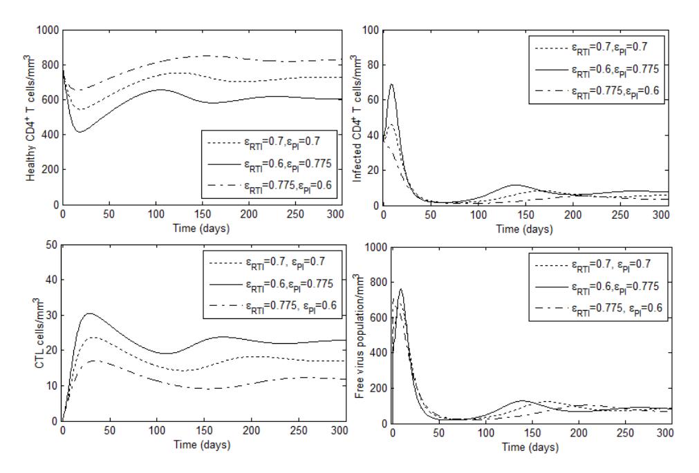
Fig. 2: The evolution of CD4<sup>+</sup> T cells, CTL cells and free viral populations in different scenarios of RTI and PI treatments with \(\lambda = 10, \lambda_z = 0.0001, \beta_1 = 0.000024, \beta_2 = 0.0022, \alpha = 0.4, \rho = 0.05, \omega = 0.01, \delta = 0.26, \mu = 0.01, \mu_1 = 0.015, \mu_v = 2.4, N = 900, \phi = 3, \tau = 0.1, \mu_z = 0.1.\)
In the simulation, we investigate the impact of RTI and PI treatments related to the dynamics of CD4+ T cells, CTL cells, and free virus in various scenarios. We consider the certain value of the overall drug efficacy for RTI and PI drugs when these drugs are administered simultaneously, then using the value to compare therapy in the different combination of RTI and PI drugs. The value of the overall drug efficacy was defined [25] as = 1 − (1 − RT I ) (1 − P I ). We take = 0.91 with different values of RT I and P I . We consider the scenario of treatments as follows. Scenario 1: when RTI and PI drugs are administered with the efficacy values RT I = 0.7, P I = 0.7, respectively. Scenario 2: when efficacy values of RTI and PI drugs are considered RT I = 0.6, P I = 0.775, respectively. And scenario 3: when drug efficacies of RTI and PI are taken RT I = 0.755, P I = 0.6, respectively.
In Figure 2, we can see that by considering the drug efficacy values, it shows that RTI drug contributes more effectively to the number of healthy CD4+ T cells compare to PI drug, otherwise, it reduces to the number of CTL cells and free viral populations. Furthermore, the contribution of RTI drug is higher compared to PI drug in increasing CD4+ T cells, and it is related to the decreasing of infected CD4+ T cells, CTL cells, and free viral populations. In the combination treatments of RTI and PI drugs, increasing RTI drug efficacy is more effective in reducing HIV-1 infection compare to PI drug.
5. CONCLUSION
The mechanism of HIV-1 infection in CD4+ T cells through reverse transcription process and cell to cells contact determine the spread of HIV-1 infection. We modified a modeling from Srivastava's model [10] that considers the incomplete and complete reverse transcription. In the paper, we develop a model by incorporating the factor of cell to cells contact between CD4+ T cells in transmitting the virus and CTL compartment. We also study the impact of the combination of RTI and PI treatments in reducing HIV infection during early infection.
By using the alternative reproduction ratio composed two cycles of infections, we analyze the local stability of uninfected equilibrium and the existence of the endemic equilibrium. The global stability of endemic equilibrium is analyzed by establishing Lyapunov function. When the ratio exceeds unity, the virus died out finally. Conversely, when the ratio larger than one, HIV disease still persist in the body.
In the combination of RTI and PI treatments, it shows that RTI drug provides more significant effect in reducing HIV-1 infection compared to PI drug. Thus, we suggest that RTI drug may be more effective in reducing the progression of HIV-1 infection compared to PI drug, in the absence of drugs resistance.
ACKNOWLEDGMENTS
This work is funded by Research of International Scientific Publication, Diponegoro University, Semarang, Indonesia.