

1. INTRODUCTION
Dengue potentially becomes a dangerous vector-borne disease in the world. It is one of the viral health issues in tropical and subtropical countries cause of its significant impact on morbidity and mortality. Dengue outbreaks can be found in more than 100 countries in Asia, Africa, America, and Pacific. Approximately 50-100 million dengue cases are recorded every year and about two-thirds of the world's population stays in urban and semi-urban region that infested with dengue vectors [3], [14]. Its quick global spread in the last decades is unprecedented and worrisome. Dengue poses a global health threat as its high prevalence, limitations of vaccine and prophylactic measure, and the lack of particular treatment [19].
Infectious agent of dengue belongs to the Flaviviridae group of RNA-viruses that can be classified into four serotypes (DENV-1, DENV-2, DENV-3, and DENV-4) [11], [21]. Female species of Aedes aegypti and Aedes albopictus mosquitoes play an essential role as the primary vector in the contagion of dengue virus [5], [10]. Aedes mosquito population can be found in environment that has warm temperatures and lots of stagnant water. An area with high precipitation, favorable temperature, suitable humidity, and strong seasonal variation is an ideal habitat for vector growth [26]. Transmission process and dynamics of dengue transmission have a high sensitivity to meteorological conditions [6], [14], [12]. Warmer temperatures will extend the lifespan of adult mosquitoes and shorten the transition rate for each phase in their life cycle. High precipitation will expand breeding zones that give more space for laying their eggs [10]. Humidity influences vector competence, biting behavior, and adult mosquito survival [10]. Indonesia, as a tropical country, features an ecological environment that very appropriate for the Aedes mosquitoes growth, which makes them easy to form the dengue transmission cycle and this condition triggers an outbreak.
In previous studies, climate factors such as rainfall, temperature, and humidity, are significant drivers that have been highlighted. In recent years, environmental characteristics and socio-cultural activities also have a link to dengue [18]. Modification on the natural environment can affect the population of various pathogen vectors and create propitious habitats for its abundance with adverse effects on public health [19]. The urban and semi-urban environment supports a high density of human population and domestic pet that establish
favorable conditions for the parasite infection. The quick urbanization process increases the contagion rate of the parasite, including dengue virus. The associated problem of environmental degradation, expansion of urban land, poor sanitary condition, poverty, and diseases becomes a tough challenge in some countries [19].
Investigating a relation between the natural conditions and anthropogenic factors with either the dengue incidence or the existence of vectors becomes a challenge of exploring dengue transmission. Information about the set of possible environmental parameters will help to identify the risk factors in the future. Dengue cases are dominated by high population density and high rainfall [19]. Two different cities, such as landscape structure and population density, are possible to have a distinct pattern of dengue transmission. The objective of this study is to compare and investigate the pattern of dengue cases in two different landscapes, Semarang as a lowland area and Malang as highland area. Moreover, an approximation of dengue infection rate with Fourier function can explain the seasonality of dengue outbreak and might be a predictor of dengue incidence in the future. Information about the pattern of dengue cases can be a reference for a public health agency to improve dengue control and estimate a schedule for prevention strategies.
2. DENGUE DATA
Lowland area (Semarang) and highland area (Malang) are selected as our study areas. Semarang is the capital and largest city of Central Java province, located at the northern coast of Java. Malang is considered to be the second largest city in East Java, located in the eastern heart of Java. These two cities have a tropical climate where Aedes mosquitoes can be found there. The daily temperature is relatively constant over the year. Minimum, average, and maximum temperature fluctuate quite stable in short terms. The temperature is around \(20-35^{\circ}C\) with the annual average temperature of \(26.7^{\circ}C\) for Semarang, while in Malang, is about \(17-30^{\circ}C\) with the average yearly temperature of \(23.7^{\circ}C\) for Malang [7], [8]. Humidity is around 59-92 percent in Semarang and 65-90 percent in Malang with the annual average percentage of 78 and 80 respectively. Annual cumulative precipitation is approximately 2182 mm for Semarang and 2088 mm for Malang. The rainy season is from November to April with the highest precipitation occurring in January, up to 400 mm in Semarang and earlier period for Malang in December-January with precipitation up to 330 mm [7], [8].
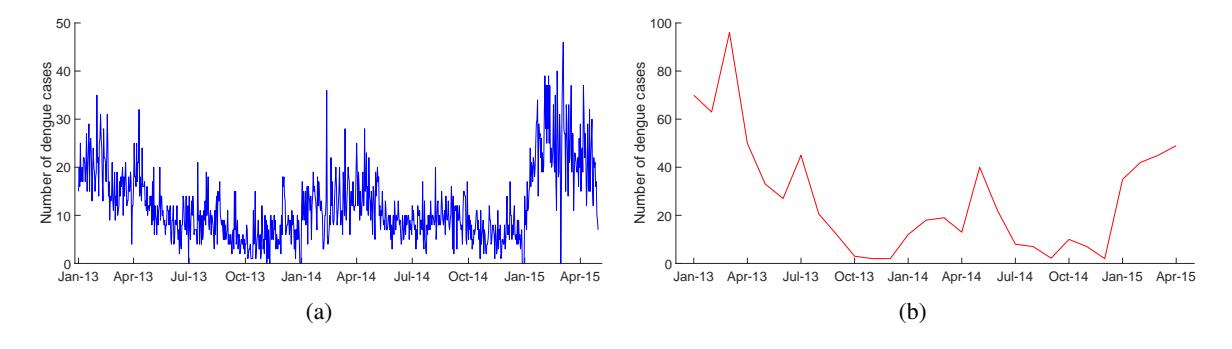
Figure 1: (a) Daily dengue data in Semarang; (b) Monthly dengue data in Malang.
Semarang has the area of 373.67 square kilometers, and the downtown is located 2.45 meters above sea level. The total population of Semarang has approximately \(N_s=1.5\) million people, making it the fifth most populous city in Indonesia. It has many manufacturing and high-tech industrial areas, well known as a massive industrial city. The percentage of the green space is about 7.5 percent of total area [29]. In another hand, Malang has elevation 440-670 meters above sea level with an entire area of 145.28 square kilometers. There are approximately \(N_m=0.9\) million inhabitants. The economic and demographic growth in the last decades transforms the city into an important commercial center. The proportion of land covered with the building is increasing, but agriculture land is still a dominant area. Green space in Malang has a higher percentage than Semarang, closely 18 percent [30].
Semarang and Malang have a high risk of dengue endemic. Health department office notes that big cities in Java potentially become the most significant sources in Indonesia. Dengue data in both cities have different
basis, see Fig. 1. Semarang Health Office has recorded the daily dengue cases (hospitalized) from January 2013 to April 2015. Dengue data in Malang has a monthly basis, collected by Malang Health Office in the same period [9]. There is no separation on data as dengue fever (DF), dengue hemorrhagic fever (DHF), or dengue shock syndrome (DSS), so a total number of dengue cases can be considered as the sum of all levels.
3. MATHEMATICAL MODEL
The basic premise commonly used in construction of a mathematical model for infectious disease is division of the population into some different classes [2], [14]. The susceptible-infected-recovered (SIR) type model is a simple model for some disease transmission, become the most generally used framework for epidemiology. Dengue transmission in host and vector is modeled by SIR-UV type, where the host compartments are labeled SIR classes and the vector compartments are labeled UV classes.
The classical disease transmission model introduced by Kermack and McKendrick (1927) with some modification by Gotz (2017) is adapted to obtain the description of host-vector dengue transmission dynamics.
\[\begin{split} \frac{dS(t)}{dt} &= \mu(N - S(t)) - \frac{\beta}{M} S(t) V(t), \\ \frac{dI(t)}{dt} &= \frac{\beta}{M} S(t) V(t) - (\gamma + \mu) I(t), \\ \frac{dR(t)}{dt} &= \gamma I(t) + \mu R(t), \\ \frac{dU(t)}{dt} &= \alpha - \frac{\delta}{N} U(t) I(t) - \eta U(t), \\ \frac{dV(t)}{dt} &= \frac{\delta}{N} U(t) I(t) - \eta V(t), \end{split}\] \[(1)\] where variable S,I, and R are the susceptible, infected, and recovered human respectively. The total population of human, denoted by N and assumed to be constant. Variable U and V denote susceptible and infected mosquitoes respectively. The parameter \(\beta\) denotes the infection rate of vector to human and \(\delta\) denotes human to vector infection rate. Parameter \(\gamma\) is recovery rate of infected human. The mortality rate of human and mosquito are denoted as \(\mu\) and \(\eta\) respectively. We assume that the population of vector is constant \((U(t) + V(t) = M \in \mathbb{N})\), consequently \(\alpha = \eta M\).
There are some unobserved parameters in the model, such as \(\beta\) and \(\delta\). Therefore, we propose a reduction of host-vector model by using the coexistence equilibrium of mosquitoes [14]. The mosquitoes dynamic is faster compared to the host dynamic as the impact of many mechanisms. Therefore, an option that can be used is considering the mosquito population on dengue transmission model to be in its coexistence equilibrium.
\[U^* = \frac{\nu MN}{I + \nu N}, \qquad V^* = \frac{MI}{I + \nu N},\] where \(\nu = \eta/\delta \approx 1/2\) [14]. By substituting the coexistence equilibrium and S(t) = N - I(t) - R(t), we obtain the reduced model as follows.
\[\frac{dI(t)}{dt} = \beta(N - I(t) - R(t)) \frac{I(t)}{I(t) + \nu N} - (\gamma + \mu)I(t),\] \[\frac{dR(t)}{dt} = \gamma I(t) - \mu R(t).\] (2)
However, to obtain a more realistic description of dengue dynamics in both cities with different human population size, we afterward consider a model based on the number of dengue cases per 100,000 inhabitants. By multiplying every state variables with the constant \(\kappa=100,000/N\), then we have a system as shown in the following equations. Variables \(\overline{I}(t)\) and \(\overline{R}(t)\) respectively denote the number of infected and recovered individuals on \(\overline{N}=100,000\) inhabitants.
\[\frac{d\overline{I}(t)}{dt} = \beta \left( \overline{N} - \overline{I}(t) - \overline{R}(t) \right) \frac{\overline{I}(t)}{\overline{I}(t) + \nu \overline{N}} - (\gamma + \mu) \overline{I}(t),\] \[\frac{d\overline{R}(t)}{dt} = \gamma \overline{I}(t) - \mu \overline{R}(t).\] (3)
The two dimensional dengue model gives two equilibrium points, trivial equilibrium \((\overline{I}, \overline{R}) = (0,0)\) and non-trivial equilibrium:
\[(\overline{I}^*, \overline{R}^*) = \left(\frac{(\mu \overline{N})(\beta - \nu(\mu + \gamma))}{(\beta + \mu)(\gamma + \mu)}, \frac{(\gamma \overline{N})(\beta - \nu(\mu + \gamma))}{(\beta + \mu)(\gamma + \mu)}\right),\] with components of non-trivial equilibrium will have positive value if \(\beta \geq \nu(\mu + \gamma)\). The Jacobian matrix of non-trivial equilibrium is given by J with \(\rho = \gamma/\mu, \varsigma = \beta/\mu\), and \(\phi = \frac{\nu(\rho+1)-\varsigma}{\nu(\rho+1)+1}\).
\[J = \begin{bmatrix} \frac{(1+\rho+\varsigma)\phi}{\varsigma} & \phi \\ \rho & -1 \end{bmatrix}.\]
Hence we get a polynomial characteristic as follows.
\[P(\lambda) = \lambda^2 + \left(1 - \frac{(1 + \rho + \varsigma)\phi}{\varsigma}\right)\lambda - \phi\left(\rho + \frac{1 + \rho + \varsigma}{\varsigma}\right).\]
Non-trivial equilibrium is locally asymptotically stable if the real part of the Jacobian matrix eigenvalues are negative. Based on the Hurwitz criterion, polynomial characteristic with non-negative coefficients ensures that its roots have negative real parts. Therefore the endemic equilibrium will be locally asymptotically stable if these conditions are satisfied.
\[1 - \frac{(1+\rho+\varsigma)\phi}{\varsigma} \ge 0, \qquad -\phi\left(\rho + \frac{1+\rho+\varsigma}{\varsigma}\right) \ge 0.\]
From the second equation, since \(\rho\) and \(\varsigma\) are non-negative then we get \(\phi \leq 0\) that implies \(\beta \geq \nu(\gamma + \mu)\). Therefore the non-trivial equilibrium \((\overline{I}^*, \overline{R}^*)\) becomes locally asymptotically stable if \(\beta \geq \nu(\mu + \gamma)\).
Table 1: Parameter values used in the simulation
| Parameter | Symbol | Value | Unit | References |
|---|---|---|---|---|
| Host mortality rate | \(\mu\) | \(1/(65 \cdot 48)\) | week-1 | [5], [14] |
| Vector mortality rate | \(\eta\) | 7/10 | \(week^{-1}\) | [5], [14] |
| Infection rate of vector to host | \(\beta\) | estimated | week-1 | - |
| Infection rate of host to vector | \(\delta\) | \(2\eta\) | \(week^{-1}\) | [14] |
| Recovery rate | \(\gamma\) | 7/6 | week-1 | [3], [15] |
| Initial proportion of susceptible individuals | \(S_0\) | \(56.9\% \cdot N\) | people | [3], [24] |
| Total population in Semarang | \(N_s\) | \(1.5 \cdot 10^{6}\) | people | - |
| Total population in Malang | \(N_m\) | \(9 \cdot 10^{5}\) | people | - |
For simulation, the parameter of infection rate \(\beta(t)\) is considered to be time-dependent. The remaining parameters, \(\gamma\), \(\mu\), and \(\nu\) are assumed to be constant throughout observation time and their values are obtained from some literature. By using an assumption that each month consists of four weeks, we list the parameter values in Table 1.
4. SPIRAL DYNAMIC OPTIMIZATION
Spiral dynamic optimization is a metaheuristic method constructed by the analogy of the natural phenomena, spiral motion in nature. A metaheuristic is a heuristic approximation framework for continuous or discontinuous optimization problems. Heuristic algorithms are commonly used to solve nonlinear and more complicated optimization problems that make it popular in the computational process [28]. Simple structure, ease of use, quick results, local searching capacity, and few control variables are some advantages of spiral dynamic optimization [27], [28].
The dynamic of spiral path motion is the core characteristics of spiral optimization. A large iteration will be getting a smaller radius when it is close to the optimum point that always becomes the center of spiral shape [27]. Angle and radius of rotation are parameters of spiral optimization. They are already fixed at the beginning and won't change during iteration [27], [28]. Moreover, the radius and angle affect the distance between two points on the trajectory.
This method use rotation matrix to find the optimized infection rate \(\beta\) evaluated based on objective function \(F(t,\beta) = \|I^{data}(t) - I^{model}(t)\|_2\). \(I^{data}(t)\) and \(I^{model}(t)\) denote dengue data and simulation respectively at time t per 100.000 inhabitants. The algorithm of this optimization is shown below.
- 1) Preparation: Generate m random point in feasible region, \(\beta_i(0) \in \mathbb{R}^n, i = 1, 2, 3, ..., m\). Give the value of rotation angle \(\theta\), circle radius r and maximum iteration \(k_{max}\). Set k = 0.
- Initialization: Set \(\beta_i(0), i = 1, 2, 3, ..., m\) as the initial points and set the rotation center \(\beta^*\) as \(\beta^* = \beta_{i_g}(0), i_g = \arg\min_i F(t, \beta_i(0)).\)
- 3) Updating \(\beta_i\): For i = 1, 2, 3, ..., m, update \(\beta_i(k+1) = S_n(r,\theta) \cdot \beta_i(k) (S_n(r,\theta) I_n) \cdot \beta^*(k)\) with \(S_n(r,\theta) = diag(r,r,...,r) \cdot \prod_{i=1}^{n-1} \left(\prod_{j=1}^{i} R_{n-i,n+1-j}^{(n)}\right)\) and entries of matrix \(R_{n-i,n+1-j}^{(n)}\) are defined by: \(r_{ii} = r_{jj} = \cos\theta, r_{ij} = -\sin\theta, r_{ji} = \sin\theta, r_{pq} = 1\) if p = q and \(r_{pq} = 0\) if \(p \neq q\). 4) Updating \(\beta^*\): For i = 1, 2, 3, ..., m, update \(\beta^*(k+1) = \beta_{ig}(k+1), i_g = \arg\min_i F(t, \beta_i(k+1))\)
- but you need to ensure that center of rotation is always on feasible region.
- Terminal Criterion: If \(k = k_{max}\) then stop. Otherwise, set k = k + 1 and return to step 3.
5. CONVERSION OF DENGUE DATA IN SEMARANG AND MALANG
Provided data of dengue cases in both cities have different basis, daily basis for Semarang and monthly basis for Malang. Before making a comparison, we need to convert both data to weekly basis. For Malang, we use spiral dynamics optimization on a reduced model to get weekly infection rate such that the cumulative infected every four weeks close to the monthly data. This process provides 4 data for each month, so we have 112 weekly data from January 2013 to April 2015. For Semarang, we accumulate 7 or 8 days dengue cases depend on the number of days in a month which provides 4 weeks dengue data. Dengue data in Semarang records the first day of dengue patients admitted to the hospital and got a positive diagnose for being infected by dengue virus, so accumulation process won't count infected patient more than once. Since the dengue data has form 48 weeks each year then the value of the parameter in biological model also uses the assumption that one year equals to 48 weeks.
Let \(I^{data}(t)\) denotes the observed dengue cases in month t and \(I^{model}(\tau)\) denotes the infected human (from the reduced model) in week \(\tau\). Since observed data is monthly and the output of the system is weekly basis then output in month t, denoted by \(I_{est}^{model}(t)\) is calculated as an accumulative infected human every four weeks.
\[I_{est}^{model}(t) = \sum_{\tau=4t-3}^{4t} I^{model}(\tau).\]
In one month, we need to find infection rate for each week \(\beta = [\beta_1 \quad \beta_2 \quad \beta_3 \quad \beta_4] \in \mathbb{R}^4\) which is minimizing the objective function \(F(t,\beta) = \|I^{data}(t) - I^{model}_{est}(t)\|_2\). To find the optimized infection rate, \(\beta \in \mathbb{R}^4\), we used the spiral dynamics optimization method with m=1000. We generated it by using a Sobol sequence to get initial random points. Next, we take \(\theta=\pi/4\), r = 0.99, and \(k_{max} = 50\). The accumulative weekly data every month have a good fitting to the monthly data in Malang. See Fig. 2, we give the plot of the weekly basis of infected as a conversion result. There is also the comparison between monthly data and simulation of infected in Malang.
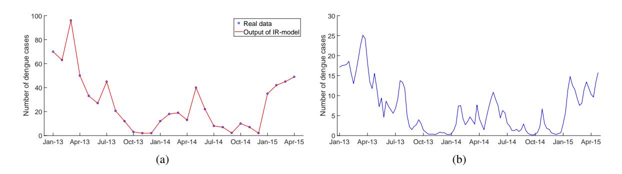
Figure 2: (a) Comparison between data and simulation in monthly basis; (b) Weekly dengue data produced by optimization in Malang.
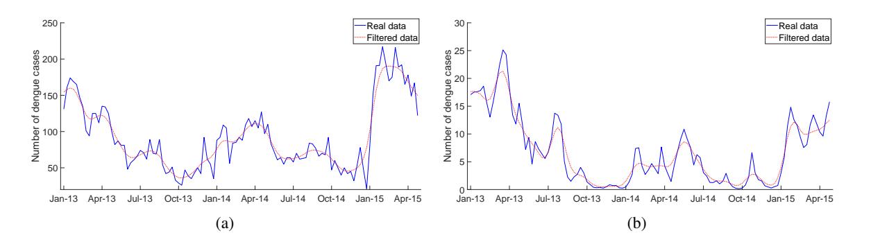
Figure 3: Real data and Gaussian filtered data of dengue cases in (a) Semarang and (b) Malang.
The raw data shows high-frequency fluctuations. Hence, we implement the Gaussian filter to eliminate frequently oscillation to obtain smoothed data. The filter uses the weighted average based on a Gaussian function to removes the randomness of observed data. In Fig. 3, we show the comparison between weekly observed data and filtered data resulted by Gaussian filter in Semarang and Malang.
6. SIMULATION OF FITTING
To describe the pattern of dengue transmission, we treat infection rate \(\beta\) as a time-dependent parameter and its values for each time interval \([t,t+\Delta t]\) are obtained by using spiral dynamic optimization to minimize the error between filtered data and infected. Let \(\beta_*(t)\) is time-dependent infection rate produced from the method. We take \(m=1000, \theta=\pi/4, r=0.99\), and maximum iteration \(k_{max}=50\) for the optimization. Unfortunately, rotation does not work in one-dimensional space, so \(\theta\) does not affect the process. The generated points are just like shrinking or moving closer to a point which is minimizing the objective function. In Fig. 4, we plotted weekly infection rate \(\beta_*(t)\) in both cities and presented mean, variance, minimum, and maximum in Table 2. Fig. 5 shows a comparison between filtered data and infected by using \(\beta_*(t)\) in Semarang and Malang respectively. The output matches qualitatively well with the data as a consequence of minimizing the cost function.
During January 2013 to April 2015, the number of dengue incidence in Semarang is relatively higher than Malang. We can find 6.152 dengue cases per 100,000 inhabitants in Semarang, approximately eight times the amount of incidences in Malang, 0.744 cases. The highest and lowest number of recorded dengue in Semarang are 12.48 in the third week of February 2015 and 2.40 in the second week of October 2013 respectively. Lower cases can be found in Malang with the highest case 2.36 on the third week of March 2013 and the lowest case 0.05 on the first week of November 2013. Many possibilities can lead to differences
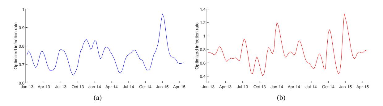
Figure 4: Weekly infection rate \(\beta_*(t)\) in (a) Semarang and (b) Malang.
in dengue spread in both cities. Natural factors and human lifestyle have a strong impact on dengue endemic [18]. Semarang as a lowland area has a relatively warmer temperature, high percentage of humidity, and high cumulative rainfall then Malang as a highland area. Temperature, humidity, and precipitation seemingly correlate with the dengue behavior [6], [20]. Warm temperature, suitable humidity, and intense rainfall are driving force to construct an ideal environment for mosquitos life cycle. The active urban area in Semarang provides a dense concentration of resident forms favorable situations for the prevalence of dengue [20].
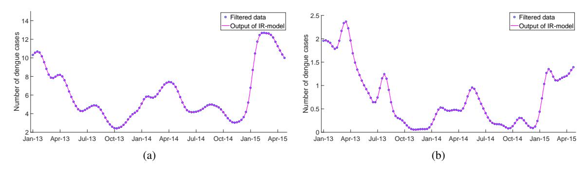
Figure 5: Comparison between filtered data and simulation per 100,000 inhabitants by using \(\beta_*(t)\) in (a) Semarang and (b) Malang.
High dengue incidence in Semarang and Malang occurs in January to April each year from 2013 to 2015, a period with high precipitation in Semarang and Malang. It can be explained that the aquatic environment is the breeding site of mosquitoes. Mosquitoes probably complete their breeding in water containers inside and around residence after rainfall [10]. Areas of stagnant water such as bottles, uncovered barrels, cans, flower vases, discarded tires, and buckets allow the mosquitoes to lay their eggs. Expansion of breeding site during the rainy season triggers the abundance of mosquito population and indirectly affect the spread of dengue virus [6], [12].
Table 2: Statistic data on dengue infection rate \(\beta_*(t)\)
| City | Mean | Variance | Maximum | Minimum |
|---|---|---|---|---|
| Semarang | 0.7468 | 0.0038 | 0.9739 | 0.6417 |
| Malang | 0.7412 | 0.0324 | 1.3329 | 0.4073 |
Based on the mean value of infection rates obtained by spiral dynamic optimization, it can be seen that dengue transmission in Semarang is slightly higher than Malang. The value of variance indicates that the rate of dengue transmission in Malang is more distributed than Semarang. In the period of July 2013 to February 2014 and September 2014 to February 2015, it is shown some significant increasing and decreasing of the value β∗(t) in short time intervals. At the time interval t to t + 4t, the distinct value of I(t) in Semarang and Malang with same 4I = I(t) − I(t + 4t) will produce different value of β∗. The changes 4I with a condition I(t) close to zero will reveal larger change on infection rate β∗ than using a higher value of I(t), and it can be seen clearly in December 2014.
The pattern of the dengue transmission rate β∗ in Semarang shows that the third week of September 2013 and October 2014 become the starting point of increasing β∗(t) until it reaches the peak and persists at a high level in next months. By comparing the pattern of infection rate and the increasing number of infected, there is a backward shift approximately 4-5 weeks where dengue cases begin to crawl up in the third week of October 2013 and fourth week of November 2014. Distinct trends of dengue transmission can be found in Malang. The infection rate begins to increase in the third week of October 2013 and the first week of December 2014. With a backward shift close to 2-3 weeks, dengue incidence starts to grow in the second week of November 2013 and the third week of December 2014.
Furthermore, before the infection rate in Malang increases to its peak, there is an unusual condition such as increasing and decreasing of infection rate in the first week of September to the third week of October 2013 and the first week of October to the third week of November 2014. This problem can be seen in dengue incidence as the reappearance of dengue cases after the almost zeros incident in the previous period, and then the incidence will decrease again like disappeared in the next period. Although the infection rate does not increase significantly, it can be the initial alarm for the occurrence of dengue outbreak. This information is useful in determining the period of the dengue prevention strategy.
Semarang and Malang have different initiation periods when infection rate starts to increase. The end of September to mid-October is starting time for increasing the infection rate in Semarang. In Malang, although a significant increase in the infection rate occurs in December, the period from early September to October should be considered as the beginning of re-emergence of dengue cases. The difference in the initiation period of infection rate Semarang and Malang is close to 2-3 weeks. A distinct period of increasing infection rate influences the initial period of dengue incidence in both cities where Malang is 2-3 weeks faster than Semarang, so the increase of dengue cases that occurred in Malang is also earlier. Meteorological conditions [6] can influence initiation periods of an outbreak in both cities. A different period of starting rainfall in Semarang and Malang may lead to changes in a time when the dengue are beginning to occur [10]. The peaks of dengue incidence occur 2-4 weeks slower than the peaks of the transmission rate in both cities. It is possibly an effect of the different characteristic of the infection, such as the incubation period of virus and response of human immune [13]. Information about the pattern of dengue cases can be used by a public health agency to improve dengue control and surveillance. Period of the outbreak can be a reference of the early warning system and disease prevention program [6], [12]. Since efforts to reduce dengue fever are limited to mosquito population control, traditional efforts such as eradication of mosquito nests and fogging in the right time are substantial methods for dengue prevention.
7. SEASONAL INFECTION RATE OF DENGUE TRANSMISSION MODEL
Seasonal variation in the cases of infectious disease is commonly found in the area characterized both tropical and subtropical climate. The causes of seasonal change and periodicity of infectious diseases have confused epidemiologist [13]. Some different mechanisms trigger a seasonal transmission of infectious diseases such as survival of pathogen outside host [23], [25], host behavior [13], host immune function [12], and plenty of vector [16], [23]. The survival of the parasite organism outside a human and abundance of disease vectors are positively correlated with the characteristics of the environment, especially meteorological variables. The pattern of climate variability can give a response to the annual variety of transmission and impact on seasonal or complex cases. The effect of seasonality is important in dengue transmission, particularly for Aedes mosquito as there is a period in which its population is overload, wet season [17]. In tropics and subtropics areas that receive more precipitation, the spread of dengue is very much dependent on seasonal variations. The peak of infection occurred during the rainy season because there are a lot of water-holding containers. Moreover, seasonality can give an effect on the effectiveness and efficiency of vector control strategies by identifying the appropriate period of starting larvicide and adulticide measure to reduce the mosquito population [31].
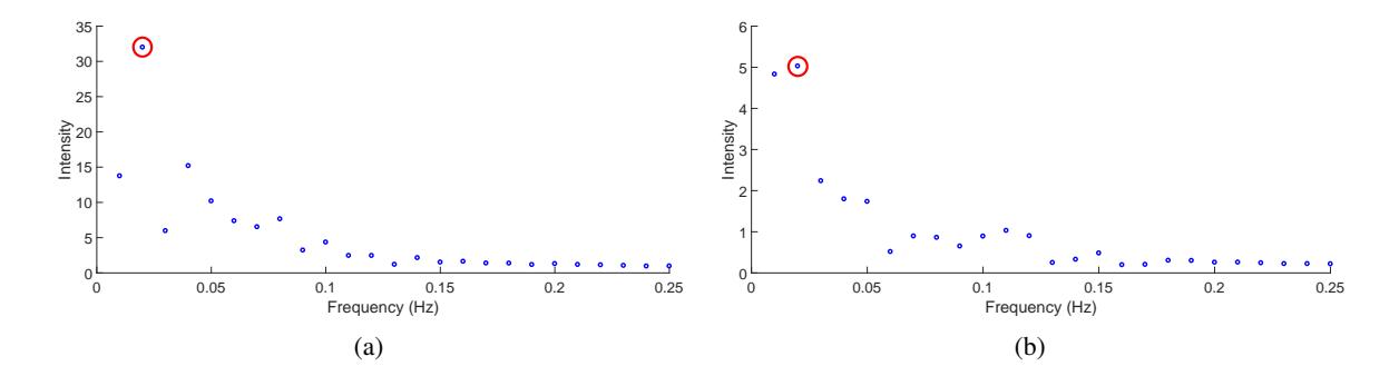
Figure 6: Fourier spectrum of filtered data in (a) Semarang and (b) Malang.
Implementing a fast Fourier transform to filtered data in Semarang and Malang, we obtain a Fourier spectrum shown in Fig. 6. Fourier spectrum exhibits an annual periodicity of the dengue cases. The observed peak relates to a frequency of f=0.02 or equivalently period T=50 weeks nearly resembling an annual pattern.
Seasonality is incorporated in the model via a periodic function of the infection rate, denoted by \(\beta_{\sim}(t)\). This representation is inspired by field observations of the actual vector dynamics which shows seasonal patterns. To input seasonality into the dengue transmission model, the infection rate will be approximated to be a periodic function of time and we use a sinusoidal function [1], [13]:
\[\beta_{\sim}(t) = \beta_0 + \sum_{k=1}^{n} \left[ \eta_k \cdot \cos(k\omega t + \psi_k) + \zeta_k \cdot \sin(k\omega t + \phi_k) \right],\] where \(\beta_0\) is the average transmission rate, \(\omega\) is the period of seasonality, \(\eta_k\) and \(\zeta_k\) are the amplitude, and n is the number of the mod. The simple sinusoidal function is sufficient to obtain a description of the temporal forcing in the dengue incidence as it is driven by seasonal climate cycles, although there are many elaborate functions can be chosen. The value of parameter \(\omega\) is \(2\pi/T\) with T stands for the period of seasonality (usually one year), and the remaining parameter is obtained by optimization. Based on the observation of annual dengue data in Fig. 7, we will use mod n=3 of sinusoidal function and compare between the result with \(\beta_{\sim}(t)\) and actual data in both cities.
In order to find the value of each parameter in sinusoidal function, \(\beta_0, \eta, \zeta, \psi\), and \(\phi\), we use spiral dynamic optimization that minimizing deviation output of model and incidence data. We set \(m=10000, \theta=\pi/4, r=0.99\), and \(k_{max}=1000\). In Table 3, we can see the coefficients of seasonal infection rate in Semarang and Malang
Based on the value of amplitude for each mod of seasonal infection rate, Semarang and Malang have a different dominant mod of wave. Dominant mod in Semarang is n=2; it means that the wave has similar behavior each half of a year. Malang has dominant mod n=3, so the pattern of infection rate is almost the same for every four months. The maximum amplitude of cosine and sine reveal that the infection rate in Malang is more varied than Semarang. Non-zero center of amplitude \(\beta_0\) shows that infection in Semarang is higher than Malang.
In Fig. 8, we compile the results of the model with input seasonal infection rate in Semarang and Malang. It is shown the comparison between the simulation results for the infection rate and observed dengue cases. The annual pattern is well produced, but the output in some period is less match with the data. The fluctuation of incidence is frequently observed, there is a decline in the susceptible individuals during an epidemic period caused by partially protective immunity. Low incidence follows on next period while the susceptible population is replenished until an outbreak is possible to occur again [13]. The seasonal infection rate in Semarang and Malang are given by in Fig. 9.
The seasonal infection rate with a sinusoidal function will produce a periodic output every year with some magnitudes. The annual pattern in Semarang is created well, but there are some mismatches in some periods.
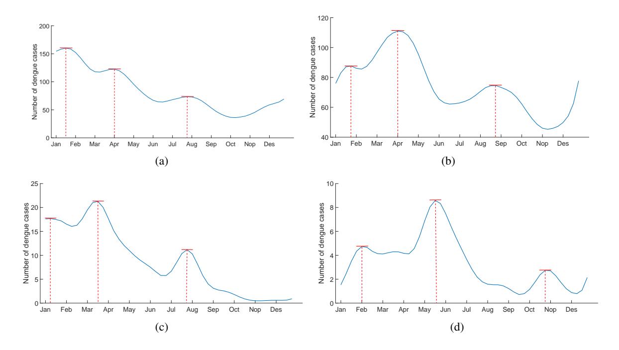
Figure 7: Number of mod in annual dengue cases from Semarang in (a) 2013; (b) 2014 and Malang in (c) 2013; (d) 2014.
Table 3: Parameters value of seasonal infection rate \(\beta_{\sim}(t)\).
| Parameter | Definition | Semarang | Malang |
|---|---|---|---|
| \(\beta_0\) | non-zero center amplitude | 0.75726 | 0.75543 |
| \(\eta_1\) | cosine amplitude for mod 1 | -0.06031 | 0.10471 |
| \(\eta_2\) | cosine amplitude for mod 2 | -0.46831 | 0.27553 |
| \(\eta_3\) | cosine amplitude for mod 3 | -0.05788 | 1.14654 |
| \(\zeta_1\) | sine amplitude for mod 1 | -0.01076 | -0.20158 |
| \(\zeta_2\) | sine amplitude for mod 2 | 0.43518 | 0.36945 |
| \(\zeta_3\) | sine amplitude for mod 3 | -0.08099 | 1.01626 |
| \(\psi_1\) | cosine phase for mod 1 | 3.59831 | 4.35402 |
| \(\psi_2\) | cosine phase for mod 2 | -3.55353 | 4.53131 |
| \(\psi_3\) | cosine phase for mod 3 | -6.49679 | 8.11560 |
| \(\phi_1\) | sine phase for mod 1 | 9.96002 | -7.23474 |
| \(\phi_2\) | sine phase for mod 2 | 4.18387 | -3.50418 |
| \(\phi_3\) | sine phase for mod 3 | 5.60604 | 6.47901 |
Apparent differences between the simulation and data occur in January 2014. This condition can be explained that the sinusoidal function used for simulation in Semarang reveals the peak of dengue cases in January and is not fulfilled at these two periods. With the initial time in October 2013, dengue cases increase until the beginning of 2014 and reach a peak in April. The second mismatch shows that the output produces a peak of incidence about 3-4 weeks earlier. A good approximation is also demonstrated by the results of the fitting model with seasonal infection rates and data throughout 2013 in Malang. Mismatches emerge in mid-2014 and early 2015. Simulations do not indicate a high frequency of dengue cases in mid-2014, but data shows
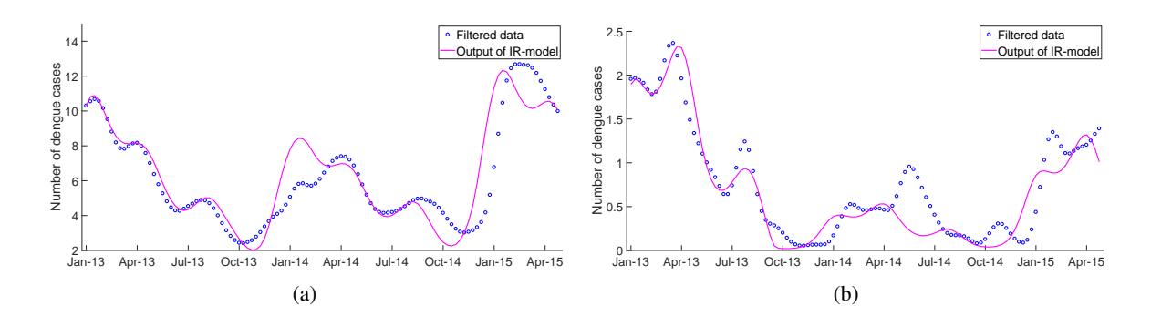
Figure 8: Comparison between filtered data and simulation per 100,000 inhabitants by using seasonal infection rate in (a) Semarang and (b) Malang.
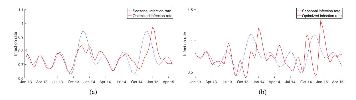
Figure 9: Seasonal infection rate in (a) Semarang and (b) Malang.
that May is the peak of dengue outbreak. Similar to Semarang, the output of the model at the end of 2014 is shifted 3-4 weeks earlier than data. The seasonal infection rate in Malang shows the peak of dengue cases occurs at the end of March in 2013 and 2015.
In Fig. 9, the comparison between the infection rate resulted by optimization and the seasonal infection rate in Semarang shows similar characteristics throughout 2013 until mid-2014. The period that becomes the initial of increasing infection rate occurs at the end of September every year. This condition was suitable in 2013, but there is a mismatch in 2014 due to the shifting of the point that becomes the initial increasing rate. Messy behavior of transmission rate in Malang causes seasonal infection rate producing a good approximation only in the first nine months of 2013 and an unfortunate result in the next period. The starting point of increasing infection rate is indicated 2-3 weeks earlier than Semarang, early September, and this condition is suitable with the starting point resulted by optimization. The period of dengue cases arises, disappears, and re-emerges at a higher level does not appear in the infection rate, but the top level is revealed.
8. CORRELATION BETWEEN DENGUE AND CLIMATE FACTOR
Changes in weather and climate conditions can influence the Aedes mosquitoes through complex and multiple mechanisms. Temperature is an essential determinant of vector biting rate, development of the egg and immature mosquito, breeding time of virus in the mosquito (extrinsic incubation period), and survival at each stage of mosquito life cycle [10], [12]. Rainfall expands habitat for the aquatic stages of the mosquito development and strongly affects the distribution of vector [14]. The effects of rainfall and evaporation on available water sources can regulate the population, size, and behavior of Aedes mosquitoes. Humidity gives effects on mosquito competence, intensity of biting activity, and adult mosquito lifespan [10].
The recent study of Center of Climate Change and Air Quality Indonesian Agency for Meteorology, Climatology, and Geophysics (BMKG) reveals that the most correlated meteorological data with incidence
case is humidity [4]. Eighty percent of severe dengue cases over the period of January 2013 to April 2015 occurs when humidity is more than 75 percent [10]. Higher probability of ideal humidity will emphasize the opportunity of increasing vector population and automatically affects the possibility of an outbreak. Pearson correlation test of humidity, optimized infection rate, and dengue incidence in Semarang and Malang is shown in Table 4. In general, the value of Pearson correlation on Semarang data shows more positive linear correlations between incidence, transmission rate, and humidity as a meteorological factor.
| City | Aspect | Humidity | Infection rate | |
|---|---|---|---|---|
| Semarang | Infection rate | correlation: 0.385 | - | |
| p-value: ≤ 0.05 | - | |||
| Dengue Incidence | correlation: 0.516 | correlation: 0.061 | ||
| p-value: ≤ 0.05 | p-value: 0.521 | |||
| Malang | Infection rate | correlation: 0.182 | - | |
| p-value: 0.054 | - | |||
| Dengue Incidence | correlation: 0.370 | correlation: 0.054 | ||
| p-value: ≤ 0.05 | p-value: 0.575 | |||
Table 4: Pearson correlation of humidity, optimized infection rate, and dengue incidence.
Fig. 10 shows cross-correlation analysis with time-lag. Semarang and Malang have almost the same lag between humidity, infection rate, and dengue incidence. A lag between humidity and dengue incidence in Semarang is five weeks, and Malang has two weeks longer than Semarang, which is lag seven weeks of humidity and incidence. A lag between humidity and infection rate is shorter than incidence, consecutively one and three weeks for Semarang and Malang. The lag between humidity and infection can be understood that it needs several days after the favorable weather conditions to create the ideal habitat for mosquito development and drive an abundance of vector population that can increase the possibility of dengue infection. The lag between infection and incidence can be explained as the impact of the intrinsic incubation period of virus inside human body after biting and the reaction of antibody to the dengue virus [6]. Therefore, not at the day where the ideal humidity is achieved then the high infection occurs and not at the day where high infection produces its peak directly, but it needs several periods between each process. The lag time between weather, infection, and outbreaks can be accounted for by the influence of weather conditions on the biological process of the mosquito breeding above. [6], [13].
The difference of time-lag effect on dengue incidence in both cities is possible to occur and had been supported by the fact that several cities in the world have different time-lag between climate variable and dengue outbreaks. Hsieh and Chen indicate that the strongest correlation between dengue outbreaks and humidity in Taiwan at a lag of 8 weeks [6]. Sharmin demonstrates a similar result in Dhaka that dengue incidence is positively associated with climate factor in the previous two months [26]. In Barbados, the small Caribbean island, it is reported distinct lag periods with the highest correlation between humidity and dengue incidence at lag seven weeks [6]. However, in Guangzhou, Sang examine the shorter lag time 4 weeks between dengue outbreak and relative humidity [25].
In Fig. 11, we compile humidity condition together with the number of dengue cases and infection rate resulted by optimization in both cities. The vertical blue line denotes humidity less than 75 percent; otherwise, we use the vertical red line. In Semarang, there is an obvious gap between period with the low percentage of humidity and period of low dengue cases. Humidity and infection rate has a gap of less than one month, shorter than the gap between humidity and incidence. It can be explained that infection occurs between favorable humidity and dengue outbreaks. The gap between the period of suitable humidity condition and incidence in Malang seems vague, but it is a little longer than the gap in Semarang. The unusual ccondition, rapid change of infection rate in a short time, occurs during the period with a low percentage of humidity.
Finally, The causes of the different lag period between weather condition and dengue incidence in some cities can not precisely be described. Natural background and social activity are two of the primary mechanisms that drive the distinction of the time-lag effect on dengue cases.
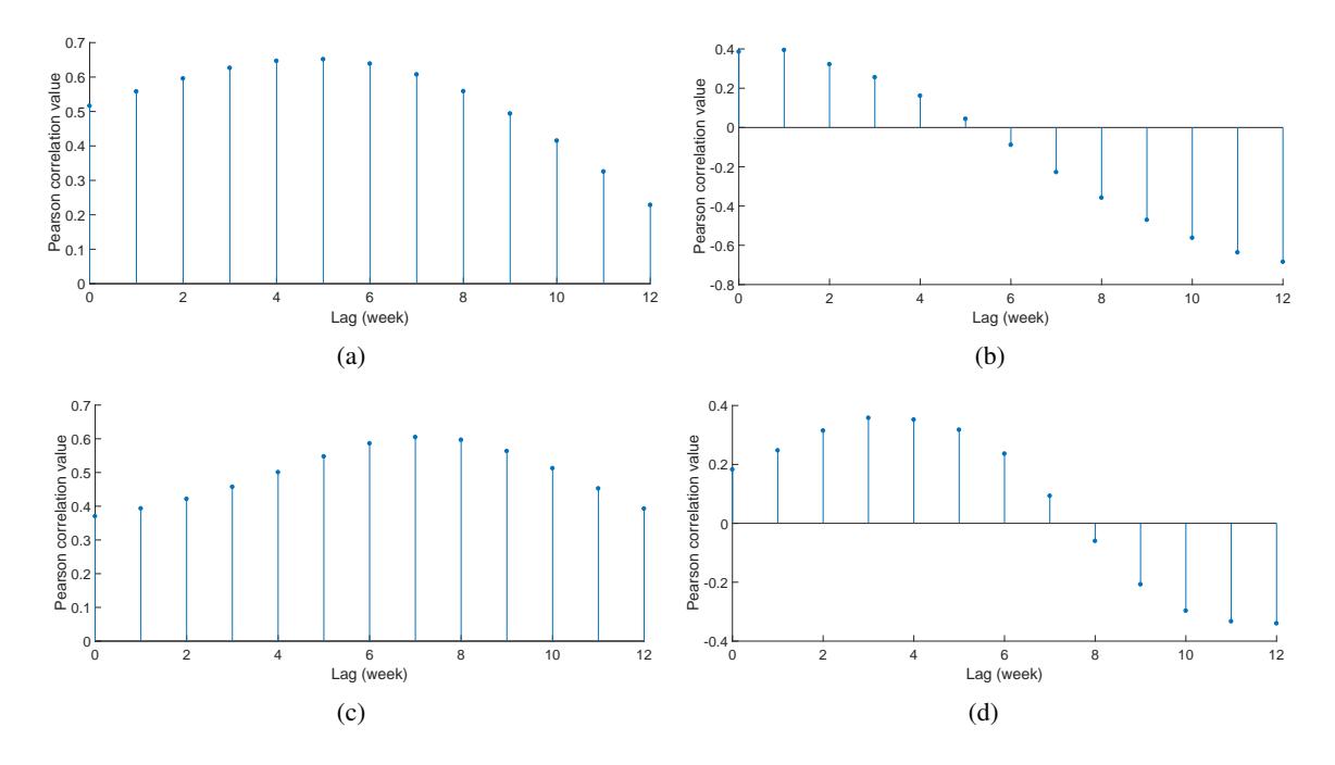
Figure 10: Pearson's linear correlation between (a) Dengue cases and humidity in Semarang; (b) Infection rate and humidity in Semarang; (c) Dengue cases and humidity in Malang; (d) Infection rate and humidity in Malang.
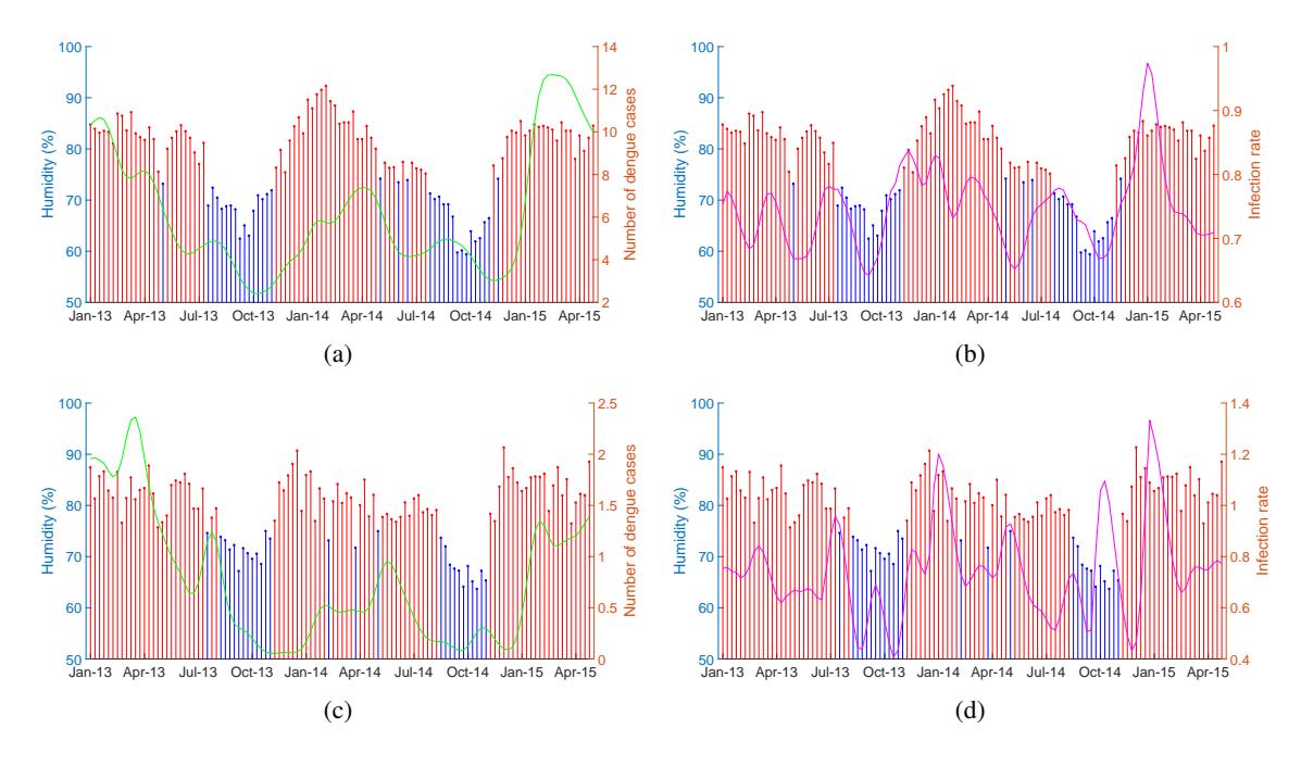
Figure 11: Plot of (a) Humidity and dengue cases in Semarang; (b) Humidity and infection rate in Semarang; (c) Humidity and dengue cases in Malang; (d) Humidity and infection rate in Malang.
9. CONCLUSION
Our primary concern in this paper is to estimate the infection rate parameters and compare dengue transmission in two cities with different background. Therefore, a reduced model describing dengue transmission dynamic is adapted from an existing model. We reduced vector compartment in its coexistence equilibrium since there is no reliable data. We consider infection rate β as the time-dependent parameter and determine it based on the data while the other parameters are assumed to be constant. Spiral dynamic optimization is applied to find the weekly infection rate using the model. The infection rate reproduces good approximation with the actual data in both cities.
Different environmental characteristic and social activity will reveal the different effect of dengue infection rate. Infection rate resulted by optimization method shows that Semarang is slightly higher than Malang. Highest dengue cases in both cities occur in January to April every year that possibly caused by the abundance of the vector on rainy season. The two cities have different take-off periods of dengue, Semarang on last week of September and Malang on the first week of September. Environmental characteristic and human behavior can influence the period of increasing infection and automatically affect the period of increasing incidence. Peaks in dengue cases occur at different period of the years, around 2-4 weeks. A better understanding of seasonal variation in infectious disease, persistence, and periods of dengue outbreak will give more information on determining the efficient control strategies and effective policies.
In the other hand, we have identified seasonal variations of dengue in both cities. Oscillation in dengue incidence is frequently observed and correlated to the oscillation of infection rate. Fourier spectrum exhibits strictly annual pattern with period 50 weeks. Seasonality is incorporated into the model via a Fourier function in the infection rate. This representation is based on actual mosquito dynamics, which is mostly influenced by environmental characteristics. Infection rate potentially high at times of abundance vector population and climatic variables strongly influenced vector population. Furthermore, we also examine the correlation between humidity, infection rate, and dengue incidence. Humidity occurs 1-3 weeks before infection and infection occurs 4 weeks before outbreaks. It can be understood that appropriate weather conditions will increase the mosquito population in the next days. There is an immune effect after bitting inside the human body. However, more detailed analysis of the correlation between dengue cases and climatic data. Not only humidity but also precipitation and temperature will be a challenge for future research.
Although the reduced model and optimization method are able to give a good result for data fitting, the model can be developed more and increased accuracy. Dengue data in Malang can be updated with weekly data rather than using data resulted by conversion of monthly data. By adding the number of mod in sinusoidal function, we will get a better result for infection rate. Humidity is a climate variable that has a significant correlation with dengue incidence and infection rate, but dengue cases in other area are possible to be higher correlated with different climate factors.
ACKNOWLEDGEMENTS
This research was supported by Indonesian Ministry of Education and Culture (Kemdikbud) through BU program for the first author and partially supported by Indonesian Ministry of Research, Technology and Higher Education (Ristekdikti) [grant no. 1511/E4.4/2015] through PMDSU program for the second author.