

1. INTRODUCTION
Mycobacterium Bovis (M. Bovis) is a bacterium that causes zoonotic disease specifically Bovine Tuberculosis (BTB). M. Bovis has a wide range of prospective infected hosts such as cattle and human beings [1]. BTB in cattle initially attacks the lymph which then spread to the lungs. In addition, BTB can also attack the mammae tissue which causes the cattle with BTB disease can also transmit M. Bovis to younger cattle through breastfed [2]. Transmission of BTB in cattle majority occurs through the air. Transmission from animals to humans happens because unfermented milk or undercooked meat. BTB can also be transmitted to humans by air if there is direct contact with BTB infected animals [3].
Bovine Tuberculosis in humans may develop reinfection and relapse same as TB in general. Reinfection occurs when individuals who have had BTB disease are depleted of their immune period and decreased their body defenses. While relapse usually occurs when individuals with BTB not completing the medication prescribed by the doctor or taking wrong medications. The possibility of relapse is between 2-6% for the BTB case [4].
Development in applied mathematics such as mathematical models can be used to control the spread of existing diseases like BTB. For example, author in [5] discusses the optimal control over TB and MDR-TB handling. Furthermore Florian M. etc. [6] discusses about TB disease in humans with reinfection and relapse. Research that discusses the BTB also varied to solve the problem of BTB. As an example Hassan A. S., Garba S. M. and Gumel A. B [7] which discusses the spread of TB in human and animal populations caused by two different bacteria. In addition, De Vos V., Bengis R. G. and Kriek N. [9] discussed the spread of BTB in buffalo population.
In this paper, we will discuss BTB disease in human and cattle population. The model used is based on the deterministic model on [8] which discussed about the spread of BTB in the human and cattle population in Morocco. In this article we add reinfection process and relapse in the human population caused by Myvobacterium Bovis based on [10,11] and also separating human population into two big population, based on their probability to contact with cattle population. The layout of the article is the following: In section 2, the model construction will be discussed and followed with mathematical analysis in section 3. Some numerical simulations based on the basic reproduction number is given in section 4. Some conclusions is given in section 5.
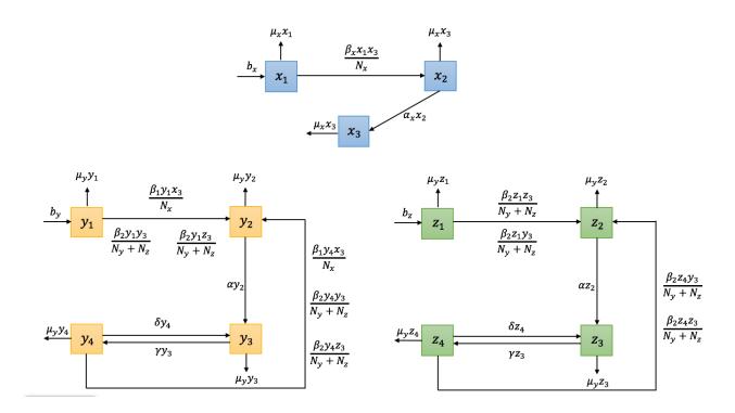
Figure 1: Transmission diagram of BTB model in system 1.
2. MATHEMATICAL MODEL CONSTRUCTION
The idea of the model is to divide the human population into type compartments \((y_i)\) and \((z_i)\), which have and have not direct contact with cattle, respectively. The index i=1,2,3,4 denote the susceptible, exposed, infectious, and recovered having immunity status. On the other hand, cattle population only divided into susceptible \((x_1)\), exposed \((x_2)\) and infectious \((x_3)\) compartment. Here there is no recovered compartment due to the relatively short life time of cattle before they are sent to the market. The transmission diagram of the Bovine tuberculosis is given in Figure 1.
Based on the transmission diagram in Figure 1, the mathematical model which describe the spread of BTB among human and cattle population is given by :
\[\frac{dx_1}{dt} = b_x - \frac{\beta_x x_1 x_3}{N_x} - \mu_x x_1 \tag{1a}\]
\[\frac{dx_2}{dt} = \frac{\beta_x x_1 x_3}{N_x} - \alpha_x x_2 - \mu_x x_2 \tag{1b}\]
\[\frac{dx_3}{dt} = \alpha_x x_2 - \mu_x x_3 \tag{1c}\]
\[\frac{dy_1}{dt} = b_y - \frac{\beta_1 y_1 x_3}{N_x} - \frac{\beta_2 y_1 y_3}{N_y + N_z} - \frac{\beta_2 y_1 z_3}{N_y + N_z} - \mu_y y_1 \tag{1d}\]
\[\frac{dy_2}{dt} = \frac{\beta_1 y_1 x_3}{N_x} + \frac{\beta_2 y_1 y_3}{N_y + N_z} + \frac{\beta_2 y_1 z_3}{N_y + N_z} + \frac{\beta_1 y_4 x_3}{N_x} + \frac{\beta_2 y_4 y_3}{N_y + N_z} + \frac{\beta_2 y_4 z_3}{N_y + N_z} - \alpha y_2 - \mu_y y_2\] (1e)
\[\frac{dy_3}{dt} = \alpha y_2 + \delta y_4 - \gamma y_3 - \mu_y y_3 \tag{1f}\]
\[\frac{dy_4}{dt} = \gamma y_3 - \delta y_4 - \frac{\beta_1 y_4 x_3}{N_x} - \frac{\beta_2 y_4 y_3}{N_y + N_z} - \frac{\beta_2 y_4 z_3}{N_y + N_z} - \mu_y y_4 \tag{1g}\]
\[\frac{dz_1}{dt} = b_z - \frac{\beta_2 z_1 z_3}{N_y + N_z} - \frac{\beta_2 z_1 y_3}{N_y + N_z} - \mu_y z_1 \tag{1h}\]
\[\frac{dz_2}{dt} = \frac{\beta_2 z_1 z_3}{N_y + N_z} + \frac{\beta_2 z_1 y_3}{N_y + N_z} + \frac{\beta_2 z_4 z_3}{N_y + N_z} + \frac{\beta_2 z_4 y_3}{N_y + N_z} - \alpha z_2 - \mu_y z_2 \tag{1i}\]
\[\frac{dz_3}{dt} = \alpha z_2 + \delta z_4 - \gamma z_3 - \mu_y z_3 \tag{1j}\]
\[\frac{dz_4}{dt} = \gamma z_3 - \delta z_4 - \frac{\beta_2 z_4 z_3}{N_u + N_z} - \frac{\beta_2 z_4 y_3}{N_u + N_z} - \mu_y z_4,\tag{1k}\]
supplemented with initial conditions \(x_i(t=0) = x_{io}\) for i=1,2,3 and \(y_i(t=0) = y_{i0}\), \(z_i(t=0) = z_{i0}\) for i=1,2,3,4 are given and positive.
Please note that the total of cattle population is given by:
\[\frac{dN_x}{dt} = \frac{dx_1}{dt} + \frac{dx_2}{dt} + \frac{dx_3}{dt} = b_x - \mu_x(x_1 + x_2 + x_3) = b_x - \mu_x N_x. \tag{2}\]
This is means that number of cattle of population is only depending on birth and natural death rate. Similarly, for human population we have:
\[\frac{dN_y}{dt} = \frac{dy_1}{dt} + \frac{dy_2}{dt} + \frac{dy_3}{dt} + \frac{dy_4}{dt} = b_y - \mu_y(y_1 + y_2 + y_3 + y_4) = b_y - \mu_y N_y, \tag{3}\] and
\[\frac{dN_z}{dt} = \frac{dz_1}{dt} + \frac{dz_2}{dt} + \frac{dz_3}{dt} + \frac{dz_4}{dt} = b_z - \mu_y(z_1 + z_2 + z_3 + z_4) = b_z - \mu_y N_z, \tag{4}\] which also tells us that total of human populations are only depend on birth and natural death rate
In the next section, mathematical analysis regarding the existence and local stability of equilibrium points together with the basic reproduction number will be discussed.
3. MATHEMATICAL ANALYSIS
Since we have the cattle and human population are constant whenever \(b_x=\mu_xN_x\), \(b_y=\mu_yN_y\) and \(b_z=\mu_yN_z\), assuming \(\bar{x}_i=\frac{x_i}{N_x},\ \bar{y}_j=\frac{y_j}{N_y},\ \bar{z}_j=\frac{z_j}{N_z}\), for i=1,2,3 and j=1,2,3,4, we scaled BTB model in equation 1 into:
\[\frac{d\bar{x}_1}{dt} = \mu_x - b_x \bar{x}_1 \bar{x}_3 - \mu_x \bar{x}_1 \tag{5a}\]
\[\frac{d\bar{x}_2}{dt} = b_x \bar{x}_1 \bar{x}_3 - \alpha_x \bar{x}_2 - \mu_x \bar{x}_2 \tag{5b}\]
\[\frac{d\bar{x}_3}{dt} = \alpha_x \bar{x}_2 - \mu_x \bar{x}_3 \tag{5c}\]
\[\frac{d\bar{y}_1}{dt} = \mu_y - b_1 \bar{y}_1 \bar{x}_3 - b_2 \bar{y}_1 \left[ (1 - \rho) \bar{y}_3 + \rho \bar{z}_3 \right] - \mu_y \bar{y}_1 \tag{5d}\]
\[\frac{d\bar{y}_2}{dt} = b_1\bar{y}_1\bar{x}_3 + b_2\bar{y}_1\left[ (1-\rho)\bar{y}_3 + \rho\bar{z}_3 \right] + b_1\bar{y}_4\bar{x}_3 + b_2\bar{y}_4\left[ (1-\rho)\bar{y}_3 + \rho\bar{z}_3 \right] - \alpha\bar{y}_2 - \mu_y\bar{y}_2 \tag{5e}\]
\[\frac{d\bar{y}_3}{dt} = \alpha \bar{y}_2 + \delta \bar{y}_4 - \gamma \bar{y}_3 - \mu_y \bar{y}_3 \tag{5f}\]
\[\frac{d\bar{y}_4}{dt} = \gamma \bar{y}_3 - \delta \bar{y}_4 - b_1 \bar{y}_4 \bar{x}_3 - b_2 \bar{y}_4 \left[ (1 - \rho) \bar{y}_3 + \rho \bar{z}_3 \right] - \mu_y \bar{y}_4 \tag{5g}\]
\[\frac{d\bar{z}_1}{dt} = \mu_y - b_2 \bar{z}_1 \left[ \rho \bar{z}_3 + (1 - \rho) \bar{y}_3 \right] - \mu_y \bar{z}_1 \tag{5h}\]
\[\frac{d\bar{z}_2}{dt} = b_2 \bar{z}_1 \left[ \rho \bar{z}_3 + (1 - \rho) \bar{y}_3 \right] + b_2 \bar{z}_4 \left[ \rho \bar{z}_3 + (1 - \rho) \bar{y}_3 \right] - \alpha \bar{z}_2 - \mu_y \bar{z}_2\] (5i)
\[\frac{d\bar{z}_{3}}{dt} = \alpha \bar{z}_{2} + \delta \bar{z}_{4} - \gamma \bar{z}_{3} - \mu_{y} \bar{z}_{3} \frac{d\bar{z}_{4}}{dt} = \gamma \bar{z}_{3} - \delta \bar{z}_{4} - b_{2} \bar{z}_{4} \left[ \rho \bar{z}_{3} + (1 - \rho) \bar{y}_{3} \right] - \mu_{y} \bar{z}_{4},\] (5j)
\[\frac{d\bar{z}_4}{dt} = \gamma \bar{z}_3 - \delta \bar{z}_4 - b_2 \bar{z}_4 \left[ \rho \bar{z}_3 + (1 - \rho) \bar{y}_3 \right] - \mu_y \bar{z}_4,\tag{5k}\] where \(b_x=\beta_x, b_1=\beta_{h1}, b_2=\beta_{h2}, N=N_y+N_z\) and \(\rho=\frac{N_y}{N}\). Later in the rest of this article, for the sake of written simplification, we rewrite \(\bar{x}_i\) as \(x_i\) again, and also for \(\bar{y}_i\) and \(\bar{z}_i\).
It is easy to prove that for all non-negative initial condition for \(x_i, y_j\) and \(z_j\), then the solutions of the model 5 are non-negative for all \(t \ge 0\) and bounded in the following region.
\[\Phi = \left\{ (x_1, x_2, x_3, y_1, y_2, y_3, y_4, z_1, z_2, z_3, z_4) \in \mathbb{R}_+^{11} : 0 \le x_i \le 1, 0 \le y_j \le 1, 0 \le z_j \le 1 \right\}, \tag{6}\] for i = 1, 2, 3 and j = 1, 2, 3, 4.
Our first analysis is to determine the equilibrium points and their local stability criteria. Before we analyze the model in their complete form, please note that the transmission process in the cattle population is closed to their own population, since infection in cattle population occur only from direct contact between cattle. Therefore, if the BTB initially coming from cattle population in time t=0, then the existence of BTB in human population are also depending on the endemic of BTB in cattle. But instead, the endemic of BTB in cattle do not depend on the endemic of BTB in human population.
There are two equilibrium point in cattle population, i.e the disease free equilibrium \((\omega_1)\) which given by
\[\omega_1 = (x_1, x_2, x_3) = (1, 0, 0), \tag{7}\] and the endemic equilibrium point \((\omega_2)\) which given by
\[\omega_2 = (x_1, x_2, x_3) = \left(\frac{\mu_x \left(\alpha_x + \mu_x\right)}{\alpha_x b_x}, \frac{\mu_x^2 \left(\mathcal{R}_x - 1\right)}{b_x \alpha_x}, \frac{\mu_x \left(\mathcal{R}_x - 1\right)}{b_x}\right),\tag{8}\] where \(\mathcal{R}_x = \frac{\alpha_x b_x}{\mu_x(\mu_x + \alpha_x)}\). It can be seen that \(\omega_1\) always has a biological interpretation for all parameters, while \(\omega_2 \in \mathbb{R}^3_+\) where \(\mathcal{R}_x > 1\). Next, we analyze the local stability criteria of \(\omega_1\) and \(\omega_2\) using their Jacobian matrix. The Jacobian matrix of the cattle sub-population evaluated in \(\omega_1\) is given by
\[\mathcal{J}_{\omega_1} = \begin{bmatrix} -\mu_x & 0 & -b_x \\ 0 & -\alpha_x - \mu_x & b_x \\ 0 & \alpha_x & -\mu_x \end{bmatrix},\] with the characteristic polynomial for the eigenvalue is
\[f(\omega_1) = (\lambda + \mu_x) \left( \lambda^2 + (\alpha_x + 2\mu_x)\lambda + (1 - \mathcal{R}_x)\mu_x(\alpha_x + \mu_x) \right).\]
It is easy to see that \(\omega_1\) is locally asymptotically stable when \(\mathcal{R}_x < 1\).
Similarly, the local stability of \(\omega_2\) also analyzed with the Jacobian matrix approach. The Jacobian matrix of \(\omega_2\) is
\[\mathcal{J}_{\omega_2} = \begin{bmatrix} -\frac{\alpha_x b_x - \alpha_x \mu_x - \mu_x^2}{\alpha_x + \mu_x} - \mu_x & 0 & -\frac{\mu_x (\alpha_x + \mu_x)}{\alpha_x} \\ \frac{\alpha_x b_x - \alpha_x \mu_x - \mu_x^2}{\alpha_x + \mu_x} & -\alpha_x - \mu_x & \frac{\mu_x (\alpha_x + \mu_x)}{\alpha_x} \\ 0 & \alpha_x & -\mu_x \end{bmatrix}.\]
The characteristic polynomial for the eigenvalues of \(\mathcal{J}_{\omega_2}\) is given by
\[f(\omega_2) = \sum_{k=0}^{3} a_k \lambda^k,\] where \(a_0 = \mathcal{R}_x - 1\), \(a_1 = \alpha_x b_x (\alpha_x + 2\mu_x)\), \(a_2 = \alpha_x (\alpha_x + b_x + 3\mu_x) + 2\mu_x^2\), and \(a_3 = \alpha_x + \mu_x\). Based on the Routh-Hurwitz stability criteria, we have that \(\omega_2\) is locally asymptotically stable if \(\mathcal{R}_x > 1\). These result is written in the following theorem.
Theorem 3.1. The cattle population in system 5 has a disease free equilibrium \(\omega_1 = (1,0,0)\) and locally asymptotically stable if \(\mathcal{R}_x < 1\). In the other hand, the endemic equilibrium \(\omega_2 = \left(\frac{\alpha_x(\alpha_x + \mu_x)}{\alpha_x b_x}, \frac{\mu_x^2(\mathcal{R}_x - 1)}{b_x}, \frac{\mu_x(\mathcal{R}_x - 1)}{b_x}\right)\) is exist and locally asymptotically stable if \(\mathcal{R}_x > 1\).
Next we analyze the equilibrium point of the complete model 5. Please note that the BTB can spread among human population because of direct contact between human or with cattle. Therefore, if the BTB already exist in t=0, then BTB might still occur in human population for \(t\to\infty\) even though it already extinct in the cattle population.
The disease free equilibrium of BTB model (5) is given by
\[\Omega_1 = (x_1, x_2, x_3, y_1, y_2, y_3, y_4, z_1, z_2, z_3, z_4) = (1, 0, 0, 1, 0, 0, 0, 1, 0, 0, 0).\] \[(9)\]
Similar with previous way, we analyze the local stability criteria of \(\Omega_1\) using the Jacobian matrix. There are 6 negative eigenvalues, while the other five eigenvalues is given by
\[\mathcal{F}(\Omega_1) = \left(\sum_{k=0}^3 c_k \lambda^k\right) \left(\sum_{k=0}^2 d_k \lambda^k\right),\tag{10}\] where \(c_0=(1-\mathcal{R}_y)\,\mu_y(\mu_y+\alpha)(\gamma+\delta+\mu_y), c_1=(\mathcal{R}_2-1)\left[\alpha(\gamma+\delta)+2\mu_y(\alpha+\delta+\gamma)+3\mu_y^2\right], c_2=\alpha+\delta+\gamma+3\mu_y, c_3=1, d_0=(1-\mathcal{R}_x)\,\mu_x(\alpha_x+\mu_x), d_1=\alpha_x+2\mu_x \text{ and } d_2=1, \text{ where } \mathcal{R}_y=\frac{\alpha b_2(\delta+\mu_y)}{\mu_y(\alpha+\mu_y)(\gamma+\delta+\mu_y)}, \mathcal{R}_2=\frac{\alpha b_2}{\alpha(\gamma+\delta)+2\mu_y(\alpha+\delta+\gamma)+3\mu_y^2}, \text{ and it always hold that } \mathcal{R}_2<\mathcal{R}_y.\) According to Routh-Hurwitz criteria, we have that the \(\text{[rumus tidak dapat ditampilkan dengan baik — lihat PDF asli]}\)have that the \(\Omega_1\) is locally asymptotically stable if \(\mathcal{R}_x < 1\), and \(\mathcal{R}_y < 1\). These results, stated in the following
Theorem 3.2. BTB model in system (5) has a disease-free equilibrium \(\Omega_1\) and locally asymptotically stable if \(\mathcal{R}_x < 1\), and \(\mathcal{R}_y < 1\).
3.1. Basic reproduction number \(\mathcal{R}_0\)
Basic reproduction number define as expected number of secondary cases caused by one primary case during one infection period in a completely susceptible population [20]. Using the next generation matrix approach [21], BTB model in system 5 has the basic reproduction number given by
\[\mathcal{R}_0 = \max \left\{ \mathcal{R}_{0x}, \mathcal{R}_{0y} \right\},\tag{11}\] where \(\mathcal{R}_{0x} = \frac{\alpha_x b_x}{\mu_x (\mu_x + \alpha_x)}\), \(\mathcal{R}_{0y} = \frac{\alpha b_2 (\delta + \mu_y)}{\mu_y (\alpha + \mu_y) (\gamma + \delta + \mu_y)}\). It can be seen that there is no \(\rho\) appear in \(\mathcal{R}_0\). Previously stated, \(\rho\) define as the ratio between human who can not contact with cattle and all population. The reason is since in our model, this two population can make a mass contact between them without any restriction. Therefore, these two population can be treated as one same population, N. Again, since \(\mathcal{R}_{0x} = \mathcal{R}_x\) and \(\mathcal{R}_{0y} = \mathcal{R}_y\), we have the following corollary.
Corollary 3.2.1. The disease free equilibrium \(\Omega_1\) is locally asymptotically stable if \(\mathcal{R}_{0x} < 1\), and \(\mathcal{R}_{0y} < 1\).
Since cattle population is closed with infection from human population, therefore we have at least two possibility of endemic equilibrium, i.e.
- BTB persist only in human \((\Omega_2) = (1, 0, 0, y_1, y_2, y_3, y_4, z_1, z_2, z_3, z_4)\). BTB persist in human and cattle population \((\Omega_3) = (x_1^*, x_2^*, x_3^*, y_1, y_2, y_3, y_4, z_1, z_2, z_3, z_4)\), where \(x_i^*\)is given by \(\omega_2\) in 8.
The endemic equilibrium point of BTB model 5 can not be shown explicitly. Therefore, we show this equilibrium point as a function depending on \(x_1, x_2, x_3\) (given by \(\omega_0\) or \(\omega_1\)) and \(y_3\) and \(z_3\). These equilibrium point given by
\[y_{1}^{*} = \frac{\mu_{y}}{-\rho b_{2} y_{3} + \rho b_{2} z_{3} + b_{1} x_{3} + b_{2} y_{3} + \mu_{y}},\] \[y_{2}^{*} = \frac{y_{3} \left(-\gamma \rho b_{2} y_{3} + \gamma \rho b_{2} z_{3} - \rho b_{2} \mu_{y} y_{3} + \rho b_{2} \mu_{y} z_{3} + \gamma b_{1} x_{3} + \gamma b_{2} y_{3} + b_{1} \mu_{y} x_{3} + b_{2} \mu_{y} y_{3} + \delta \mu_{y} + \gamma \mu_{y} + \mu_{y}^{2}\right)}{\left(-\rho b_{2} y_{3} + \rho b_{2} z_{3} + b_{1} x_{3} + b_{2} y_{3} + \delta + \mu_{y}\right) \alpha},\] \[y_{4}^{*} = \frac{\gamma y_{3}}{-\rho b_{2} y_{3} + \rho b_{2} z_{3} + b_{1} x_{3} + b_{2} y_{3} + \delta + \mu_{y}},\] \[z_{1}^{*} = \frac{\mu_{y}}{-\rho b_{2} y_{3} + \rho b_{2} z_{3} + b_{2} y_{3} + \mu_{y}},\] \[z_{2}^{*} = \frac{z_{3} \left(\gamma \rho b_{2} y_{3} - \gamma \rho b_{2} z_{3} + \rho b_{2} \mu_{y} y_{3} - \rho b_{2} \mu_{y} z_{3} - \gamma b_{2} y_{3} - \delta \mu_{y} - \gamma \mu_{y} - \mu_{y}^{2}\right)}{\left(\rho b_{2} y_{3} - \rho b_{2} z_{3} - b_{2} y_{3} - \delta - \mu_{y}\right) \alpha},\] \[z_{4}^{*} = \frac{\gamma z_{3}}{-\rho b_{2} y_{3} + \rho b_{2} z_{3} + b_{2} y_{3} + \delta + \mu_{y}},\] \[(12)\] while \(y_3\) and \(z_3\) are taken from positive intersection between two following polynomial
G_{1}(y_{3}, z_{3}) = \mu_{y}(((\alpha + \gamma + \mu_{y}) z_{3} - \alpha) (-\rho z_{3} + y_{3} (\rho - 1))^{2} b_{2}^{2} + z_{3}\mu_{y} (\delta + \gamma + \mu_{y}) (\alpha + \mu_{y}) (((\delta + \gamma + 2 \mu_{y}) \alpha + \mu_{y} (\delta + 2 \gamma + 2 \mu_{y})) z_{3} - \alpha (\delta + \mu_{y})) (-\rho z_{3} + y_{3} (\rho - 1)) b_{2}),
G_2(y_3,z_3) \quad = \quad -\mu_y({b_2}^2 \left(\rho-1\right)^2 \left(\alpha+\gamma+\mu_y\right) y_3^{\ 3} \\ -\alpha \left(\rho \, b_2 z_3 + b_1 x_3\right) \left(\rho \, b_2 z_3 + b_1 x_3 + \delta + \mu_y\right)
                                                                                                                                                                                                                                                         -2\,{b_{2}}\left(\left(\left((z_{3}+1/2)\,\alpha+\left(\gamma+\mu y\right)\,z_{3}\right)\,\rho-\alpha/2\right)\,{b_{2}}+\left(b_{1}x_{3}+\mu y+\delta/2+\gamma/2\right)\,\alpha+\mu y^{2}+\left(b_{1}x_{3}+\delta/2+\gamma\right)\mu y+\gamma\,b_{1}x_{3}\right)\left(\rho-1\right)\,y_{3}^{2}+\left(b_{1}x_{3}+\beta/2+\gamma\right)\mu y+\gamma\,b_{1}x_{3}+\beta/2+\gamma
                                                                                                                                                                                                                                                         +\left(\left(\left(z_{3}+2\right)\alpha+\left(\gamma+\mu_{y}\right)z_{3}\right)\rho-2\alpha\right)z_{3}\rho\,b_{2}^{-2}y_{3}+\left(b_{1}x_{3}+\mu_{y}\right)\left(\left(b_{1}x_{3}+\delta+\gamma+\mu_{y}\right)\alpha+\mu_{y}^{-2}+\left(b_{1}x_{3}+\delta+\gamma\right)\mu_{y}+\gamma\,b_{1}x_{3}\right)y_{3}+\left(b_{1}x_{3}+\beta+\gamma+\mu_{y}\right)\alpha+\mu_{y}^{-2}+\left(b_{1}x_{3}+\delta+\gamma\right)\mu_{y}^{-2}+\left(b_{1}x_{3}+\delta+\gamma+\mu_{y}\right)\alpha+\mu_{y}^{-2}+\left(b_{1}x_{3}+\delta+\gamma+\mu_{y}\right)\alpha+\mu_{y}^{-2}+\left(b_{1}x_{3}+\delta+\gamma+\mu_{y}\right)\alpha+\mu_{y}^{-2}+\left(b_{1}x_{3}+\delta+\gamma+\mu_{y}\right)\alpha+\mu_{y}^{-2}+\left(b_{1}x_{3}+\delta+\gamma+\mu_{y}\right)\alpha+\mu_{y}^{-2}+\left(b_{1}x_{3}+\delta+\gamma+\mu_{y}\right)\alpha+\mu_{y}^{-2}+\left(b_{1}x_{3}+\delta+\gamma+\mu_{y}\right)\alpha+\mu_{y}^{-2}+\left(b_{1}x_{3}+\delta+\gamma+\mu_{y}\right)\alpha+\mu_{y}^{-2}+\left(b_{1}x_{3}+\delta+\gamma+\mu_{y}\right)\alpha+\mu_{y}^{-2}+\left(b_{1}x_{3}+\delta+\gamma+\mu_{y}\right)\alpha+\mu_{y}^{-2}+\left(b_{1}x_{3}+\delta+\gamma+\mu_{y}\right)\alpha+\mu_{y}^{-2}+\left(b_{1}x_{3}+\delta+\gamma+\mu_{y}\right)\alpha+\mu_{y}^{-2}+\left(b_{1}x_{3}+\delta+\gamma+\mu_{y}\right)\alpha+\mu_{y}^{-2}+\left(b_{1}x_{3}+\delta+\gamma+\mu_{y}\right)\alpha+\mu_{y}^{-2}+\left(b_{1}x_{3}+\delta+\gamma+\mu_{y}\right)\alpha+\mu_{y}^{-2}+\left(b_{1}x_{3}+\delta+\gamma+\mu_{y}\right)\alpha+\mu_{y}^{-2}+\left(b_{1}x_{3}+\delta+\gamma+\mu_{y}\right)\alpha+\mu_{y}^{-2}+\left(b_{1}x_{3}+\delta+\gamma+\mu_{y}\right)\alpha+\mu_{y}^{-2}+\left(b_{1}x_{3}+\delta+\gamma+\mu_{y}\right)\alpha+\mu_{y}^{-2}+\left(b_{1}x_{3}+\delta+\gamma+\mu_{y}\right)\alpha+\mu_{y}^{-2}+\left(b_{1}x_{3}+\delta+\gamma+\mu_{y}\right)\alpha+\mu_{y}^{-2}+\left(b_{1}x_{3}+\delta+\gamma+\mu_{y}\right)\alpha+\mu_{y}^{-2}+\left(b_{1}x_{3}+\delta+\gamma+\mu_{y}\right)\alpha+\mu_{y}^{-2}+\left(b_{1}x_{3}+\delta+\gamma+\mu_{y}\right)\alpha+\mu_{y}^{-2}+\left(b_{1}x_{3}+\delta+\gamma+\mu_{y}\right)\alpha+\mu_{y}^{-2}+\left(b_{1}x_{3}+\delta+\gamma+\mu_{y}\right)\alpha+\mu_{y}^{-2}+\left(b_{1}x_{3}+\delta+\gamma+\mu_{y}\right)\alpha+\mu_{y}^{-2}+\left(b_{1}x_{3}+\delta+\gamma+\mu_{y}\right)\alpha+\mu_{y}^{-2}+\left(b_{1}x_{3}+\delta+\gamma+\mu_{y}\right)\alpha+\mu_{y}^{-2}+\left(b_{1}x_{3}+\delta+\gamma+\mu_{y}\right)\alpha+\mu_{y}^{-2}+\left(b_{1}x_{3}+\delta+\gamma+\mu_{y}\right)\alpha+\mu_{y}^{-2}+\left(b_{1}x_{3}+\delta+\gamma+\mu_{y}\right)\alpha+\mu_{y}^{-2}+\left(b_{1}x_{3}+\delta+\gamma+\mu_{y}\right)\alpha+\mu_{y}^{-2}+\left(b_{1}x_{3}+\delta+\gamma+\mu_{y}\right)\alpha+\mu_{y}^{-2}+\left(b_{1}x_{3}+\delta+\gamma+\mu_{y}\right)\alpha+\mu_{y}^{-2}+\left(b_{1}x_{3}+\delta+\mu_{y}\right)\alpha+\mu_{y}^{-2}+\left(b_{1}x_{3}+\delta+\mu_{y}^{-2}+2(b_{1}x_{3}+\delta+\mu_{y}^{-2}+2(b_{1}x_{3}+\delta+\mu_{y}^{-2}+2(b_{1}x_{3}+\delta+\mu_{y}^{-2}+2(b_{1}x_{3}+\delta+\mu_{y}^{-2}+2(b_{1}x_{3}+\delta+\mu_{y}^{-2}+2(b_{1}x_{3}+\delta+\mu_{y}^{-2}+2(b_{1}x_{3}+\delta+\mu_{y}^{-2}+2(b_{1}x_{3}+\delta+\mu_{y}^{-2}+2(b_{1}x_{3}+\delta+\mu_{y}^{-2}+2(b_{1}x_{3}+\delta+\mu_{y}^{-2}+2(b_{1}x_{3}+\delta+\mu_{y}^{-2}+2(b_{1}x_{3}+\delta+\mu_{y}^{-2}+2(b_{1}x_{3}+\delta+\mu_{y}^{-2}+2(b_{1}x_{3}+2(b_{1}x_{3}+\delta+\mu_{y}^{-2}+2(b_{1}x_{3}+2(b_{1}x_{3}+2(b_{1}x_{3}+2(b_{1}x_{3}+2(b_{1}x_{3}+2(b_{1}x_{3}
                                                                                                                                                                                                                                                         \left(\left(\left((2\,z_{3}\,+\,1)\,\mu_{y}\,+\,2\,x_{3}\,\left(z_{3}\,+\,1\right)\,b_{1}\,+\,\left(\delta\,+\,\gamma\right)\,z_{3}\,+\,\delta\right)\,\alpha\,+\,2\,z_{3}\left(\mu_{y}^{\phantom{y}2}\,+\,\left(b_{1}x_{3}\,+\,\delta/2\,+\,\gamma\right)\,\mu_{y}\,+\,\gamma\,b_{1}x_{3}\right)\right)\rho\,-\,\alpha\,\left(2\,b_{1}x_{3}\,+\,\delta\,+\,\mu_{y}\right)\right)b_{2}^{\phantom{y}2}\left(\left((2\,z_{3}\,+\,1)\,\mu_{y}\,+\,2\,x_{3}\,\left(z_{3}\,+\,1\right)\,b_{1}\,+\,\left(\delta\,+\,\gamma\right)\,z_{3}\,+\,\delta\right)\,\alpha\,+\,2\,z_{3}\left(\mu_{y}^{\phantom{y}2}\,+\,\left(b_{1}x_{3}\,+\,\delta/2\,+\,\gamma\right)\,\mu_{y}\,+\,\gamma\,b_{1}x_{3}\right)\right)\rho\,-\,\alpha\,\left(2\,b_{1}x_{3}\,+\,\delta\,+\,\mu_{y}\right)\right)b_{2}^{\phantom{y}2}\left(\left((2\,z_{3}\,+\,1)\,\mu_{y}\,+\,2\,x_{3}\,\left(z_{3}\,+\,1\right)\,b_{1}\,+\,\left(\delta\,+\,\gamma\right)\,z_{3}\,+\,\delta\right)\,\alpha\,+\,2\,z_{3}\left(\mu_{y}^{\phantom{y}2}\,+\,\left(b_{1}x_{3}\,+\,\delta/2\,+\,\gamma\right)\,\mu_{y}\,+\,\gamma\,b_{1}x_{3}\right)\right)\rho\,-\,\alpha\,\left(2\,b_{1}x_{3}\,+\,\delta\,+\,\mu_{y}\right)\right)b_{2}^{\phantom{y}2}\left(\left((2\,z_{3}\,+\,1)\,\mu_{y}\,+\,2\,x_{3}\,\left(z_{3}\,+\,1\right)\,b_{1}\,+\,\left(\delta\,+\,\gamma\right)\,z_{3}\,+\,\delta\right)\,\alpha\,+\,2\,z_{3}\left(\mu_{y}^{\phantom{y}2}\,+\,\left(b_{1}x_{3}\,+\,\delta/2\,+\,\gamma\right)\,\mu_{y}\,+\,\gamma\,b_{1}x_{3}\right)\right)\rho\,-\,\alpha\,\left(2\,b_{1}x_{3}\,+\,\delta\,+\,\mu_{y}\right)\right)b_{2}^{\phantom{y}2}\left(\left((2\,z_{3}\,+\,1)\,\mu_{y}\,+\,2\,x_{3}\,\left(z_{3}\,+\,1\right)\,b_{1}\,+\,\left(\delta\,+\,\gamma\right)\,z_{3}\,+\,\delta\right)\,\alpha\,+\,2\,z_{3}\left(\mu_{y}^{\phantom{y}2}\,+\,2\,z_{3}\,\mu_{y}^{\phantom{y}2}\,+\,2\,z_{3}\,\mu_{y}^{\phantom{y}2}\right)\right)\rho\,-\,\alpha\,\left(2\,b_{1}x_{3}\,+\,\delta\,+\,\mu_{y}^{\phantom{y}2}\right)\,\beta\,\left((2\,z_{3}\,+\,2)\,\mu_{y}^{\phantom{y}2}\,+\,2\,z_{3}\,\mu_{y}^{\phantom{y}2}\,+\,2\,z_{3}\,\mu_{y}^{\phantom{y}2}\,+\,2\,z_{3}\,\mu_{y}^{\phantom{y}2}\,+\,2\,z_{3}\,\mu_{y}^{\phantom{y}2}\,+\,2\,z_{3}\,\mu_{y}^{\phantom{y}2}\,+\,2\,z_{3}\,\mu_{y}^{\phantom{y}2}\,+\,2\,z_{3}\,\mu_{y}^{\phantom{y}2}\,+\,2\,z_{3}\,\mu_{y}^{\phantom{y}2}\,+\,2\,z_{3}\,\mu_{y}^{\phantom{y}2}\,+\,2\,z_{3}\,\mu_{y}^{\phantom{y}2}\,+\,2\,z_{3}\,\mu_{y}^{\phantom{y}2}\,+\,2\,z_{3}\,\mu_{y}^{\phantom{y}2}\,+\,2\,z_{3}\,\mu_{y}^{\phantom{y}2}\,+\,2\,z_{3}\,\mu_{y}^{\phantom{y}2}\,+\,2\,z_{3}\,\mu_{y}^{\phantom{y}2}\,+\,2\,z_{3}\,\mu_{y}^{\phantom{y}2}\,+\,2\,z_{3}\,\mu_{y}^{\phantom{y}2}\,+\,2\,z_{3}\,\mu_{y}^{\phantom{y}2}\,+\,2\,z_{3}\,\mu_{y}^{\phantom{y}2}\,+\,2\,z_{3}\,\mu_{y}^{\phantom{y}2}\,+\,2\,z_{3}\,\mu_{y}^{\phantom{y}2}\,+\,2\,z_{3}\,\mu_{y}^{\phantom{y}2}\,+\,2\,z_{3}\,\mu_{y}^{\phantom{y}2}\,+\,2\,z_{3}\,\mu_{y}^{\phantom{y}2}\,+\,2\,z_{3}\,\mu_{y}^{\phantom{y}2}\,+\,2\,z_{3}\,\mu_{y}^{\phantom{y}2}\,+\,2\,z_{3}\,\mu_{y}^{\phantom{y}2}\,+\,2\,z_{3}\,\mu_{y}^{\phantom{y}2}\,+\,2\,z_{3}\,\mu_{y}^{\phantom{y}2}\,+\,2\,z_{3}\,\mu_{y}^{\phantom{y}2}\,+\,2\,z_{3}\,\mu_{y}^{\phantom{y}2}\,+\,2\,z_{3}\,\mu_{y}^{\phantom{y}2}\,+\,2\,z_{3}\,\mu_{y}^{\phantom{y}2}\,+\,2\,z_{3}\,\mu_{y}^{\phantom{y}2}\,+\,2\,z_{3}\,\mu_{y}^{\phantom{y}2}\,+\,2\,z_{3}\,\mu_{y}^{\phantom{y}2}\,+\,2\,z_{3}\,\mu_{y}^{\phantom{y}2}\,+\,2\,z_{3}\,\mu_{y}^{\phantom{y}2}\,+\,2\,z_{3}\,\mu_{y}^{\phantom{y}2}\,+\,2\,z_{3}\,\mu_{y}^{\phantom{y}2}\,+\,2\,z_{3}\,\mu_{y}^{\phantom{y}2}\,+\,2\,z_{
Next, we analyze the existence of the non-trivial equilibrium point for a simple case, i.e when only human who had possibility to contact with cattle exist \((N_z = 0, N_y \neq 0)\).
3.2. Endemic equilibrium for a special case \((N_z = 0)\)
In a simple case, when \(N_z = 0\) (human only live in areas that allow contact with cattle), System 5 reduced into:
\[\frac{d\bar{x}_1}{dt} = \mu_x - b_x \bar{x}_1 \bar{x}_3 - \mu_x \bar{x}_1 \tag{13a}\]
\[\frac{d\bar{x}_2}{dt} = b_x \bar{x}_1 \bar{x}_3 - \alpha_x \bar{x}_2 - \mu_x \bar{x}_2 \tag{13b}\]
\[\frac{d\bar{x}}{dt} = \alpha_x \bar{x}_2 - \mu_x \bar{x}_3 \tag{13c}\]
\[\frac{d\bar{y}_1}{dt} = \mu_y - b_1 \bar{y}_1 \bar{x}_3 - b_2 \bar{y}_1 [\bar{y}_3] - \mu_y \bar{z}_1\] (13d)
\[\frac{d\bar{y}_2}{dt} = b_1 \bar{y}_1 \bar{x}_3 + b_2 \bar{y}_1 [\bar{y}_3] + b_1 \bar{y}_4 \bar{x}_3 + b_2 \bar{y}_4 [\bar{y}_3] - \alpha \bar{y}_2 - \mu_y \bar{y}_2\] (13e)
\[\frac{d\bar{y}_3}{dt} = \alpha \bar{y}_2 + \delta \bar{y}_4 - \gamma \bar{y}_3 - \mu_y \bar{y}_3 \tag{13f}\]
\[\frac{d\bar{y}_4}{dt} = \gamma \bar{y}_3 - \delta \bar{y}_4 - b_1 \bar{y}_4 \bar{x}_3 - b_2 \bar{y}_4 [\bar{y}_3] - \mu_y \bar{y}_4. \tag{13g}\]
The disease free equilibrium \(\Gamma_1\) is given by
\[\Gamma_1 = (x_1, x_2, x_3, y_1, y_2, y_3, y_4) = (1, 0, 0, 1, 0, 0, 0),\] (14)
BTB endemic equilibrium only in human population is given by
\[\Gamma_2 = (x_1, x_2, x_3, y_1, y_2, y_3, y_4) = (1, 0, 0, y_1^+, y_2^+, y_3^+, y_4^+),\] (15)
where \(y_1^+=\frac{\mu_y}{\mu_y+y_3b_2},\ y_2^+=\frac{y_3(b_2(\gamma+\mu_y)y_3+\mu_y(\delta+\gamma+\mu_y))}{(\delta+\mu_y+y_3b_2)\alpha},\ y_4^+=\frac{\gamma\,y_3}{y_3b_2+\delta+\mu_y}\), while \(y_3^+\) is taken from the positive root of three degree polynomial
\[\mathcal{H}_1(y_3) = \sum_{i=0}^3 a_i y_3^i = 0, \tag{16}\] where \(a_0 = 0, a_1 = (\mathcal{R}_{0y} - 1) \mu_y(\alpha + \mu_y)(\gamma + \delta + \mu_y), a_2 = (\mathcal{R}_3 - 1)(\alpha(\gamma + \delta) + 2\mu_y(\alpha + \gamma + \mu_y)) + \delta\mu_y\)and \(a_3 = 1\). Since \(a_0 = 0\), we have one root is \(y_3 = 0\) which gave us the disease free equilibrium \(\Gamma_1\). Number of endemic equilibrium for human in \(\Gamma_2\) is given in the following theorem.
Theorem 3.3. Polynomial (16) has
- 1) No positive root if \(\mathcal{R}_{0y}>1\) and \(\mathcal{R}_2>1\)2) Unique positive root if \(\mathcal{R}_{0y}<1\)
- 3) Two distinct real positive root if \(\mathcal{R}_{0y} > 1\), \(\mathcal{R}_2 < 1\) and \(a_2^2 4a_1 > 0\)4) Two equal real positive root if \(\mathcal{R}_{0y} > 1\), \(\mathcal{R}_2 < 1\) and \(a_2^2 4a_1 = 0\).
Proof: The proof is a direct consequences of possibility positive root of two degree polynomial.
Last equilibrium is the endemic equilibrium in cattle and human population, let call it as Γ3. This equilibrium is given by
\[\Gamma_3 = (x_1, x_2, x_3, y_1, y_2, y_3, y_4) = (x_1^{\times}, x_2^{\times}, x_3^{\times}, y_1^{\times}, y_2^{\times}, y_3^{\times}, y_4^{\times}),\] (17)
where x × 1 , x× 2 , x× 3 is given by ω2, while y × 1 , y× 2 , y× 4 are
\[y_{1}^{\times} = \frac{\mu_{y}}{b_{1}x_{3} + b_{2}y_{3} + \mu_{y}}\] \[y_{2}^{\times} = \frac{y_{3} \left(\gamma b_{1}x_{3} + \gamma b_{2}y_{3} + b_{1}\mu_{y}x_{3} + b_{2}\mu_{y}y_{3} + \delta \mu_{y} + \gamma \mu_{y} + \mu_{y}^{2}\right)}{(b_{1}x_{3} + b_{2}y_{3} + \delta + \mu_{y}) \alpha}\] \[y_{4}^{\times} = \frac{\gamma y_{3}}{b_{1}x_{3} + b_{2}y_{3} + \delta + \mu_{y}},\] and y × 3 is the positive root of the following polynomial.
\[\mathcal{H}_2(y_3) = \sum_{i=0}^3 d_i y_3^i = 0, \tag{18}\] where
\[\begin{array}{rcl} d_{3} & = & b_{2}^{2}(\alpha+\gamma+\mu_{y}) \\ d_{2} & = & b_{2}\left(2\,\alpha\,b_{1}x_{3}+2\,\gamma\,b_{1}x_{3}+2\,b_{1}\mu_{y}x_{3}+\alpha\,\delta+\alpha\,\gamma-\alpha\,b_{2}+2\,\alpha\,\mu_{y}+\delta\,\mu_{y}+2\,\gamma\,\mu_{y}+2\,\mu_{y}^{\,2}\right) \\ d_{1} & = & \left(b_{1}x_{3}+\mu_{y}\right)\left(\alpha\,b_{1}x_{3}+\gamma\,b_{1}x_{3}+b_{1}\mu_{y}x_{3}+\alpha\,\delta+\alpha\,\gamma+\alpha\,\mu_{y}+\delta\,\mu_{y}+\gamma\,\mu_{y}+\mu_{y}^{\,2}\right)\left(1-\mathcal{C}_{1}\right) \\ d_{0} & = & -\alpha\,b_{1}x_{3}\left(b_{1}x_{3}+\delta+\mu_{y}\right) \\ \mathcal{C}_{1} & = & \frac{\alpha\,b_{2}\left(2\,b_{1}x_{3}+\delta+\mu_{y}\right)}{\left(b_{1}x_{3}+\mu_{y}\right)\left(\alpha\,b_{1}x_{3}+\gamma\,b_{1}x_{3}+b_{1}\mu_{y}x_{3}+\alpha\,\delta+\alpha\,\gamma+\alpha\,\mu_{y}+\delta\,\mu_{y}+\gamma\,\mu_{y}+\mu_{y}^{\,2}\right)}. \end{array}\]
Based on the Descartes rules of sign, the number of possible positive root of Polynomial ( 18) is given in the following Figure 2. It can be seen that there is always a possibility of the existence of endemic equilibria whenever BTB exist in cattle population.
| \(d_3\) | + | |||
|---|---|---|---|---|
| \(d_2\) | + | - | ||
| \(d_1\) | + | - | + | - |
| \(d_0\) | - | |||
| Maximum positive roots | 1 | 1 | 3 | 1 |
Figure 2: Maximum number of positive roots of polynomial 18.
In the next section, we will further analyze the sensitivity of the basic reproduction umber R0 in Equation (11) and followed with autonomous simulation of System 1.
4. NUMERICAL SIMULATION
Numerical simulation of the model 1 in this section are carried out using MATLAB and MAPLE together with a set of parameter given by
\[\Gamma = \{ \mu_x = \frac{1}{15 \times 365}, \mu_y = \frac{1}{65 \times 365}, b_x = \frac{0.25}{1000}, b_1 = \frac{0.5}{1000}, b_2 = \frac{0.1}{1000}, \alpha_x = \frac{1}{2 \times 365}, \alpha = \frac{1}{6 \times 365}, \alpha = \frac{1}{8 \times 365}, \beta = \frac{1}{3 \times 365}, \rho = 0.5 \}\] \[(19)\]
except it is stated differently. With this set of parameter, we had R0 = max{R0x, R0y} = {1.2, 1.59} = 1.59.
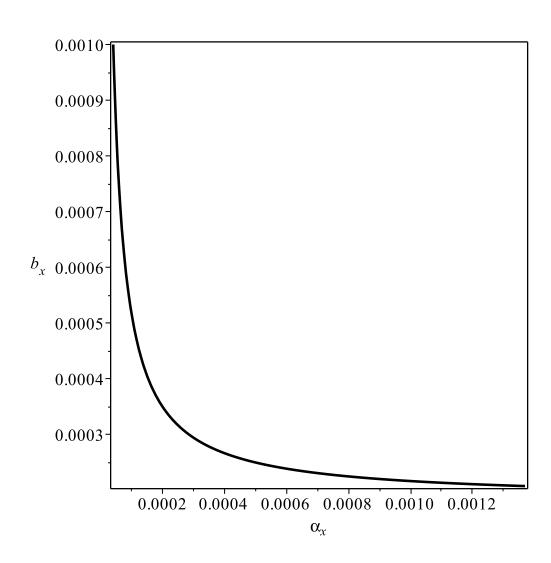
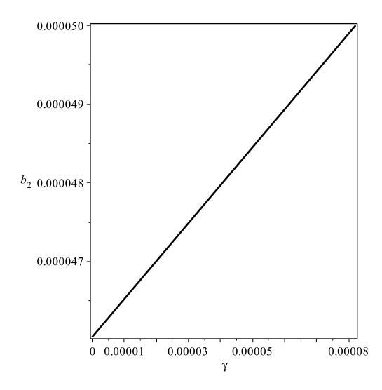
Figure 3: Sensitivity of \(\mathcal{R}_{0x}\) respect to \(\alpha_x\) and \(b_x\). The black curve is when \(\mathcal{R}_{0x} = 1\). Above black curve is when \(\mathcal{R}_{0x} > 1\), and \(\mathcal{R}_{0x} < 1\) below black curve.
Figure 4: Sensitivity of \(\mathcal{R}_{0y}\) respect to \(\gamma\) and \(b_2\). The black curve is when \(\mathcal{R}_{0y} = 1\). The left hand side area of the black curve is when \(\mathcal{R}_{0x} > 1\), and \(\mathcal{R}_{0x} < 1\) in the right hand side.
We examine the effect of some parameters which still possible to varying with human intervention to the magnitude of \(\mathcal{R}_0\). The first simulation is given to see how \(\mathcal{R}_{0x}\) affected with the change of \(b_x\) and \(a_x\). Using the set of parameters mentioned before, except \(b_x\) and \(a_x\), the sensitivity of \(\mathcal{R}_{0x}\) is given in Figure 3.
Since \(\frac{\partial \mathcal{R}_{0x}}{\partial b_x} = \frac{\alpha_x}{\mu_x(\alpha_x + \mu_x)} > 0\), and \(\frac{\partial \mathcal{R}_{0x}}{\partial \alpha_x} = \frac{b_x}{(\alpha_x + \mu_x)^2} > 0\), then we can conclude that \(\mathcal{R}_{0x}\) will decrease whenever \(b_x\) and \(\alpha_x\) reduced. \(b_x\) which present the probability of success infection of BTB can be reduced using several intervention, such as with vaccination, quarantine, etc. In the other hand, reducing \(\alpha_x\) related to some intervention to prolong the incubation period of BTB, for an example with treatment intervention. The sensitivity diagram for this scenario can be seen in Figure 3.
Using these results, the autonomous simulation for system 1 using several values of \(b_x\) performed in Figure 5. It can be seen from Figure 5 that enlarging value of \(b_x\) will end up in an endemic state (red curve). In this scenario, the endemic state \(\Gamma_2\) is exist and stable, since we have that \(\mathcal{R}_{0x} < 1\) but \(\mathcal{R}_{0y} > 1\).
The next simulation is to see how \(\mathcal{R}_{0y}\) changed respect to \(\gamma\) and \(b_2\) as shown in Figure 4. Similar with previous analysis, since \(\frac{\partial \mathcal{R}_{0x}}{\partial b_2} = \frac{\alpha \left(\delta + \mu_y\right)}{\mu_y \left(\alpha + \mu_y\right) \left(\gamma + \delta + \mu_y\right)} > 0\), then increasing value of \(b_2\) will increase \(\mathcal{R}_{0y}\). In the other hand, since \(\frac{\partial \mathcal{R}_{0x}}{\partial \gamma} = -\frac{\alpha b_2 \left(\delta + \mu_y\right)}{\mu_y \left(\alpha + \mu_y\right) \left(gm + \delta + \mu_y\right)^2} < 0\), we have that increasing value of \(\gamma\) or in this case related to the recovery rate will reducing value of \(\mathcal{R}_{0y}\). Since \(b_2\) is the infection parameter that appear in human model only, reducing \(b_2\) is highly related to an intervention that related to an effort to reduce the probability of success infection, such as with reducing duration of contact between human with medical mask, quarantine to infected individual, etc. Our result also suggest that increase value of \(\gamma\) could reduce \(\mathcal{R}_{0y}\) which related to an effort to accelerate the recovering period, for an example with increasing the quality of hospital, medicine to cure infected individual, or another interventions.
The autonomous simulation for various value of \(\gamma\) that effect value of \(\mathcal{R}_{0y}\) is performed in Figure 6. It is shown that although we succeed to reduce \(\mathcal{R}_{0y}\) until less than one with proper value of \(\gamma\), the endemic equilibrium \(\Omega_3\) still exist since the value of \(\mathcal{R}_{0x}\) is still larger than one. This result confirm our analytical result in previous section that address the endemic situation of BTB could be eliminated only with partial intervention in both cattle and human populations.
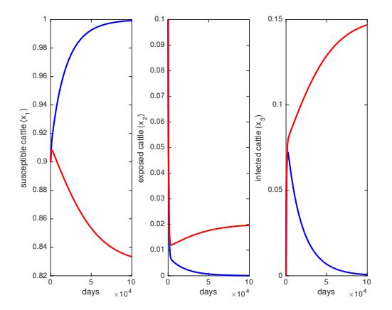
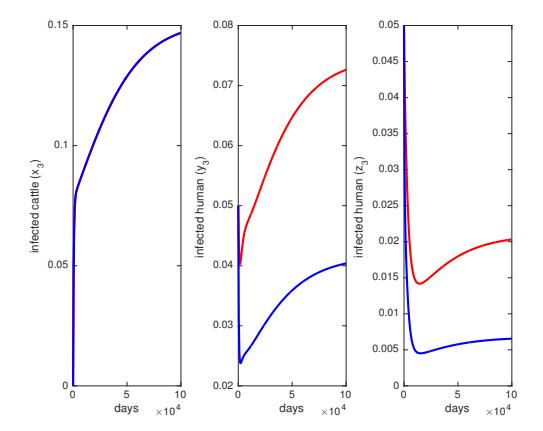
cattle (center) and infected cattle (right) with various \(b_x\). human \(y_3\) (center) and infected human \(z_3\) (right) with various The red curve is for \(\mathcal{R}_{0x}(b_x = 0.25/1000) = 1.207\), and \(\gamma\). The red curve is for \(\mathcal{R}_{0y}(\gamma = 1/(8 \times 365) = 1.598\), and \(\mathcal{R}_{0x}(b_x = 0.15/1000) = 0.725\) for the blue curve.
Figure 5: The dynamic of susceptible cattle (left), exposed Figure 6: The dynamic of infected cattle (left), infected \(\mathcal{R}_{0y}() = \gamma = 1/(2 \times 365 = 0.892 \text{ for the blue curve.}\)
5. CONCLUSIONS
A mathematical model that describes the spread of BTB among human and cattle populations has been formulated using an eleven-dimensional dynamical system. The main idea is to separate human individual in two big population based on their place for daily activity, that is in the cattle area (with possible contact with cattle) and in non-cattle area. The model developed in this article applies mostly to area that had above condition. Compared to many previous BTB models, this work contained three types of incident, that is between cattle to cattle, human to human, and cattle to human.
The basic reproduction number has been computed as the spectral radius of the next-generation matrix of related model. Sensitivity analysis has been performed and with the results showing that when the basic reproduction number on cattle is larger than one, then BTB will always exist in cattle and human population, even though the basic reproduction number in human is less than one. Also it was observed that several interventions could be consider to prevent or reduce the endemicity of BTB, such as reducing infection probability with medical mask intervention, quarantine on cattle, etc.
ACKNOWLEDGMENTS
This research is financially supported by the Indonesia Ministry of Research and Higher Education (Kemenristek DIKTI), with PUPT research grant scheme 2019 No. NKB-1595/UN2.R3.1/HKP.05.00/2019.