

1. INTRODUCTION
Aedes aegypti mosquito is the known vector of dengue disease, where the dengue disease is one of the most important arboviral disease affecting human. Dengue virus (DENV), consisting of four distinct serotypes, namely DENV-1, DENV-2, DENV-3 and DENV-4, is a member of Flaviviridae virus family [1]. Dengue is endemic in more than 128 countries and 3.97 billion people living in areas are exposed to the risk of dengue transmission [2]. It is suggested that the number of global dengue incidence is close to 400 million per year [3] and it is ranked second to Malaria amongst deadly mosquito-borne diseases [4]. During primary dengue infection, human infected by single dengue serotype will obtain life-long immunity to that serotype, but temporary partial immunity to the other three [5]. During secondary infection, the induced cross-reactive antibodies combine with the second infecting virus. Antibody-dependent enhancement (ADE) occurs and the number of infected cells increases. The ADE mechanism would result in vascular permeability and plasma leakage, leading to dengue shock and death. Hence, the ADE effect would cause human re-infected with different dengue serotype to have a higher risk of developing dengue hemorrhage fever (DHF) and dengue shock syndrome (DSS) ([6]−[8]).
The first dengue vaccine, Dengvaxia which is developed by Sanofi Pasteur, has been approved in more than 10 countries [9]. Since the licensure of Dengvaxia, there has been a raising concern about its application especially in seronegative individuals ([10]−[12]). On December 2017, the Philippines suspended schoolbased dengue vaccination programme due to the safety of Dengvaxia [13]. A supplemental statement from the World Health Organization (WHO) on 22 December 2017, verifies that there is a higher risk of severe dengue and hospitalizations among seronegative participants, regardless of age at vaccination [14]. A possible explanation is vaccination in seronegative individuals acts as a primary-like infection. The subsequent infection (first natural infection) behaves as a secondary-like infection with a higher risk of severe disease [15]−[16]. One of the challenges in administrating Dengvaxia is how to vaccinate those who will benefit from vaccination and shield those who are at risk to vaccine aquired enhanced dengue virus disease. Hence, the information on proportion of seropositive and seronegative human population to be vaccinated is vital prior to the vaccination
2 CHAI JIAN TAY
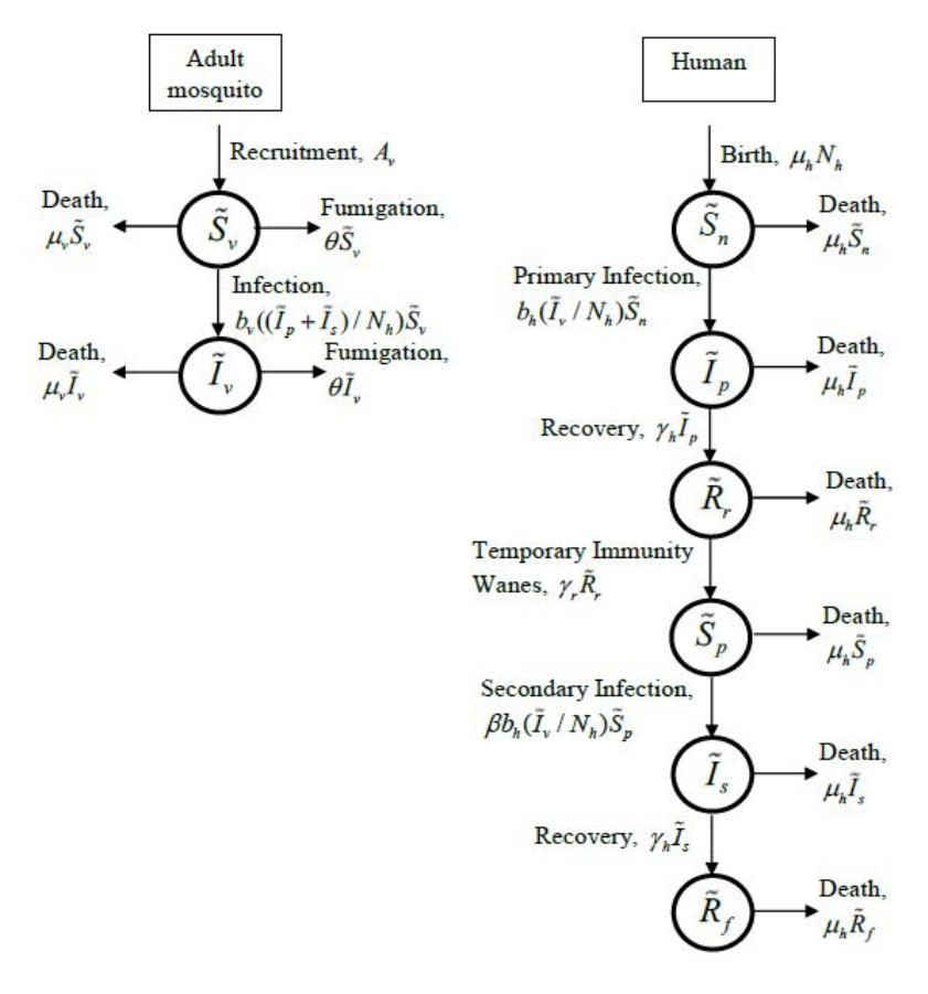
Figure 1: Compartments in the secondary dengue infection model.
program. It is also important to understand the dynamical behavior of dengue that involves both seronegative and seropositive human population. For such purpose, a secondary dengue infection model that includes both seronegative and seropositive human population is developed and investigated in this paper.
2. MATHEMATICAL MODEL
In this dengue model, both the mosquito and human populations are considered. The mosquito population is divided into susceptible, Sv, and infected, Iv, mosquitoes. The human population is classified into susceptible seronegative human, Sn, human with primary infection, Ip, temporary recovered human, Rr, susceptible seropositive human, Sp, human with secondary infection, Is and recovered human, Rf . The system of ordinary differential equations (ODEs) in (1) shows the governing equations for mosquito and human populations. In this model, only single serotype of dengue virus is considered. Human recovered from primary infection obtain temporary immunity. When the temporary immunity wanes, human become susceptible seropositive and there is a probability that the human obtain secondary infection. After recovering from the secondary infection, it is assumed that the immunity obtained is life-long. Figure 1 shows the compartments in the secondary dengue infection model while Table I shows the definition and unit of the parameters in the model.
\[\frac{d\widetilde{S}_{v}}{dt} = A_{v} - b_{v} \frac{\widetilde{I}_{p} + \widetilde{I}_{s}}{N_{h}} \widetilde{S}_{v} - \mu_{v} \widetilde{S}_{v} - \theta \widetilde{S}_{v}, \frac{d\widetilde{I}_{v}}{dt} = b_{v} \frac{\widetilde{I}_{p} + \widetilde{I}_{s}}{N_{h}} \widetilde{S}_{v} - \mu_{v} \widetilde{I}_{v} - \theta \widetilde{I}_{v}, \frac{d\widetilde{S}_{n}}{dt} = \mu_{h} N_{h} - b_{h} \frac{\widetilde{I}_{v}}{N_{h}} \widetilde{S}_{n} - \mu_{h} \widetilde{S}_{n}, \frac{d\widetilde{I}_{p}}{dt} = b_{h} \frac{\widetilde{I}_{v}}{N_{h}} \widetilde{S}_{n} - \gamma_{h} \widetilde{I}_{p} - \mu_{h} \widetilde{I}_{p}, \frac{d\widetilde{R}_{r}}{dt} = \gamma_{h} \widetilde{I}_{p} - \gamma_{r} \widetilde{R}_{r} - \mu_{h} \widetilde{R}_{r}, \frac{d\widetilde{S}_{p}}{dt} = \gamma_{r} \widetilde{R}_{r} - \beta b_{h} \frac{\widetilde{I}_{v}}{N_{h}} \widetilde{S}_{p} - \mu_{h} \widetilde{S}_{p}, \frac{d\widetilde{I}_{s}}{dt} = \beta b_{h} \frac{\widetilde{I}_{v}}{N_{h}} \widetilde{S}_{p} - \gamma_{h} \widetilde{I}_{s} - \mu_{h} \widetilde{I}_{s}, \frac{d\widetilde{R}_{f}}{dt} = \gamma_{h} \widetilde{I}_{s} - \mu_{h} \widetilde{R}_{f}.\] (1)
Table 1: Definition and unit of the parameters in secondary dengue infection model.
| Parameters | Definitions | Units | Values | References |
|---|---|---|---|---|
| \(\widetilde{S}_v\) | Susceptible adult female mosquito (wing form) | capita | - | - |
| \(\widetilde{I}_v\) | Infected adult female mosquito (wing form) | capita | - | - |
| \(\widetilde{S}_n\) | Susceptible seronegative human | capita | - | - |
| \[\begin{array}{l} \widetilde{S}_v \\ \widetilde{I}_v^{} \\ \widetilde{S}_n^{} \\ \widetilde{I}_p^{} \\ \widetilde{R}_r^{} \\ \widetilde{S}_p^{} \\ \widetilde{I}_s^{} \\ \widetilde{R}_f^{} \end{array}\] | Human with primary infection | capita | - | - |
| \(\widetilde{R}_r\) | Temporary recovered human | capita | - | - |
| \(\widetilde{S}_{p}\) | Susceptible seropositive human | capita | - | - |
| \(\widetilde{I}_s\) | Human with secondary infection | capita | - | - |
| \(\widetilde{R}_f\) | Recovered human | capita | - | - |
| t | Time | day | - | - |
| \(N_h\) | Total human population | capita | 50,000 | Assumed |
| \(A_v\) | Mosquito recruitment rate | capita \(day^{-1}\) | 5,000 | [17] |
| \(b_v\) | Dengue transmission from human to mosquito | \(day^{-1}\) | 0.33*0.75 | [17], [18] |
| \(b_h\) | Dengue transmission from mosquito to human | \(day^{-1}\) | 0.33*0.75 | [17], [18] |
| \(\mu_v\) | Natural mortality of mosquito | \(day^{-1}\) | 0.1 | [19] |
| \(\theta\) | Reduction rate of mosquito due to fumigation | \(day^{-1}\) | 0 | Assumed |
| \(\mu_h\) | Natural birth/mortality of human | \(day^{-1}\) | 0.00004 | [20] |
| \(\gamma_h\) | Human recovery rate | \(day^{-1}\) | 0.1428 | [17] |
| \(\gamma_r\) | Temporary immunity | \(day^{-1}\) | 1/180 | Assumed |
| β | Secondary infection index | 0.5 | Assumed |
The system of ODEs in (1) is scaled with the following: \(S_v = \frac{\widetilde{S}_v}{N_v}\), \(I_v = \frac{\widetilde{I}_v}{N_v}\), \(S_n = \frac{\widetilde{S}_n}{N_h}\), \(I_p = \frac{\widetilde{I}_p}{N_h}\), \(R_r = \frac{\widetilde{R}_r}{N_h}\), \(S_p = \frac{\widetilde{S}_p}{N_h}\), \(I_s = \frac{\widetilde{I}_s}{N_h}\), \(I_s = \frac{\widetilde{R}_f}{N_h}\) and \(\rho = \frac{N_v}{N_h}\). The following reduced model is obtained:
\[\frac{dS_{v}}{dt} = \mu_{v} - b_{v}(I_{p} + I_{s})S_{v} - \mu_{v}S_{v} - \theta S_{v},\] \[\frac{dI_{v}}{dt} = b_{v}(I_{p} + I_{s})S_{v} - \mu_{v}I_{v} - \theta I_{v},\] \[\frac{dS_{n}}{dt} = \mu_{h} - b_{h}\rho I_{v}S_{n} - \mu_{h}S_{n},\] \[\frac{dI_{p}}{dt} = b_{h}\rho I_{v}S_{n} - \gamma_{h}I_{p} - \mu_{h}I_{p},\] \[\frac{dR_{r}}{dt} = \gamma_{h}I_{p} - \gamma_{r}R_{r} - \mu_{h}R_{r}\] \[\frac{dS_{p}}{dt} = \gamma_{r}R_{r} - \beta b_{h}\rho I_{v}S_{p} - \mu_{h}S_{p},\] \[\frac{dI_{s}}{dt} = \beta b_{h}\rho I_{v}S_{p} - \gamma_{h}I_{s} - \mu_{h}I_{s},\] \[\frac{dR_{f}}{dt} = \gamma_{h}I_{s} - \mu_{h}R_{f}.\] (2)
3. BASIC REPRODUCTION NUMBER
Basic reproduction number is the most crucial quantity in infectious disease epidemiology, where its value provides insight in designing control measures. Basic reproduction number is the average number of secondary cases caused by one typical infected individual in a completely susceptible population [21]. The basic reproduction number of system of ODEs (2), \(R_o\) can be obtained by using the next generation method [21]. In computing the \(R_o\), it is assumed that there is no fumigation of mosquito (\(\theta=0\)). The infected subsystem, \(x^T=(I_v,\ I_p,\ I_s)\) is considered and linearized at disease-free equilibrium to obtain a Jacobian matrix. Then, eight eigenvalues are obtained as follows: \(-\gamma_h-\mu_h\), \(-\gamma_r-\mu_h\), \(-\mu_h\), \(-\mu_h\), \(-\mu_h\), \(-\mu_v\), \(\sqrt{\frac{\rho b_h b_v}{(g m_h + \mu_h) \mu_v}}\) and \(-\sqrt{\frac{\rho b_h b_v}{(g m_h + \mu_h) \mu_v}}\). The dominant eigenvalue is the basic reproduction number, \(R_o\) which is shown in Equation (3):
\[R_o^2 = \frac{\rho b_h b_v}{(q m_h + \mu_h) \mu_v}. (3)\]
3.1. Sensitivity Analysis of Basic Reproduction Number
In order to determine the significant parameter in the model, sensitivity analysis is performed for \(R_o\). The sensitivity index of \(R_o\) that depends differentiably on a user-defined parameter p, is defined by Equation (4) [22]. The sensitivity indices show how significant each parameter is to \(R_o\). Parameter values in Table I and \(\rho = 1\) are used to perform the sensitivity analysis. Table 2 shows the sensitivity indices of \(R_o\) to the parameters \(\rho\), \(b_h\), \(b_v\), \(gm_h\), \(\mu_h\) and \(\mu_v\), while Figure 2 shows the sensitivity indices of \(R_o\) displayed in a bar chart form.
\[S_p^{R_o} = \frac{\partial R_o}{\partial p} \times \frac{p}{R_o}.\] (4)
A positive index means that an increase in the parameter value results in an increase in the \(R_o\), while a negative index means that an increase in the parameter value results in a decrease in the \(R_o\) value. From Figure 2, \(R_o\) is the most sensitive to the ratio of mosquito to human, \(\rho\), dengue transmission from human to mosquito, \(b_v\), dengue transmission from mosquito to human, \(b_h\) and natural mortality of mosquito, \(\mu_v\). This indicates that an increase (decrease) of 10% in \(\rho\), \(b_v\) or \(b_h\) will increase (decrease) \(R_o\) by 5%. For \(\mu_v\), an increase (decrease) of 10% in \(\mu_v\) would result in a decrease (increase) of 5% in \(R_o\). This implies that the mosquito population, mosquito biting rate and natural mortality of mosquito should be targeted in control strategies. These results are consistent with the results of sensitivity analysis in other studies that suggest the mosquito biting rate or/and mosquito mortality rate are major factors influencing \(R_o\) ([23] – [24]). The human recovery rate, \(\gamma_h\) also provides significant effects on \(R_o\). An increase (decrease) of 10%
| Parameters | Sensitivity Indices | ||
|---|---|---|---|
| ρ | 0.5 | ||
| \(b_v\) | 0.5 | ||
| \(b_h\) | 0.5 | ||
| \(\gamma_h\) | -0.4999 | ||
| \(\mu_v\) | -0.5 | ||
| \(\mu_h\) | -0.0001 | ||
Table 2: Sensitivity indices of \(R_{o,vac}\) to the parameters.
in \(\gamma_h\) would result in a decrease (increase) of 4.999% in \(R_o\). This indicates that human with higher recovery rate could help to reduce dengue transmission. Since the \(R_o\) is evaluated at DFE, Equation (3) is independent of secondary infection index, \(\beta\). This shows that the \(R_o\) can only be used to illustrate the transmissibility of primary dengue infection.
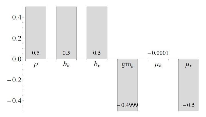
Figure 2: Sensitivity indices of \(R_o\) displayed in a bar chart form.
4. STABILITY ANALYSIS
In this section, stability analysis is performed at both disease free equilibrium (DFE), \(E_1\) and endemic equilibrium (EE), \(E_2\). First, the DFE is solved at \(\frac{dS_v}{dt} = \frac{dI_v}{dt} = \frac{dI_p}{dt} = \frac{dI_p}{dt} = \frac{dI_s}{dt} = \frac{dI_s}{dt} = \frac{dI_s}{dt} = 0\), and the following is obtained:
\[E_1 = (1, 0, 1, 0, 0, 0, 0, 0). (5)\]
The Jacobian matrix of system of ODEs (2) at DFE is obtained and Routh-Hurwitz criteria is used to prove the stability of DFE. The characteristics equation of the Jacobian matrix is:
\[\lambda^{8} + a_{0}\lambda^{7} + a_{1}\lambda^{6} + a_{2}\lambda^{5} + a_{3}\lambda^{4} + a_{4}\lambda^{3} + a_{5}\lambda^{2} + a_{6}\lambda + a_{7} = 0.\] (6)
The algebraic expressions \(a_i\) for i=0,1,2,...,7 are omitted in this paper due to space constraint. If Equation (6) has roots with negative real parts, i.e., the coefficients of \(\lambda^n\), n=0,1,2,...,8, have the same sign, then the DFE point (5) is asymptotically stable [25]. From Equation (6), the coefficient of \(\lambda^8\) is +1, which is positive, this indicates that \(a_i\), i=0,1,2,...,7 should be positive so that Equation (6) has roots with negative real parts. Since the algebraic expressions \(a_i>0, \forall i=0,1,2,...,6\) (which is omitted here due to space constraint), this implies that \(a_7>0\), as shown in expression (7):
\[\mu_h^3 \mu_v (\gamma_h + \mu_h)(\gamma_r + \mu_h)(-\rho b_h b_v + \mu_v (\gamma_h + \mu_h)) > 0.\] (7)
Since \(\mu_h\), \(\mu_v\), \((\gamma_h + \mu_h)\) and \((\gamma_r + \mu_h)\) are always greater than zero, then:
\[(-\rho b_h b_v + \mu_v (\gamma_h + \mu_h)) > 0, \tag{8}\]
\[\frac{\rho b_h b_v}{(\gamma_h + \mu_h)\mu_v} < 1. \tag{9}\]
Since \(R_o = (\rho b_h b_v)/((\gamma_h + \mu_h)\mu_v)\), thus:
\[R_o < 1. (10)\]
Hence, the DFE is locally asymptotically stable when \(R_o < 1\).
Next, the system of ODEs (2) is solved to obtain the EE as follows:
\[E_{2} = (S_{v}^{*}, I_{v}^{*}, S_{n}^{*}, I_{p}^{*}, R_{r}^{*}, S_{p}^{*}, I_{s}^{*}, R_{f}^{*}),\] \[S_{v}^{*} = \frac{\mu_{v}}{\theta + b_{v}(I_{p} + I_{s}) + \mu_{v}},\] \[I_{v}^{*} = \frac{1}{2A}(B + \sqrt{B^{2} + 4C}),\] \[S_{n}^{*} = \frac{\mu_{h}}{\rho b_{h}I_{v} + \mu_{h}},\] \[I_{p}^{*} = \frac{\rho b_{h}\mu_{h}I_{v}}{(\gamma_{h} + \mu_{h})(\rho b_{h}I_{v} + \mu_{h})},\] \[R_{r}^{*} = \frac{\gamma_{h}I_{p}}{\gamma_{r} + \mu_{h}},\] \[S_{p}^{*} = \frac{\rho b_{h}\mu_{h}\gamma_{h}\gamma_{r}I_{v}}{(\gamma_{r} + \mu_{h})(\gamma_{h} + \mu_{h})(\rho b_{h}I_{v} + \mu_{h})(\beta \rho b_{h}I_{v} + \mu_{h})} = \frac{\rho b_{h}\gamma_{h}\gamma_{r}I_{v}}{(\gamma_{r} + \mu_{h})(\gamma_{h} + \mu_{h})(\beta \rho b_{h}I_{v} + \mu_{h})} S_{n}^{*},\] \[I_{s}^{*} = \frac{\rho^{2}\beta b_{h}^{2}\mu_{h}\gamma_{h}\gamma_{r}I_{v}^{2}}{(\gamma_{r} + \mu_{h})(\gamma_{h} + \mu_{h})^{2}(\rho b_{h}I_{v} + \mu_{h})(\beta \rho b_{h}I_{v} + \mu_{h})},\] \[R_{f}^{*} = \frac{\gamma_{h}I_{s}}{\mu_{h}},\] \[(11)\] where
\[A = \beta \rho^{2} b_{h}^{2} (\theta + \mu_{v}) (b_{v} \mu_{h} \gamma_{h} \gamma_{r} + b_{v} \mu_{h} (\gamma_{r} + \mu_{h}) (\gamma_{h} + \mu_{h}) + (\gamma_{r} + \mu_{h}) (\gamma_{h} + \mu_{h})^{2} (\theta + \mu_{v})),\] \[B = \rho b_{h} \mu_{h} (\beta \rho b_{h} b_{v} (\gamma_{h} \gamma_{r} + (\gamma_{h} + \mu_{h}) (\gamma_{r} + \mu_{h})) \mu_{v} - (\gamma_{h} + \mu_{h}) (\gamma_{r} + \mu_{h}) (\theta + \mu_{v})\] \[(\gamma_{h} (1 + \beta) (\theta + \mu_{v}) + \mu_{h} (b_{v} + (1 + \beta) (\theta + \mu_{v})))),\] \[C = 4\beta \rho^{2} b_{h}^{2} \mu_{h}^{2} (\gamma_{r} + \mu_{h}) (\gamma_{h} + \mu_{h}) (\theta + \mu_{v}) (b_{v} \gamma_{h} \gamma_{r} \mu_{h} + b_{v} \mu_{h} (\gamma_{r} + \mu_{h}) (\gamma_{h} + \mu_{h})\] \[+ (\gamma_{h} + \mu_{h})^{2} (\gamma_{r} + \mu_{h}) (\theta + \mu_{v})) (\rho b_{h} b_{v} \mu_{v} - (\gamma_{h} + \mu_{h}) (\theta + \mu_{v})^{2}).\] \[(12)\]
By considering \(I_v^*\) which is a real number and always positive, we have:
\[\sqrt{B^{2} + 4C} > 0,\] \[C > 0,\] \[\rho b_{h} b_{v} \mu_{v} - (\gamma_{h} + \mu_{h})(\theta + \mu_{v})^{2} > 0,\] \[\frac{\rho b_{h} b_{v} \mu_{v}}{(\gamma_{h} + \mu_{h})(\theta + \mu_{v})^{2}} > 1.\] (13)
By letting \(\theta = 0\), we have:
\[\frac{\rho b_h b_v}{(\gamma_h + \mu_h)\mu_v} > 1,\] \[R_o^2 > 1.\] (14)
This implies that the EE is asymptotically stable when \(R_o > 1\) in the case where there is no fumigation of mosquito (\(\theta = 0\)). Next, global stability is performed at DFE by using the concept in [26]. First, the Lyapunov function is defined as:
\[V = \frac{\rho b_h}{\theta + \mu_v} I_v + I_p + I_s,\tag{15}\]
\[\frac{dV}{dt} = (-\rho b_h (1 - \beta S_p - S_n)) I_v, = ((\gamma_h + \mu_h)(R_0 - 1) - \frac{b_v b_h \rho I_v}{\mu_v + \theta}) (I_p + I_s).\] (16)
This implies that \(\frac{dV}{dt} < 0\) when \(R_0 < 1\), and consequently the DFE is globally stable.
5. NUMERICAL SIMULATIONS
In this section, numerical simulations are performed by using parameter values in Table I. Figure 3 shows the level sets of \(R_o\) in (a) \(\gamma_h\) and \(\mu_v\) planes, (b) \(b_h\) and \(\rho\) planes. From Figure 3(a), the number of dengue cases decreases when \(\mu_v\) increases. This implies that intervention such as adult mosquito insecticide can be used to reduce dengue transmission. The number of dengue cases can also be reduced when human recovery rate, \(\gamma_h\) increases. In Figure 3(b), when dengue transmission from mosquito to human, \(b_h\) increases, the dengue infection also increases. This indicates that efforts to reduce mosquito bites such as insect repellent and long-sleeved clothing could be taken to reduce dengue transmission. Figure 3(b) also shows that \(R_o\) increases when \(\rho\) increases, which implies that a higher mosquito population results in a higher dengue transmission. Intervention such as mosquito fogging could be performed to reduce the mosquito population and subsequently reduce the dengue transmission.
Besides, Figure 4 shows the level sets of (a) susceptible seronegative human, \(S_n\) and (b) susceptible seropositive human, \(S_p\) in \(\beta\) and \(\rho\) planes, respectively. An increase in the ratio of total mosquito population to total human population, \(\rho\) indicates an increase in mosquito population. When \(\rho > 1\), this implies that the total mosquito population is greater than that of human population. As a result, more human are infected by dengue and both \(S_n\) and \(S_p\) decrease. When secondary infection index, \(\beta\) increases, the risk for susceptible seropositive human to be re-infected by dengue is higher. This causes a higher transition from \(S_p\) to \(I_s\) state and the \(S_p\) population decreases.
Figure 5 displays the composition of (a) seronegative, \(S_n\) and (b) seropositive, \(S_p\) human population, respectively at dengue endemic state. The results indicate that at dengue endemic state, the composition of seronegative human population is less than 10% while the composition of seropositive human population is around 40%. By substituting parameter values in Table I, the ratio of \(\frac{S_p^*}{S_n^*}\) is 1.52, which implies that for every one seronegative individual, there exists 1.52 seropositive individual in the population. These results would provide some information on the proportion of seronegative and/or seropositive human to be vaccinated before performing the vaccination program. It should be noted that the value of 1.52 is only limited to the model and parameter values used in this paper. In an update by WHO on the use of Dengvaxia, pre-vaccination screening strategy is recommended, in which only seropositive individuals are vaccinated [27]. Further investigations are needed to identify the proportion of seronegative and/or seropositive human to be vaccinated.
Furthermore, Figure 6 shows the comparison of numerical simulations for human with (a) primary infection, \(I_p\) and (b) secondary infection, \(I_s\), respectively. It is shown that when \(I_p\) approaches zero after t=200 (Figure 6(a)), secondary dengue infection can still occur after t=200 (Figure 6(b)). This implies that a decline in primary dengue infection is not associated with decrease in secondary dengue infection. Based on epidemiological data from Thailand, [28] opined that dengue hemorrhagic fever (DHF) incidence can be effectively controlled with a sufficiently large reduction in \(R_o\) but that moderate reductions may be counterproductive. Therefore, the dengue control strategies should produce high efficacy in transmissibility reduction and ultimately to reduce the DHF.
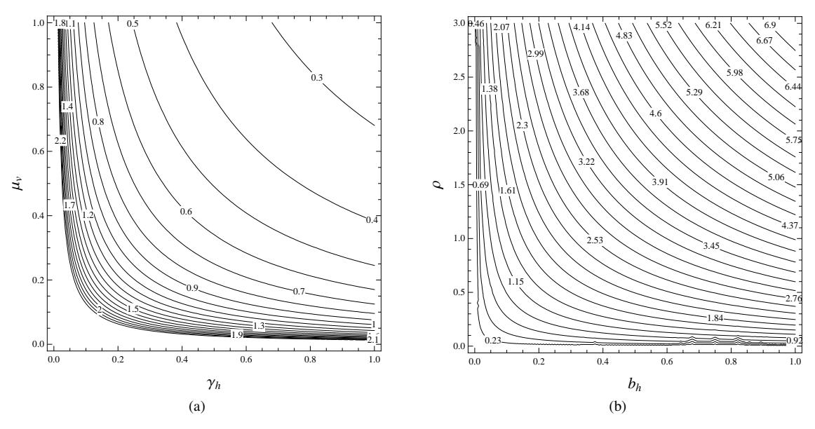
Figure 3: Level sets of Ro in (a) γh and µv planes, (b) bh and ρ planes.
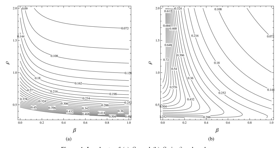
Figure 4: Level sets of (a) Sn and (b) Sp in β and ρ planes.
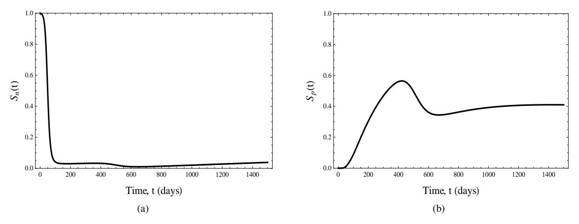
Figure 5: Comparison of composition of (a) seronegative, \(S_n\) and (b) seropositive, \(S_p\) human population, respectively at dengue endemic state.
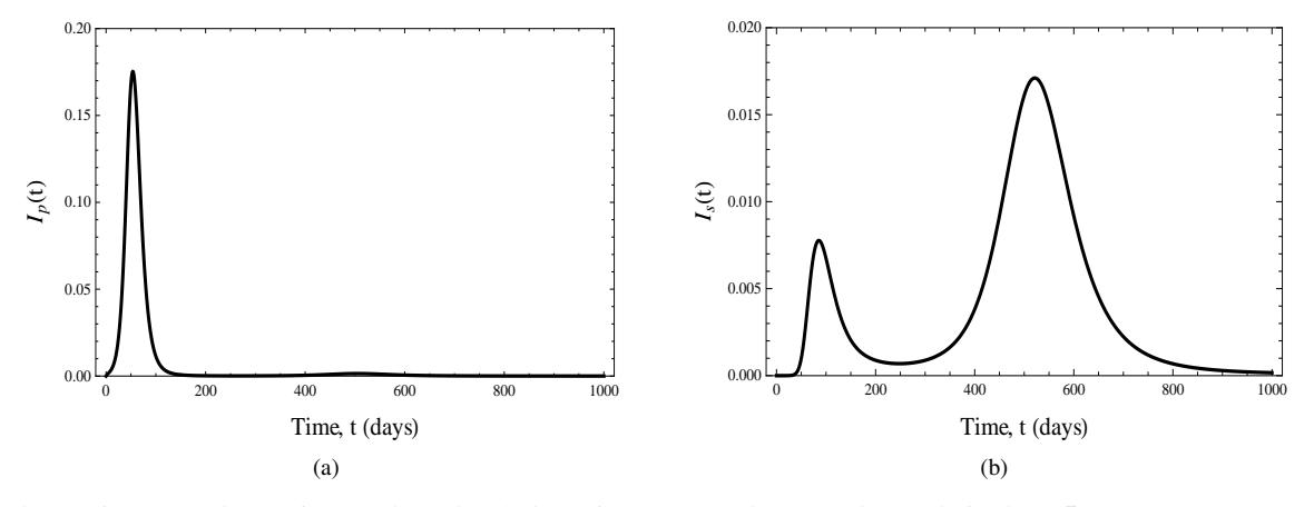
Figure 6: Comparison of numerical simulations for human with (a) primary infection, \(I_p\) and (b) secondary infection, \(I_s\), respectively.
6. CONCLUSION
In conclusion, a dengue model with secondary infection that includes both seronegative and seropositive human population is developed and investigated in this paper. The basic reproduction number, \(R_o\) is derived by using the next generation method and evaluated at DFE and EE. In stability analysis, it is shown that the DFE is asymptotically stable when \(R_o < 1\), while the EE is asymptotically stable when \(R_o > 1\) in the case where there is no fumigation of mosquito (\(\theta = 0\)). The DFE is also proved to be globally stable when \(R_o < 1\). Sensitivity analysis of \(R_o\) is performed in this paper. The results indicate that \(R_o\) is the most sensitive to the ratio of mosquito to human (\(\rho\)), dengue transmission from human to mosquito (\(b_v\)), dengue transmission from mosquito to human (\(b_h\)) and natural mortality of mosquito (\(\mu_v\)). This implies that the dengue control strategies should target on these parameters. It is indicated that the ratio of \(\frac{S_v^*}{S_v^*}\) is 1.52 at endemic state, which implies that for every one seronegative individual, there exists 1.52 seropositive individual in the population. It should be noted that the value of 1.52 is only limited to the model and parameter values used in this paper. Further investigations are needed to identify the proportion of seronegative and/or seropositive human to be vaccinated. Also, at dengue endemic state, the composition of seronegative human population is less than 10% while the composition of seropositive human population is around 40%. This would assist the decision
10 CHAI JIAN TAY
maker in deciding the proportion of seronegative and/or seropositive human to be vaccinated in vaccination program. The numerical simulations show that a decline in primary dengue infection is not associated with decrease in secondary dengue infection. Therefore, the dengue control strategies should produce high efficacy in transmissibility reduction and ultimately reduce the DHF.