

1. INTRODUCTION
Salmon is one type of fish in the family Salmonidae [1]. The other fish in the same family is Trout. Trout do not migrate, but salmon migrate. Salmon usually live in North Atlantic and Pacific Atlantic. The word "salmon" comes from the Latin "salmo" which means "to leap" [2]. They are known anadromous because their migrations have thousands of kilometers from freshwater to ocean [3]. They hatch in fresh water and then develop into smolt. After that, they go to the sea, then back to the natal stream to reproduce [4]. In the natal stream, they do spawning and after that, they die because they lost a lot of energy. This process is called semelparous. Flakes of dead salmon will be food for newly hatched alevin [5].
Not all salmon hatch and become spawning salmon because of their high mortality due to migration up to 90 percent. They have complicated immigration. Their immigration considers their behavior and physiology. They do the best communication with many inherent challenges during migration include predators, dynamic river, temperatures, and etch. Their migration is very extraordinary. They have navigation capabilities that allow them to migrate from the ocean to their original place where they were spawned. Their loyalty to returning to their spawning area is scarce between fish and other animals. They are able to adapt during immigration from salt water to fresh water. Many other fish species die when facing this challenge. But this is normal for them, although they need to overhaul the gill function and the entire osmoregulation apparatus. The other remarkable aspect is the ability not to eat during migration. They use stored energy in the form of fat. Not only it is used for immigration, but this energy is also used for the process of producing eggs or sperm. But this challenge has always been successful in dealing with Pacific salmon. Millions of Pacific salmon evidence this continuing to return to natal spawning sites along the northern edge of the Pacific. [6][7].
Predator is one of the factors in the high mortality of spawning salmon. Its element has a significant influence in determining the success of their spawning. One predator is a brown bear. Every year, they gather in large numbers along the McNeil river to prey on salmon. It is carried out when the spawning salmon return to the river [8] [9].
Because the life cycle of salmon is different from other fish, we are interested in constructing mathematical models to describe this life cycle. From this model, we can determine when we can harvest salmon as much as possible. The first chapter describes the process of the life cycle of the salmon with the predator bears. In the second chapter, the model J-A-S (Juvenile-Adult salmon-Spawning) is constructed with specific assumptions and analysis models. Lastly, by using the parameter values, sensitivity analysis and numerical simulation are shown with a variety of cases.
2. LIFE CYCLE SALMON
The life cycle of salmon begins in freshwater (especially in rivers). Here, female spawning lay 1500-7000 eggs in gravel-covered holes around Winter, and male spawning fertilizes the egg [10]. There is only 10 percent of eggs that hatch and they are called alevin [11]. The death rate after laying eggs is high because they lose energy. Alevin lives between gravel in the bottom of the river by eating plankton. In the summer, alevin comes out of the river gravel to look for food with lifetime two until three weeks. In this phase, they are called fry [12]. Fry grow and develop into juvenile in the autumn which have produced to scales and worked fins [13].
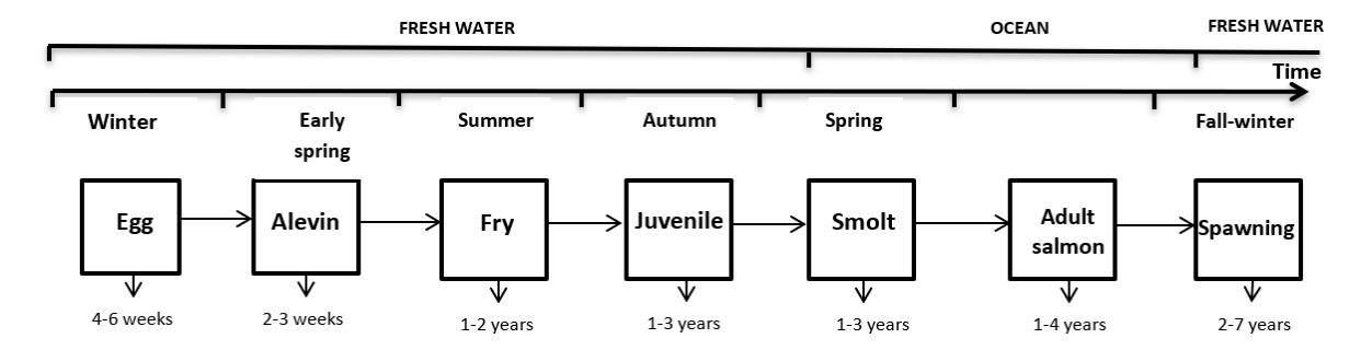
Figure 1: Generalized life cycle for pasific salmonids
The juvenile will undergo a physical change that is useful for preparing transmigration to the sea especially to survive a shift from freshwater to saltwater, and it's called smolt. Smolt will develop their body chemistry to adapt to the ocean [5]. Some types of Pacific salmon spend different time living on the river before they swim to the mouth of the river towards the ocean. Pink and Chum salmon immediately swim into the sea. Sockeye salmon spent 1-2 years, and Chinook Salmon spent five months at the river mouth. The survival of Fry depends on the high quality of habitat [5]. Smolt migrates to the mouth of the river towards the sea. Smolt grows large and turns into silver. At night to avoid predators, small salmon follow the flow of the river towards the estuary and more abundant salmon swim directly towards the sea. When at the mouth of a river, it is essential for smolt to maintain their survival and they prepare themselves to survive in the ocean. In the sea, smolt develops into adult salmon. Adult salmon are ready to lay eggs, and they colonize and return to where they came from. It's interesting that they can back to the river because they have sensors that can recognize the aroma where it originates. They are called spawning salmon. Salmon live in the sea for different times, around 4-7 years. Coho salmon are around seven years old; Pink salmon are about 18 months, Sockeye Salmon are around two years and Chinook Salmon reach around eight years before starting the journey back to the river where they lay eggs [14]. Months against the flow, over the rocks reef, jumping waterfall, and not eating during the trip because it has fat reserves in the body. This causes a physical change in the salmon, and if it does not survive it reaches the river mouth, they can die in the middle of the trip. The female parent will lay eggs, and male salmon fertilized it. Then the mothers will die slowly after laying eggs because they run out of energy [3].
3. MATHEMATICAL MODEL
Based on the lifecycle, we discuss the mathematical model of between bears and salmon with harvesting and predator factor. In this paper, the mathematical model is constructed based on the lifecycle of salmon. But not all the stages in the lifecycle of the compartment is obtained. Based on the life cycle and interaction between salmon and bears, a mathematical model is built using a differential equation system. The model includes the three compartments, i.e., Juvenile(J), Adult(A), and Spawning(S). In this model, we assume that the only spawning produce constant juvenile and we neglect the sex of all types of salmon. So, the number of J can increase because of the birth of the population S with a birth rate \(\alpha\) of spawning. Besides, only the population J compete to get foods to survive in the river and then the population J dead with the rate a. With probability \(\beta\), the population J transit from juvenile to adult salmon phase. Harvesting only occurs when salmon are in the ocean with harvesting rate h, and the population A die naturally with the rate a. After that, the bear only preys on the population spawning, so population S decrease with rate a. Based on the assumption, life cycle and interaction between three phases of salmon are shown in Figure 2.
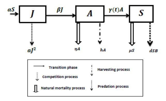
Figure 2: Flowchart of deterministic model
After reviewing the salmon life cycle along with the chronological timeline when bears meet salmon and considering the assumptions used, a logistic model is built to model the salmon population during the three phases of their life. Several factors that affect the productivity rate of salmon and these factors become parameters in the model. Hence, a normalized mathematical model is constructed in the following nonlinear differential equation system:
\[\frac{dJ}{dt} = \alpha S - aJ^2 - \beta J, \frac{dA}{dt} = \beta J - \eta A - \gamma(t)A - hA, \frac{dS}{dt} = \gamma(t)A - \mu S - dSB,\] (1)
where \(J(t)=\frac{\bar{J}(t)}{C}\), \(A(t)=\frac{\bar{A}(t)}{C}\), \(S(t)=\frac{\bar{S}(t)}{C}\), \(a=\bar{a}C\), \(d=\bar{d}C\) and \(B=\frac{\bar{B}}{C}\) with carrying capacity C and then \(0\leq\bar{J}\leq C, 0\leq\bar{A}\leq C, 0\leq\bar{S}\leq C\). We assumed that the total population of salmon are the total of juvenile, adult salmon, and spawning. Let
\[\Omega = \left\{ (J,A,S) \in \mathbb{R}^3_+ : J+A+S \leq 3 \right\}\] be any solution of system 1 with initial condition \(J(0) \ge 0\), \(A(0) \ge 0\), and \(S(0) \ge 0\). Clearly the set \(\Omega\) is positively invariant for system 1. Table 1 describes value variables and parameters that use to numerical simulation.
| Variable/ parameter | Description | Unit | Value | Source |
|---|---|---|---|---|
| \(\bar{J}(t)\) | The number of juveniles at time \(t\) | salmon | - | - |
| \(\bar{A}(t)\) | The number of adult salmons in the ocean at time \(t\) | salmon | - | - |
| \(\bar{S}(t)\) | The number of sexually mature adult salmons in freshwater at time \(t\) (Spawning) | salmon | - | - |
| \(\bar{B}\) | The number of bears at the river at time \(t\) | bear | 1500 | - |
| \(\alpha\) | Salmon birth rate | \(day^{-1}\) | [250, 800] | [10] |
| \(\bar{a}\) | Salmon death rate due to rivalry for food among the same species | \(day^{-1}\) | 0.002 | assumed |
| \(\beta\) | Transition rate from juvenile to adult phase | \(day^{-1}\) | \((\frac{1}{3*365};\frac{1}{365})\) | [5] |
| \(\gamma\) | Migration rate of adult salmon from ocean to freshwater | \(day^{-1}\) | function \(\gamma(t)\) | [5] |
| \(\eta\) | Adult salmon death rate in the ocean due to natural causes | \(day^{-1}\) | [0.005, 0.033] | [5] |
| h | Harvesting rate of adult salmons in the ocean | \(day^{-1}\) | 0.005 | [17] |
| \(\mu\) | Spawning salmon death rate in freshwater due to natural causes | day-1 | \((\frac{1}{125}; \frac{1}{66})\) | assumed |
| \(\frac{\mu}{\bar{d}}\) | Rate of bear predation on spawner salmon | day-1 | \[\left(\frac{\frac{1}{125}; \frac{1}{66}}{\frac{0.0002}{6*107}}; \frac{0.12}{6*107}\right)\] | assumed |
| C | Carrying capacity of the Juvenile salmon population | salmon | \(6*10^{7}\) | assumed |
Table 1: Description of variables and parameters
4. ANALYSIS OF EQUILIBRIUM POINT
In this section, we assume that all parameters and the proportion of bear are constant. Based on the model (1), there are two equilibria which are \(E_0 = (0,0,0)\) and \(E_1 = (J^*,A^*,S^*)\), where
\[J^* = \frac{\beta}{a}(Ro - 1),\] \[A^* = \frac{\beta^2}{a(h + \eta + \gamma)}(Ro - 1),\] \[S^* = \frac{\gamma\beta^2}{a(\mu + d\beta)(h + \eta + \gamma)}(Ro - 1),\] and
\[Ro = \frac{\alpha \gamma}{(\mu + dB)(\eta + h + \gamma)}.\]
The equilibrium \(E_0\) always exist, and it means that all three populations become extinct. On the other hand, the point \(E_1\) exists if Ro > 1. This means that the total number of juveniles produced during a salmons life and the total of adults that migrate to freshwater has to be considerably large to ensure the coexistence of \(E_1\). Next, the stability of the equilibrium points is analyzed in Theorem 4.1 and Theorem 4.2.
Theorem 4.1. The disease-free equilibrium \(E_0\) of the model (1) is locally asymptotically stable whenever Ro < 1.
Proof: Evaluate the Jacobian matrix of the system (1) at \(E_0\) as follows
\[J(E_0) = \begin{bmatrix} -\beta & 0 & \alpha \\ \beta & -\eta - \gamma - h & 0 \\ 0 & \gamma & -dB - \mu \end{bmatrix}.\]
The characteristic of the above matrix is given by
\[\lambda^3 + a_1\lambda^2 + a_2\lambda + a_3 = 0\] where
\[\begin{array}{ll} a_1 &= dB+\beta+\eta+\gamma+h+\mu, \\ a_2 &= (dB+\beta+\eta+\gamma+h+\mu)\beta+(\eta+\gamma+h)(dB+\mu), \\ a_3 &= \beta(1-Ro)(\eta+\gamma+h)(dB+\mu). \end{array}\]
If all parameter values are positive and 0 < Ro < 1, the polynomial will satisfy \(a_3 > 0\) and \(a_1a_2 - a_3 > 0\). According to Routh-Hurwitz's stability criterion, all roots of the characteristic equation are negative. Thus, the point \(E_0\) is locally asymptotically stable.
The following theorem discusses the stability of the equilibrium \(E_1\).
Theorem 4.2. If Ro > 1, the equilibrium \(E_1\) is locally asymptotically stable.
Proof: We linearize the system (1) around \(E_1\). The Jacobian matrix at \(E_1\) is given by
\[J(E_1) = \begin{bmatrix} \frac{2\beta((dB - \alpha + \mu)\gamma + (\eta + h)(dB + \mu))}{(\eta + h + \gamma)(dB + \mu)} - \beta & 0 & \alpha \\ \beta & -\eta - \gamma - h & 0 \\ 0 & \gamma & -dB - \mu \end{bmatrix}.\]
The characteristic polynomial of matrix \(J(E_1)\) is given by
\[b_1 \lambda^3 + b_2 \lambda^2 + b_3 \lambda + b_4 = 0\] where
\[\begin{array}{ll} b_1 &= (h+\eta+\gamma)(\mu+dB),\\ b_2 &= \gamma\alpha\beta+\beta b_1(Ro-1)+b_1(dB+\gamma+h+\mu+\eta),\\ b_3 &= \gamma\alpha\beta(\gamma+\eta+h+\mu)+b_1(dB+\gamma+h+\mu+\eta)(Ro-1)+b_1^2,\\ b_4 &= \beta b_1^2(Ro-1). \end{array}\]
It's clear, when Ro > 1, then coefficient \(b_1 > 0\), \(b_2 > 0\), \(b_3 > 0\), \(b_4 > 0\), and \(b_2b_3 - b_1b_4 > 0\). According to Routh-Hurwitz's stability criterion, all roots of the characteristic equation are negative. Thus the point \(E_1\) is locally asymptotically stable.
5. SENSITIVITY ANALYSIS AND NUMERICAL SIMULATION
Sensitivity analysis is essential to determine a parameter that gives a significant influence. For this sensitivity, we analyze the coexistence point, especially for adult salmon. Using parameters in table 1, except B and \(\beta\), we analyze the correlation between the portion of the bear and the transition rate from juvenile to adult salmon. Figure 3 gives information that the transition rate from juvenile to adult salmon increase and the portion of bear decay, the portion of the adult salmon increase. But if both transition rate from juvenile to adult salmon and the portion of the bear increase, they exist around \(0.6*10^{-5}\).
The numerical simulation describes behavior solution of system (1). In Figure 4, numerical solutions are shown without the rate of harvesting and with harvesting. Using parameter in Table 1, solution stable in point \(E_1\). Figure 4 explains that the portion of the juvenile is higher than the proportion of adult salmon. It is due to factors of mortality, harvesting, and transition of adult salmon to spawning. The proportion of spawning is lower than other proportion due to deaths and predators.
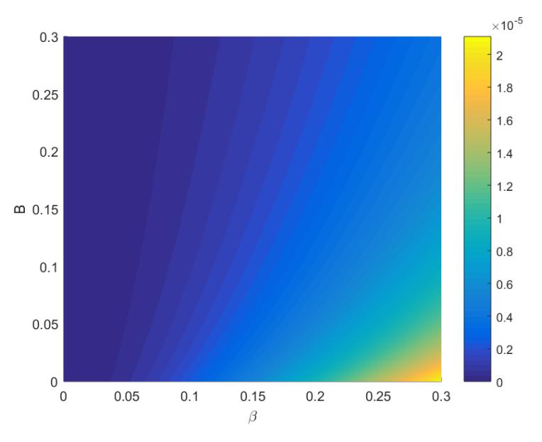
Figure 3: Sensitivity analysis: this figure shows the proportion of adult salmon for all combination parameter β and B. The color in this figure describes the proportion of adult salmon. The correlation between the A ∗ and β is quadratic but the correlation between the A ∗ and B is inverse.
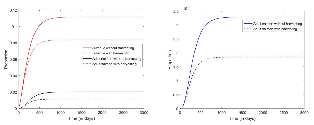
Figure 4: Behaviour solution of J(t), A(t), S(t) with constant γ(t) = 0.005
But in reality, the proportion of juvenile, adult salmon, and spawning do not always exist or constant every time. Adult salmon migrate from the ocean to the natal river around the July-September. Especially, Chinook salmon back to Columbia River dominantly in a late August [18]. Therefore, the model needs to be improved to represent the phenomenon of fact by replacing the function γ(t) as follows
\[\gamma(t) = \begin{cases} \exp(-\frac{(t-238)^2}{200}), & 202 < t \text{ mod } 365 < 365\\ 0, & otherwise. \end{cases}\]
Figure 5 shows the graph of a function γ(t) for two years. The function γ(t) explain that spawning migrates periodically once a year, especially around the July-September and peak of migrating in late August.
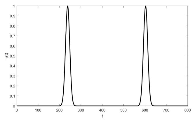
Figure 5: Function γ(t)
Numerical simulation is shown in left Figure 6 for six years. Using data on the average harvesting rate of the salmon population in the Nushagak River, Bristol Bay, i.e., h = 0.005 [17], it is clear that the proportion of juvenile, adult salmon, and spawning without harvesting are higher than the proportion of those without harvesting. The first year, we can find juvenile with an initial value of J = 0.00625 and on the first day until day 102 with the peak on the early 5 days and July. The second, third year and so on, they are found dominant around August. Then, the proportion of adult salmon is lower than the proportion of juvenile. The peak of adult salmon appear after the peak of juvenile, and it is starting from November-December of the year with a life one year. Spawning exists around August-December, and the proportion of spawning is lower than the other. The next, Figure 6 in the right describes the corresponding between juvenile, adult salmon, and spawning. If the proportion of juvenile increase, then the proportion of adult salmon and spawning increase. But, they will decrease, if the juvenile decrease. Based on the behavior of the solution, it's best to harvest adult salmon around August with not harvesting everything. Its aim is that there are still adult salmon which are prepared to become spawning so that they still lay eggs.
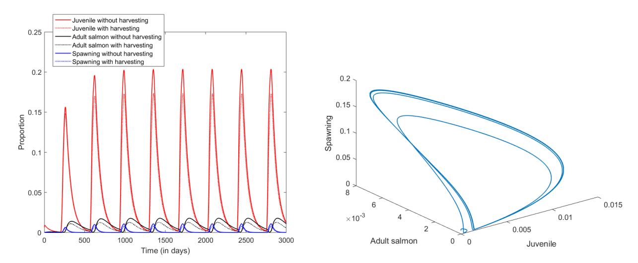
Figure 6: Behaviour solution of J(t), A(t), and S(t) with periodic function γ(t)
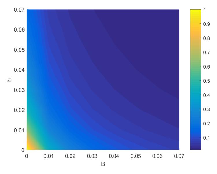
Figure 7: Sensitivity analysis: Combination parameters B and h give change ratio (R) where R is the ratio between total adult salmon during 10.9 years with h 6= 0, B 6= 0 and total of adult salmon with h = 0, B = 0.
Harvesting rate and bear increase give the ratio between total adult salmon during 10.9 years and total adult salmon without harvesting and bear close to zero. Using the average of rate harvesting in Bristol Bay, we have a ratio around 0.9, it's mean that the total population of adult salmon with h = 0.005 and B = 0.000025 is 0.9 of their total without harvesting and bear (see in Figure 7).
6. CONCLUSION
The deterministic model of the life cycle salmon has been built with a bear predator. This model consists of three compartments, namely: Juvenile, adult salmon, and spawning. Various factors that make changes in the proportion of each compartment are considered from birth, natural death, harvesting, a period of transition, and predators. Assuming all parameters is constant and the proportion of bear is constant too, we get stability conditions at the point of co-existence and not coexistence. If Ro < 1, point E0 stable and if Ro > 1 point E1 stable. Furthermore, sensitivity analysis gives information about the relationship between the portion of bears and the transition rate from juvenile to adult salmon. If the portion of bear increase and it's a transition rate increase, then the proportion of adult salmon at t → ∞ close to 0.6 ∗ 10−5 . But the proportion of adult salmon decrease and it's transition decay, they will be close to zero. Based on the stability at the point of coexistence, it is impossible that the proportion of juvenile, adult salmon, and spawning always exist or constant. So, the model is improved by replacing the migration rate with a periodic function where it's a peak around August. The numerical simulation with parameters that juvenile, adult salmon, and spawning exist predominantly only at certain times especially August. So, from this solution, we can harvest adult salmon at certain times too. The proportion of Juvenile is higher than the other and Spawning salmon is lower than the other. Using harvesting rate in Bristol Bay, the ratio between the total of adult salmon with h = 0.005, B = 0.000025 and the total without h, B close to 0.9. So, harvesting in Bristol Bay gives optimal harvesting.