

1. INTRODUCTION
Javan rhino (Rhinoceros sondaicus) is the most rare rhinoceros among the world's five rhinoceros species [9]. It has been classified as critically endangered species in the Red Data List of Threatened Species by the International Union of Conservation of Nature [6] and in Appendix I (list of the most endangered animals) of CITES (Convention on International Trade in Endangered Wild Fauna and Flora Species).
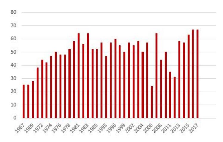
Figure 1: Population of Javan rhino between 1967-2017 from Rahmat [9] and available data at Ujung Kulon National Park.
Received November 12th, 2018, Revised November 21st, 2018 (first) and June 24th, 2019 (second), Accepted for publication July 5 th, 2019. Copyright ©2019 Published by Indonesian Biomathematical Society, e-ISSN: 2549-2896, DOI:10.5614/cbms.2019.2.1.5
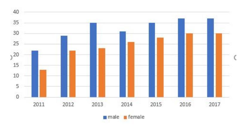
Figure 2: Population of male and female Javan rhino between 2011-2017 from available data at Ujung Kulon National Park
The number of Javan rhino's population at Ujung Kulon National Park, the only natural habitat for the Javan rhino, is shown in Figure 1 and 2. This number is far from the carrying capacity of the Ujung Kulon National Park (see [12]). Harjanto [7] tried to explain this phenomena by introducing the territorial competition that occurs between Javan rhino and Javan bull. The territorial competition is given by the nonconstant carrying capacity of Javan rhino and Javan bull that are changing with other's population's density. Unfortunately, this approach can not answer fully the phenomena. In this paper, we add the Allee effect factor in the population of Javan rhino to make a better model for the territorial competition introduced in [7].
The Allee effect, described by Warder Clyde Allee [1], is also called the negative competition effect [3]. It corresponds to the decreasing in the per-capita growth rate when the population densities is low [1]. According to Chourchamp [5], Allee effect can occur when there is genetic inbreeding which cause the loss of biodiversity, fluctuations in the sex-ratio, or the diminishing of cooperative interactions when the population is relatively low in size. Another different cause of the Allee effect according to Boukal [4] is the difficulty of finding mates when the population is relatively low.
Looking at Figure 2, it is suspected that the Allee effect occurs in the population of Javan rhino due to the difficulty of finding mates that results in inbreeding. Rahmat [9] analyzes that inbreeding in a population can cause problems in the survival of the population, such as the reduction of birth weight and fertility, that will reduce the survival of the population itself. Nowadays, there are still lots of research on the Alee effect in a predator prey type of system, see [10, 2, 11, 8]. This factor adds up an interesting dynamics to the model.
2. FORMULATION OF THE MODEL
Let R and B be the the density of Javan Rhino and Javan bull at Ujung Kulon National Park, respectively. The parameter µr and µb are the intrinsic growth rate of the Javan rhino and Javan bull, respectively. Harjanto [7] proposes the model:
\[\begin{cases} \dot{R} = \mu_r R \left( 1 - \frac{R}{C_r} \right), \\ \dot{B} = \mu_b B \left( 1 - \frac{B}{C_b} \right), \end{cases}\] (1)
with the modified carrying capacity of the Javan rhino and Javan bull:
\[C_r = \frac{C_{r0}}{1 + \epsilon B},\tag{2}\]
\[C_b = \frac{C_{b0}}{1 + \eta R},\tag{3}\]
where \(\epsilon\) and \(\eta\) is the decreasing rate of the carrying capacity of Javan rhino and Javan bull, respectively. We will add Allee effect factor to the model to make it a better approach to the phenomena observed, as follows:
\[\begin{cases} \dot{R} = \mu_r R \left(\frac{R}{K'} - 1\right) \left(1 - \frac{R}{C_r}\right), \\ \dot{B} = \mu_b B \left(1 - \frac{B}{C_b}\right), \end{cases} (4)\] with K' is Allee threshold, where \(0 < K' < C_r\).
Now, we will give interpretation of this system. Let \(C_r\) be a constant. Then
\[\text{[rumus tidak dapat ditampilkan dengan baik — lihat PDF asli]}\]
This means that if the density of Javan rhino's population is less than the Allee threshold or more than the carrying capacity of Javan Rhino, then the density of the population will decrease. On the other hand, if the density is between the Allee threshold and the carrying capacity, its density will increase. Biologically, the Allee effect will make the population extinct, when the population is low.
Normalization of The System (4)
Following the work of Harjanto [7], we normalized the Javan rhino's and Javan bull's density with respect to Javan rhino's carrying capacity, i.e. \(\bar{R} = \frac{R}{C_{r0}}\) and \(\bar{B} = \frac{B}{C_{r0}}\) and eliminating the bar we get
\[\begin{cases} \dot{R} = \mu_r R \left(\frac{R}{K} - 1\right) \left(1 - R(1 + aB)\right), \\ \dot{B} = \mu_b B \left(1 - cB(1 + bR)\right). \end{cases}\] (5)
with \(K=\frac{K'}{C_{r0}}\), \(a=\epsilon C_{r0}\), \(b=\eta C_{r0}\), and \(c=\frac{1}{\rho}=\frac{C_{r0}}{C_{r0}}\)
Table 1: Variables, parameter description, and their dimension
| Variables and Parameters | Description | Dimension or Value |
|---|---|---|
| \(\mu_r\) | Natural Javan rhino growth rate | per time |
| \(\mu_b\) | Natural Javan bull growth rate | per time |
| \(C_{r0}\) | Javan rhino carrying capacity in the absence of Javan bulls | population |
| \(C_{b0}\) | Javan bull carrying capacity in the absence of Javan rhinos | population |
| K' | the Allee threshold | population |
| \(\epsilon\) | decreasing rate of the carrying capacity of Javan rhinos | nondimensional |
| \(\eta\) | decreasing rate of the carrying capacity of Javan bulls | nondimensional |
3. Analysis of The Model with Allee Effect
Equilibria of The System (5)
There are four trivial equilibria for the system (5), that is:
- 1) (R,B) = (0,0) which is an unstable saddle,
- 2) (R,B) = (K,0) which is purely unstable,
- 3) (R, B) = (1, 0) which is unstable saddle,
- 4) \((R, B) = (0, \frac{1}{a})\) which is stable.
The nontrivial equilibrium \((R,B) = \left(K, \frac{1}{c(1+bK)}\right)\) is an unstable saddle when:
\[K\left(a\,\frac{1}{c(1+bK)}+1\right)<1\tag{6}\] and stable when the inequality sign is reversed. The other equilibrium \((R^*, B^*)\) (if it exists) must satisfies
\[ac(B^*)^2 + (c - a + bc)B^* - 1 = 0,\] (7)
\(R^* = \frac{1}{1+aB^*}.\) (8)
\[R^* = \frac{1}{1+aB^*}. (8)\]
From equation (8), it is clear that this equilibrium has a unique characteristic, that is the Javan rhino's density is inversely proportional to the the Javan bull's density.
Boundedness of Solution
Next, it can be shown that there is a compact trapping domain, that is a compact domain where every solution will enter this domain in finite time and never leaves this domain, in the first quadrant, \(\mathcal{Q} = \{(R,B): R, B \geq 0\}\) for the system (5). Thus, it will prove the boundedness of solution for every initial condition in \(\mathcal{Q}\)
Lemma 3.1 (Trapping Domain of System (5) in Q). For all \(\mu_r, \mu_b\), \(C_{r0}\), \(C_{b0}\), \(\eta\), \(\epsilon\), \(K' < C_r\), \(p > \frac{1}{c}\), and q > 1, then the compact domain \(\mathcal{D} = \{(R, B) : 0 \le R, B \le \max\{p, q\}\}\) is invariant under the flow of the solution of system (5), that is the trapping domain of system (5) in Q
Proof: It can be shown easily that R and B axis is an invariant manifold of system (5). For every \(p > \frac{1}{c}\) and q > 1, let \(d = \max\{p, q\}\). Then we will show that the flow of solution of system (5) at R = B = d is nonpositive.
The flow with initial condition in Q at R = d is given by
\[\mu_r d\left(\frac{d}{K} - 1\right) (1 - d(1 + dB)) = \mu_r \frac{d}{K} (d - K) (1 - d - dB).\]
Thus, the flow at R=d is nonpositive, because \(d-K\geq 0\) and \(1-d\leq 0\). The flow at B=d is given by
\[\mu_b d (1 - cd(1 + bR)) = \mu_b d (1 - cd - bcdR),\] and it is nonpositive because \(1 - cd \le 0\). This means for every large p and q, the solution will enter this domain.
Analysis of Equilibrium \((R^*, B^*)\)
There are at most two equilibria that satisfy equation (7) and (8). From equation (7), it can be concluded that there is only one equilibrium that has meaning biologically (that is in Q). Thus, the last nontrivial equilibrium in Q is given by:
\[(R^*, B^*) = \left(\frac{2c}{a + c - bc + \sqrt{(a - c - bc)^2 + 4ac}}, \frac{a - c - bc + \sqrt{(a - c - bc)^2 + 4ac}}{2ac}\right). \tag{9}\]
It can be shown later that the stability of this equilibrium is changing depends on the opposite condition of equation (6).
Bifurcation Analysis
From equilibrium in (9), it can be seen that fold bifurcation exists when \((a-c-bc)^2+4ac=0\). It means fold bifurcation can only happen when a=c=0 or equivalently when \(C_{r0}=0\). But, from the normalization process, it is known that \(C_{r0}>0\). Thus, the fold bifurcation can not occur. What we see in this problem is something similar like the system
\[\dot{x} = \alpha x^2 + 1. \tag{10}\]
In this system, at \(\alpha = 0\), there is no equilibrium, while at \(\alpha < 0\), there are always two equilibria with different sign and different stability (see Figure 3).
In our system, system (5), there are always two equilibria with different sign that vanish at some value of parameters. Unlike the normal fold bifurcation, when we see a coalescence of two equilibria, here we see the two equilibria with different stability doesn't coalesce, but suddenly vanish.
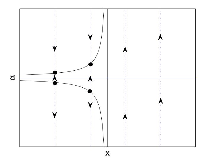
Figure 3: Bifurcation diagram of system (10). When \(\alpha \geq 0\), there is no equilibrium. While at \(\alpha < 0\), there are always two equilibria with different stability.
Another interesting bifurcation that occurs is the transcritical bifurcation. The transcritical bifurcation happen at \(\frac{1}{K}-1=a\) \(\frac{1}{c(1+bK)}\). Here, the two nontrivial equilibria are changing stability. At a certain value of parameter, there is always one that is stable, and other that is not stable (unstable saddle). The stability condition of the two equilibria can be seen at Table 2.
Table 2: The stability condition of the nontrivial equilibria
| Stability Condition | ||
|---|---|---|
| Equilibrium \((\mathbf{R}, \mathbf{B})\) | \(\mathbf{K}\left(\mathbf{a} \; \frac{1}{\mathbf{c}(1 + \mathbf{b}\mathbf{K})} + 1\right) < 1\) | \(\mathrm{K}\left(\mathrm{a}\;\frac{1}{\mathrm{c}(1+\mathrm{bK})}+1\right)>1\) |
| \((K, \frac{1}{c(1+bK)})\) | Unstable saddle | Stable |
| \((\mathbf{R}^*, \mathbf{B}^*)\) | Stable | Unstable saddle |
Thus, one will always have four trivial equilibria, and at most two nontrivial equilibria for system (5) in Q. We state the number of equilibria of the system (5) in Q by the following lemma.
Lemma 3.2 (Number of Equilibria for system (5) in Q). System (5) have at least five and at most six equilibria in Q. Four of them is the trivial equilibria with fixed stability, and the other two are nontrivial equilibria that can change stability.
4. SENSITIVITY ANALYSIS AND SIMULATION
There are three scenarios for all possible dynamics of system (5) in \(\mathcal{Q}\). The three scenarios are connected by the transcritical bifurcation with the condition (6). In all scenarios, the trivial equilibria have a fixed stability, that is unstable saddle at (0,0) and (1,0), and stable at (K,0) and \((0,\frac{1}{c})\). The nontrivial equilibria scenario undergo transcritical bifurcation.
At a certain value of parameter (without loss of generality, we choose parameter \(\epsilon\)), the equilibrium \((R^*, B^*)\) is an unstable saddle, while the other nontrivial equilibrium is stable (Figure (4) upper left). By decreasing the parameter \(\epsilon\), the two equilibria coalesce into an unstable equilibrium (Figure (4) upper right).
Later on, by decreasing the parameter more, the two nontrivial equilibrium will change their stability (Figure 4 below).
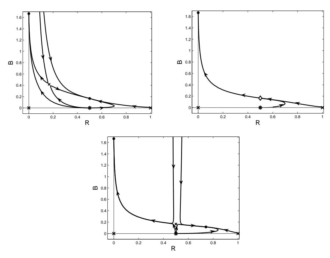
Figure 4: Phase portrait with fixed stability of nontrivial equilibria and two nontrivial equilibria. The equilibrium marked by \(\bullet\) is stable, \(\times\) is unstable saddle, * is purely unstable, and \(\diamond\) is not stable. The fixed parameters are set as follows: \(C_{r0} = 60\), \(C_{b0} = 100\), K = 30, \(\eta = 0.3\). Here, the parameter \(\epsilon\) is varied: On the upper left, the parameter \(\epsilon\) is set 0.3, while on the upper right, \(\epsilon = 0.1\). On the bottom, the parameter \(\epsilon\) is set 0.05.
Looking at the transcritical condition (6), it can be concluded that one can increase the density of Javan rhino by decreasing the Allee threshold (K'), the carrying capacity of Javan bull \((C_{b0})\), or the decreasing rate of the carrying capacity of Javan rhino \((\epsilon)\). The other ways are by increasing the carrying capacity of Javan rhino \((C_{r0})\) or the decreasing rate of Javan bull \((\eta)\).
Another interesting observation can be made by looking carefully at Figure 4 on the bottom (for instance). One can see that the domain of attraction of the stable equilibrium is formed by the stable and unstable manifold of the unstable saddle equilibrium. One can stay in this domain, if the density of the Javan rhino (R) is relatively high (in the long time, the population will stabilize to some number, see Figure 5 on the left). When the density of Javan rhino is relatively low, the Javan rhino will become extinct (stable equilibrium \(\left(0,\frac{1}{c}\right)\)) in the long time (Figure 5 on the right). This agrees with the Allee effect factor that is added to Harjanto's model [7]. In both figure, the parameter value is the same as in Figure 4 on the bottom and both have the same initial condition for Javan Bull.
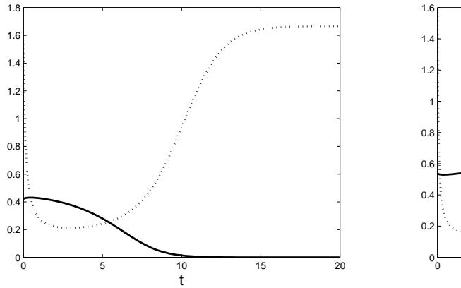
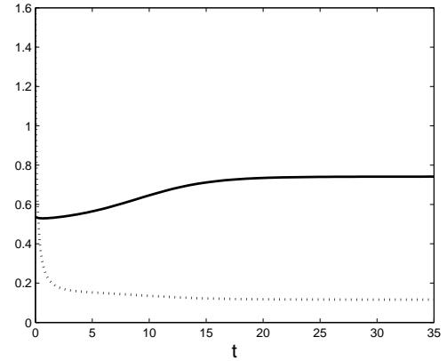
Figure 5: The graph of scaled density of Javan rhino and Bull with respect to time. The solid line is the Javan rhino's density, while the dotted line is the Javan bull's density. At relatively low density of initial condition for the Javan rhino, the population will become extinct in the long run (left). While at relatively high density of initial condition for the Javan rhino, the population will stabilize (right).
5. CONCLUSION
In this model, we give a of proof on the boundedness of the solution by using a different kind of technique than in [7]. The fold-like bifurcation that occurs in this system is discussed in great detail. It answers the question on how many equilibria can happen in the system in total. A new bifurcation, i.e. transcritical bifurcation emerges when the Allee effect factor is added. In all of the scenarios for all possible dynamics of the system, we observe that if the density of the Javan rhino's is not high enough, than in the long time, the population could become extinct.
One can increase the density of the Javan rhino by decreasing the Allee effect threshold, the carrying capacity of the Javan Bull, or the decreasing rate of the carrying capacity of Javan rhino. Other possible ways are by increasing the carrying capacity of Javan rhino or the decreasing rate of Javan bull.