

1. INTRODUCTION
In December 2019, first cases of a pneumonia of unknown cause were reported from Wuhan, China. In the meantime, these cases were identified as infections with a novel strain of coronavirus, called SARS–CoV–2, and the disease it causes was called Coronavirus Disease 2019 (COVID–19). At the beginning of January 2020, the virus spread over mainland China and reached other provinces. From 21 January onwards, WHO's daily situation reports [1] or Johns Hopkins University [2] (JHU) contain the latest figures on confirmed cases and deaths for almost all countries. In this work we rely on the data published by the JHU due to their rapid updates and easy accessibility.
The first COVID–19 case in Germany was reported on 27 January 2020 in Bavaria. Later cases were imported by travelers from China, Iran or Italy as well as tourists returning from ski holidays in Austria and Italy. By 1 March 2020, more than 100 cases were reported in Germany; since then, the number of cases began to rise exponentially. The first deaths were reported on 9 March [3]. By 16 March, the federal government introduced first measures to reduce the spread of the disease: schools, kindergartens and universities were closed. On 22 March, these measures were tightened by implementing a national curfew and contact ban. People are advised to stay at home, leaving only for work related activities, necessary shopping, medical treatment or sports [4]. By mid of April, these mitigation measures showed some success with the number of new infections declining from its peak of 6,294 on 28 March to less than 1,000 from 2 May onwards. On 6 May, a relaxation of the imposed restrictions to social and economic life was announced. Since then, the federal states are progressing at an individual pace to "normality".
Asking the population to remain cautious and not to cause a second wave, local governments of cities or districts are in charge to reinforce restrictions in case the number of new infections surpasses the limit of 50 per 100,000 inhabitants within 7 days as of 6 May [5], [6]. Already four days later five districts exceeded this limit; with no measures reported to alleviate it.
*Corresponding author
Received June 26th, 2020, Revised June 28th, 2020, Accepted for publication June 30th, 2020. Copyright ©2020 Published by Indonesian Biomathematical Society, e-ISSN: 2549-2896, DOI:10.5614/cbms.2020.3.1.5
The pandemic continues to spread worldwide (as of June 2020) and the actual possibility of a second wave demands for models to predict epidemic scenarios for the near and mid future. The quality of those models heavily relies on the parameters used. In this study we present SEIRD–models which are some sort of quasi standard in epidemiological simulations and estimate their parameters by using the available data from the JHU. The estimation itself is based on a least–squares fit between the model output and the reported data. Here, both the reported infections and the reported fatalities are taken into account.
2. Model
Following the classical SIR-models introduced by McKendrick [7] and its every-growing number of variants (cf. [8] for an overview), we chose an SEIRD-model to describe the COVID-19 outbreak in Germany. The entire population N is subdivided into five compartments: susceptibles S, exposed E, infected I, recovered R, and deceased D. The virus is transmitted from infected persons to susceptible persons at a time-dependent rate \(\beta(t)\) and after an incubation phase of duration \(\kappa^{-1}\) exposed individuals get infectious. Loss of infectivity is gained after \(\gamma^{-1}\) days and with a probability \(\mu\), a patient dies from the disease. This leads us to the following five-dimensional ODE system:
\[S' = -\frac{\beta(t)}{N}SI \qquad S(t_0) = S_0 = N - E_0 - I_0 - R_0 - D_0 > 0,\] (1a)
\[E' = \frac{\beta(t)}{N}SI - \kappa E \qquad \qquad E(t_0) = E_0 \ge 0, \tag{1b}\]
\[I' = \kappa E - \gamma I \qquad I(t_0) = I_0 > 0, \tag{1c}\]
\[R' = (1 - \mu)\gamma I R(t_0) = R_0 \ge 0, (1d)\]
\[D' = \mu \gamma I \qquad \qquad D(t_0) = D_0 \ge 0. \tag{1e}\]
The starting point \(t_0\) is chosen as 1 March as on that date number of reported cases exceeded 100 cases for the first time, see Figure 1.
It is immediate to see that the model (1) has non-negative solutions, provided the initial values are all non-negative. Due to the absence of demographic terms, there is just the trivial disease-free equilibrium S=N and E=I=R=D=0. Since the intention of our model is to provide short- and mid-term simulations, we are not interested in its long-term behavior and hence possible endemic equilibria are of no concern.
As a variant of the above basic model, we also consider a delayed differential equation (DDE) version where we introduce a time lag \(\tau\) between the infected and the deceased state so that the fraction of people who recover or die from the disease is not attained from the amount of infectives on the same day, but from the infectives data \(\tau\) days earlier. The previous ODE model can thus be seen as a special case of the DDE model with \(\tau=0\).
\[S' = -\frac{\beta(t)}{N}SI\] \(S(t_0) = S_0 > 0,\) (2a)
\[E' = \frac{\beta(t)}{N}SI - \kappa E \qquad \qquad E(t_0) = E_0 \ge 0, \tag{2b}\]
\[I' = \kappa E - \gamma \left( (1 - \mu)I + \mu I(t - \tau) \right) \qquad I(t) = \varphi(t) > 0, \tag{2c}\]
\[R' = (1 - \mu) \gamma I\] \(R(t_0) = R_0 \ge 0,\) (2d)
\[D' = \mu \gamma I(t - \tau)\] \(D(t_0) = D_0 \ge 0.\) (2e)
Here, \(\varphi:[t_0-\tau,t_0]\to\mathbb{R}_+\) denotes the initial history of the infected required for the well–posedness of the above delay differential equation. Since the initial value \(I_0\) of the infected at the starting date 1 March is later on subject of the estimation procedure, we assume the initial history to show some exponential behavior
\[\varphi(t) := I_0 \exp\left(-\frac{\ln(0.1)}{\tau} \left(t - t_0\right)\right)\] for \(t_0 - \tau \le t \le t_0\).
The transmission rate \(\beta(t)\) can be related to the Basic Reproduction Number \(\mathcal{R}_0\) via
\[\mathcal{R}_0(t) = \frac{\beta(t)}{\gamma}.\]
At the onset of the epidemic, the Basic Reproduction Number \(\mathcal{R}_0\) in Germany was estimated to be \(\mathcal{R}_0 \simeq 2.4\)—4.1, see [9]. To take the different levels of restriction imposed on the social and economic life, we assume \(\beta(t)\) as a step function in time:
\[\beta(t) := \begin{cases} \beta_0, & t < 16 \text{ March} \\ \beta_1, & 16 \text{ March} \le t < 22 \text{ March} \\ \beta_2, & 22 \text{ March} \le t < 20 \text{ April} \\ \beta_3, & 20 \text{ April} \le t \end{cases}\] \[(3)\]
Before the first restrictions were imposed on 16 March, the disease was allowed to spread almost uncontrolled. After kindergarden, school and university closings on 16 March, the measures were tightened on 22 March by introducing a contact ban and closing of a large number of shops and businesses. On 20 April, first relaxations were announced and public life began to re–increase, but along with compulsory wearing of masks which has been introduced in late April. For each of these stages we assume an specific contact rate between individuals and hence different transmission rates \(\beta_i\). The values for the fixed model parameters are given in Table 1.
Table 1: Used parameter values.
| Parameter | Value | Unit | Reference |
|---|---|---|---|
| N | 83,019,213 | - | [10] |
| \(\kappa\) | 1/3 | \(d^{-1}\) | [11] |
| \(\gamma\) | 1/10 | \(d^{-1}\) | [11] |
| \(\tau\) | > 7 | d | [11] |
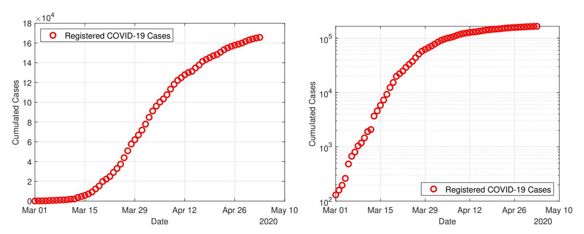
Figure 1: Graphs of cumulative infections in Germany according to Johns Hopkins University from 1 March to 3 May; on the left side with normal scaling and on the right side using semi-logarithmic scaling.
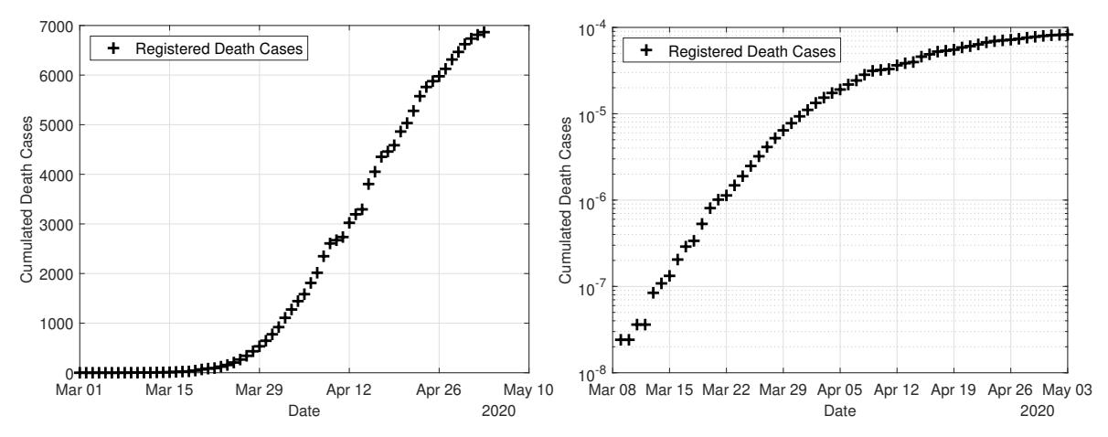
Figure 2: Graphs of cumulative death cases in Germany according to Johns Hopkins University from 1 March to 3 May. The scaling is chosen as in Figure 1.
3. PARAMETER ESTIMATION
The unknown model parameter set u is estimated from a least squares fit of the model output to the given data. Let Y and Z denote the accumulated registered COVID-19 cases or the accumulated COVID-19 deaths in Germany as reported by Johns Hopkins University, see [2]. The reported cases Y consist of the currently infected cases, the recovered and the deceased cases. Since by the very nature of the matter, not all infections are detected, we introduce a detection rate \(\delta\). For the currently infected and the recovered ones, we assume that only this proportion \(\delta\) is tested and detected and hence appears in the statistics; however, we assume no undetected deceased cases. Hence we compare the data Y to \(\delta \cdot (I+R) + D\) from the model output. To put special emphasis on the fatalities, we add a term which just compared the reported and the simulated deaths to the cost functional. As a third contribution we add a regularization term proportional to the norm of the estimated parameters to attain a convex function and prevent unrealistic outliers. With this in mind we arrive at the following cost functional:
\[J(u) := \frac{\|\delta(I+R) + D - Y\|_{L^{2}}^{2}}{\|Y\|_{L^{2}}^{2}} + \frac{\|D - Z\|_{L^{2}}^{2}}{\|Z\|_{L^{2}}^{2}} + \omega \|u\|_{2}^{2}\] \[(4)\] where \(\omega > 0\) denotes some small weight allowing us to adjust the contribution between the normalized least squares terms and the regularization term and \(\|f(t)\|_{L^2}^2 = \int_{t_0}^T f(t)^2 dt\) denotes the square of the \(L^2\)-norm of a function f resp. \(||u||_2^2 = \sum_i u_i^2\) for the square of the Euclidean norm of a vector u.
The parameters to be estimated in model (1) are the transmission rate, the detection rate, lethality and the numbers of exposed on 1 March 2020, i.e.
\[u = (\beta_0, \beta_1, \beta_2, \beta_3, \delta, \mu, E_0) \in \mathbb{R}^7\] which is the same parameter set as in model (2) with added but fixed time lag \(\tau\). For the model with free and to-be-optimized time lag \(\tau\), we have the parameter set
\[u = (\beta_0, \beta_1, \beta_2, \beta_3, \delta, \mu, \tau, E_0, I_0) \in \mathbb{R}^9.\]
Here, we also estimate the initial number of infected on 1 March to allow for more flexibility of the model. The optimal parameters \(u^*\) are determined by solving the following minimization problem:
\[\min_{u} J(u) \quad \text{subject to ODE (1) resp. (2)},\] \[u^* = \operatorname{argmin}_{u} J(u).\] (5a) (5b)
\[u^* = \operatorname{argmin}_u J(u). \tag{5b}\]
Table 2 shows the planned simulations including constraints for the optimized parameters in u.
Table 2: Simulations with the respective constraints of the fitted parameters. In Simulation 1 no time lag \(\tau\) is included in the model. The starting values for \(I_0\) and \(R_0\) are only updated in the first two simulations by division with \(\delta\) in each iteration. In Simulation 2 the time lag \(\tau=11.5\) is fixed as a mean value within the assumed interval. The parameter \(\tau\) is also fitted in Simulation 3, just like \(I_0\). All other unknown parameters in this table are adjusted in each simulation.
| - | Sim. | Model | \(\beta_i\) | δ | \(\mu\) | \(\tau\) | \(E_0\) | \(I_0\) | \(R_0\) |
|---|---|---|---|---|---|---|---|---|---|
| 1 | 1 | > 0.05 | 0.05 - 0.5 | \(\leq 0.05\) | 0 | > 0 | \(114/\delta\) | \(16/\delta\) | |
| 2 | 2 | > 0.05 | 0.05 - 0.5 | \(\leq 0.05\) | 11.5 | > 0 | \(114/\delta\) | \(16/\delta\) | |
| 3 | 2 | > 0.05 | 0.05 - 0.5 | < 0.05 | >7 | > 0 | > 0 | \(16/\delta\) |
Previous investigations in [12] already give us orders of magnitude for the initial values of the optimization for \(\beta_i\) and \(\delta\). For the lethality rate \(\mu\) we assume the upper limit
\[\mu \le \frac{Z(T)}{R(T)/\delta + Z(T)}\]
whereby Z(T) denotes for the death cases and R(T) denotes the registered recovered individuals at end time T [13]. This upper limit becomes smaller the fewer COVID cases are registered, since \(\delta\) becomes smaller. For our data set we find
\[\mu \le \frac{6866}{130600 + 6866} \approx 0.05 \tag{6}\]
based on the registered cases, i.e. this upper limit would match, if \(\delta=1\). Building on the assumption that less than 50% of cases are detected, we also assume a starting value for the lethality rate that is less than half of the calculated upper limit of 5%. The order of magnitude of the time interval between the onset of infectiousness and death is derived from the investigations in [11]. From the timelines available there we derive \(\tau \in (7,17)\). In individual cases this period can be considerably longer, so that \(\tau\) only represents an average value in the model. The starting values for \(I_0\) and \(R_0\) can be taken from the statistics. Depending on the value of the detection rate, the actual number is calculated by dividing the measured values for the infected and recovered cases by \(\delta\). Regarding an estimate of the exposed individuals \(E_0\) at time \(t_0\), we use a derivation using the Basic Reproduction Number \(\mathcal{R}_0\), which indicates how many new infections an infected individual causes on average during its illness in an otherwise susceptible population. In our model, the infected persons \(I_0\) are at different time stages during their infectiousness. As a mean value we assume the middle of this time interval. Thus, up to this point in time they could infect about \(I_0\mathcal{R}_0/2\) persons on average. Depending on the assumed Basic Reproduction Number, this results in different starting values for \(E_0\). The model adaptations are carried out in the simulations with the values \(\mathcal{R}_0 \in \{3,4,5\}\) and it is checked if significant effects on the other parameters can be found. The selected start values can be seen in Table 3.
Table 3: Orders of magnitude of the initial values for adapting the model to the available data.
| param. | \(\beta_0\) | \(\beta_1\) | \(\beta_2, \beta_3\) | δ | \(\mu\) | \(\tau\) | \(E_0\) | \(I_0\) | \(R_0\) |
|---|---|---|---|---|---|---|---|---|---|
| init. val. | 0.6 | 0.4 | 0.1 | 0.25 | 0.02 | 11.5 | \(I_0\mathcal{R}_0/2\) | \(114/\delta\) | \(16/\delta\) |
3.1. Adjoint based approach
To solve the minimization problem using adjoint functions we introduce the Lagrangian function
\[\mathcal{L}(u, x, z) = J(u) + \int_{t_0}^{T} z(t) \cdot \left( g(t, x, u) - \frac{dx}{dt} \right) dt\]
whereby \(z = (z_S, z_E, z_I, z_R, z_D)\) denotes the adjoint function regarding the state variable x = (S, E, I, R, D) and g(t, x, u) denotes the right side of the ODE resp. DDE system. It should be noted that within the integral, a scalar product of vectors is calculated. A critical point \((u^*, x^*, z^*)\) needs to fulfill the necessary optimality condition
\[\nabla \mathcal{L}\left(u^*, x^*, z^*\right) = 0.\]
For precise details of the following procedure, please refer to [14]. Thus we find the gradient \(\nabla_u \mathcal{L}\) regarding the parameters in u
\[\frac{\partial \mathcal{L}}{\partial \beta_i} = 2\omega \beta_i + \frac{1}{N} \int_{t_0}^T \frac{\partial \beta(t)}{\partial \beta_i} SI(z_E - z_S) dt, \qquad i = 0, 1, 2, 3\] (7a)
\[\frac{\partial \mathcal{L}}{\partial \delta} = 2\omega \delta + 2 \int_{t_0}^{T} (I+R) \Big( \delta(I+R) + D - Y \Big) dt, \tag{7b}\]
\[\frac{\partial \mathcal{L}}{\partial \mu} = 2\omega \mu + \gamma \int_{t_0}^{T} I(z_D - z_I) dt, \tag{7c}\]
\[\frac{\partial \mathcal{L}}{\partial E_0} = 2\omega E_0 + z_E(t_0) - z_S(t_0),\tag{7d}\]
\[\frac{\partial \mathcal{L}}{\partial I_0} = 2\omega I_0 + z_I(t_0) - z_S(t_0),\tag{7e}\]
resp. in model (2) we obtain, due to the time delay \(\tau\),
\[\frac{\partial \mathcal{L}}{\partial \mu} = 2\omega \mu + \gamma \int_{t_0}^{T} I(z_I - z_R) + I(t - \tau)(z_D - z_I) dt, \tag{7f}\]
\[\frac{\partial \mathcal{L}}{\partial \tau} = 2\omega \tau + \gamma \mu \int_{t_0}^{T} (z_I - z_D) \frac{dI}{dt} \bigg|_{t=t-\tau} dt.\] (7g)
The adjoint system is given by the equations
\[\frac{dz_S}{dt} = \frac{\beta(t)}{N} I(z_S - z_E), \qquad (8a)\]
\[\frac{dz_E}{dt} = \kappa \left( z_E - z_I \right),\tag{8b}\]
\[\frac{dz_{I}}{dt} = \frac{\beta(t)}{N} S(z_{S} - z_{E}) + \gamma (z_{I} - z_{R} + \mu (z_{R} - z_{D})) - \frac{2\delta (\delta(I + R) + D - Y)}{\|Y\|_{L^{2}}^{2}},\] (8c)
\[\frac{dz_R}{dt} = -\frac{2\delta}{\|Y\|_{L^2}^2} \left(\delta(I+R) + D - Y\right),\tag{8d}\]
\[\frac{dz_D}{dt} = -\frac{2}{\|Y\|_{L^2}^2} \left( \delta(I+R) + D - Y \right) - \frac{2}{\|Z\|_{L^2}^2} (D-Z), \tag{8e}\] with the terminal condition \((z_S, z_E, z_I, z_R, z_D)(T) = 0\). By adding the time delay in model (2) we receive
\[\frac{dz_{I}}{dt} = \frac{\beta(t)}{N} S(z_{S} - z_{E}) + (1 - \mu) \gamma(z_{I} - z_{R}) - \frac{2\delta}{\|Y\|_{L^{2}}^{2}} \left(\delta(I + R) + D - Y\right) + \mu \gamma \left(z_{I}(t + \tau) - z_{D}(t + \tau)\right) \cdot \chi_{[t_{0}, T - \tau]}(t).\] (8f)
Here \(\chi\) denotes the characteristic function
\[\chi_{[t_0,T-\tau]}(t) = \begin{cases} 1, & t \in [t_0,T-\tau] \\ 0, & \text{else} \end{cases}.\]
Algorithm 1 Pseudocode for the approach including adjoint functions.
1: u, Y, Z \leftarrow load initial values for u and data

2: x, z \leftarrow solve ODE resp. DDE for state variable and adjoint function

3: J, \nabla J \leftarrow compute objective function and gradient regarding u

4: s \leftarrow compute search direction

5: repeat

6: J_{old} \leftarrow J

7: \vartheta \leftarrow \operatorname{argmin}_{\vartheta>0} \psi(\vartheta) with \psi(\vartheta) := J(u + \vartheta s)

8: u \leftarrow u + \vartheta s

9: x, z, J, \nabla J, s \leftarrow update depending on u

10: until \|J - J_{old}\|_2 < \text{TOL}

11: u^*, x^*, z^*, J^* \leftarrow u, x, z, J
Algorithm 1 represents the basic framework of the iterative optimization via adjoint functions. To find a preferably global minimum, n multivariate normally distributed start values for u can be created before step 1. These are then tested one after the other with the presented procedure and the best result is chosen. The mean values of this distribution are then the values in Table 3, and the variances can be selected according to the restrictions in Table 2. In step 2 the ODE or DDE are solved using Runge-Kutta methods. Since the state variable is solved forward and the adjoint function backward regarding the time scale due to the initial and end values, this is also called the forward-backward sweep method [14]. In MATLAB the ode45 and dde23 solvers are suitable for this purpose. The search direction s in steps 4 and 9 is selected as Quasi-Newton method (BFGS). Useful alternative search directions are (conjugated) gradient methods [15]. The line search procedure in step 7 cannot be solved analytically in our case. A common method for an appropriate step size \(\vartheta^*\) would be a backtracking procedure considering the Armijo rule [16]. In the present simulation the procedure in Algorithm 2 is applied. It is based on a Taylor series of \(\psi(\vartheta) := J\left(u + \vartheta s\right)\) developed around \(\vartheta_0\)
\[\psi(\vartheta_0 + h) = \psi(\vartheta_0) + \psi'(\vartheta_0)h + \frac{1}{2}\psi''(\vartheta_0)h^2 + \dots\] where \(\psi', \psi'', \dots\) stand for the respective derivatives of \(\psi\) regarding \(\vartheta\). Based on this, we assume that \(\psi\) for \(\vartheta_0 = 0\) and sufficiently small values for \(h = \vartheta\) can be approximated by a parabola with
\[\psi(\vartheta) \simeq a\vartheta^2 + b\vartheta + c\] \[\psi'(\vartheta) \simeq 2a\vartheta + b.\] (9)
Using the information \(\psi(0) = J(u)\) and \(\psi'(0) = \nabla J(u) \cdot s\) associated with a calculated value \(\psi(\vartheta_1) = J(u + \vartheta_1 s)\) for small and fixed \(\vartheta_1\) allows to derive the parameters
\[c = \psi(0),\]
\[b = \psi'(0),\]
\[a = (\psi(\vartheta_1) - \psi'(0)\vartheta_1 - \psi(0))/\vartheta_1^2,\] and, by using the necessary condition \(\psi'(\vartheta^*) = 0\), find the optimum of the parabola in (9)
\[\vartheta^* = -b/(2a) = -0.5\psi'(0)\vartheta_1^2/(\psi(\vartheta_1) - \psi'(0)\vartheta_1 - \psi(0)).\]
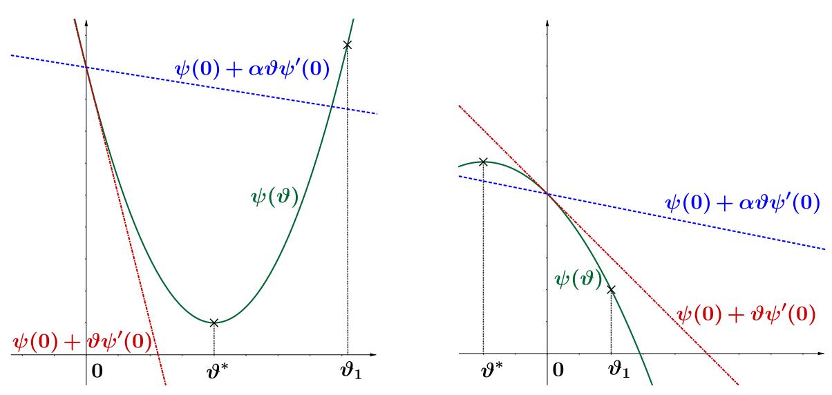
Figure 3: Graphical example to approximate the optimal value for \(\vartheta^*\) with parabola linesearch. The left figure shows that the Armijo rule \(\psi(\vartheta) \leq \psi(0) + \alpha \vartheta \psi'(0)\) is not fulfilled for \(\vartheta_1\) and the new step size is determined using the parabola minimum \(\vartheta^*\). To make sure that the possible minimum of the parabola is below that line, one chooses a small value for \(\alpha \in (0,0.5)\), e.g. \(\alpha = 1\mathrm{e}{-4}\). In the right figure the Armijo rule is already fulfilled with the fixed increment \(\vartheta_1\) which can be adopted. There can also be a parabola maximum, so that \(\vartheta^*\) takes a negative value. However, this is circumvented because in this case, there is no optimization of the step size.
Algorithm 2 Pseudocode for line search in step 7 of Algorithm 1.
1: u, J(u), \nabla J(u), s \leftarrow \text{input}
 2: \vartheta \leftarrow 1
 3: \psi(0) \leftarrow J(u)
 4: x \leftarrow compute state variable depending on u + \vartheta s
 5: \psi(\vartheta) \leftarrow J(u + \vartheta s)
 6: \psi'(0) \leftarrow \nabla J(u) \cdot s
 7: \alpha \leftarrow \text{value in } (0, 0.5)
 8: if \psi(\vartheta) > \psi(0) + \alpha \vartheta \psi'(0) then
 9:
               \vartheta \leftarrow -0.5\psi'(0)\vartheta^2/(\psi(\vartheta) - \psi'(0)\vartheta - \psi(0))
10:
               x \leftarrow \text{update depending on } u + \vartheta s
11:
               \psi(\vartheta) \leftarrow J(u + \vartheta s)
12:
           until \psi(\vartheta) \leq \psi(0) + \alpha \vartheta \psi'(0) (Armijo rule)
13:
14: end if
15: \vartheta^* = \vartheta
The effect of the weight \(\omega\) can be seen on the diagonal of the Hessian matrix in model (1)
\[\nabla_u^2 \mathcal{L} = 2 \operatorname{diag} \left( \omega, \omega, \omega, \omega, \omega + \int_{t_0}^T (I+R)^2 \, dt, \omega, \omega, \omega \right)\]
whereby all other entries in \(\nabla_u^2 \mathcal{L}\) are 0. The value of \(\omega\) directly influences the definiteness of the Hessian matrix and thus the convexity of the objective function. For this reason, different values for \(\omega\) are tested in the simulations.
3.2. Metropolis algorithm
According to the procedure described in [17], a Metropolis algorithm (cf. [18], [19], [20]) for model (2) can be set up using the initial history and initial values for the to-be-estimated parameter set \(u_0\) as of Table 3 as starting conditions, we assign random draws \(u_{new}\) from a normally distributed (and thus symmetric) proposal function q, i.e. \(u_{new} \sim q(u_{new}|u_{i-1})\), in every iteration i.
Using the previously defined J(u) as the target distribution, we calculate the approximative distribution by
\[\pi(u) = c \cdot \exp\left(-\frac{J(u)^2}{2\sigma^2}\right),\tag{10}\]
whereby c is an arbitrary value in \(\mathbb{R}\). For the acceptance probability, it follows
\[\alpha(u_{new}|u_{i-1}) = \min\left\{1, \frac{\pi(u_{new}) \cdot q(u_{i-1}|u_i)}{\pi(u_i) \cdot q(u_i|u_{i-1})}\right\} = \min\left\{1, \frac{\pi(u_{new})}{\pi(u_i)}\right\}.\](11)
In Eq.(11) we can see that the value of c is redundant as it cancels out in the division.
If the sample is accepted with the probability \(\alpha\), we set \(u_i = u_{new}\); with the probability \(1 - \alpha\), the sample is declined, meaning \(u = u_{i-1}\) [21], [17].
Algorithm 3 Pseudocode for the Metropolis algorithm.
1: u, Y, Z \leftarrow load initial values for u and data
2: x, z \leftarrow solve ODE resp. DDE for state variable
3: J \leftarrow compute objective function regarding u
4: \sigma \leftarrow standard distribution of the solution, i.e. I + R + D over time
5: s \leftarrow set step size (standard deviation) for the algorithm, e.g. s := u/100
6: repeat
7: u_{old} \leftarrow u from previous draw
8: \hat{u}_{new} \leftarrow u \sim \mathcal{N}(u_{old}, s)
9: x, z, J(\hat{u}_{new}) \leftarrow update depending on u
10: \alpha \leftarrow \min\left\{1, \exp\left(J(u_{old})^2 - J(u_{new})^2/2\sigma^2\right)\right\}
11: u_{new} \leftarrow \hat{u}_{new} with probability \alpha and u_{new} := u with probability 1 - \alpha
12: until maximum value of draws is reached
13: u^*, x^*, J^* \leftarrow means of all u, x, J
Algorithm 3 represents the basic framework of the iterative optimization via the Metropolis algorithm. In step 1, the mean values of this distribution as of Table 3 are loaded as well as the variances according to the restrictions in Table 2. In step 2 the ODE or DDE are again solved using Runge-Kutta methods via MATLAB's ode45 and dde23 solvers. The step size s in step 5 is selected as a fraction of the initial guess for the parameter set u so that the parameters are allowed move with an individual "speed" through the search space. In steps 6 to 12, the process is repeated for all draws, the number of draws in our case is set to 2e+4. Alternatively, you can think about termination conditions, but we avoided this due to the random nature of the system. Firstly, the update of the parameter set u is done by taking a random value out of the normal distribution with mean u and standard deviation s. After solving the system in step 9, the cost functional s0 s1 in step 10 and the new parameter set is accepted or rejected according to 11 in step 11. The estimation parameter set can then be computed out of the mean value of the draws in step 13. Alternatively, in case of non-convergence, you can compute the best fitting s2 of the set and use this as initial value as of step 1 again, to attain better results.
Choosing the weights \(\omega\) for the target function J(u) was done under two purposes. The first purpose was to create a convex target function so that the algorithm does not converge to local minima (see also the previous subsection for this). The Metropolis algorithm allows steps into parameter sets having a "worse" target distribution with a certain probability, but it is still possible that it runs into local but not global minima after a final amount of steps which justifies the usage of the term \(\omega ||u||^2\). The other purpose is to not have a too large \(\omega\) so that the model-related terms still have a major impact on the outcome of J(u). For these two
regards, we found that a range for \(\omega\) between \(\omega:=10^{-9}\) and \(\omega:=10^{-7}\) is decent, but we will also present the results if we neglect the term with \(\omega\), i.e. \(\omega=0\). For values \(\omega\in(0,10^{-9})\) no significant changes in the outcomes to \(\omega=0\) were detected, while for \(\omega>10^{-7}\) the model–related terms are negligible and the results are quite unrealistic.
4. NUMERICAL RESULTS AND COMPARISON OF THE ALGORITHMS
| Algorith | m Adjoint | Metropo | lis | |||
|---|---|---|---|---|---|---|
| Simulatio | n 1 | 2 | 3 | 1 | 2 | 3 |
| \(\beta_0\) | 0.60 | 0.64 | 0.62 | 0.55 | 0.70 | 0.64 |
| \(\beta_1\) | 0.50 | 0.48 | 0.51 | 0.49 | 0.40 | 0.64 |
| \(\beta_2\) | 0.101 | 0.082 | 0.092 | 0.113 | 0.085 | 0.086 |
| \(\beta_3\) | 0.099 | 0.050 | 0.058 | 0.054 | 0.055 | 0.055 |
| δ | 0.31 | 0.27 | 0.18 | 0.29 | 0.20 | 0.19 |
| \(\mu\) | 0.015 | 0.018 | 0.011 | 0.013 | 0.013 | 0.011 |
| \(\tau\) | 0 | 11.5 | 9.0 | 0 | 11.5 | 7.3 |
| \(E_0 + I_0 + R_0\) | 831 | 1,105 | 1,512 | 1,255 | 854 | 1,090 |
| \((J(u) - \omega ||u||_2^2) \cdot 10\) | \(^{3}\) 23.0 | 9.1 | 6.1 | 18.1 | 8.2 | 3.2 |
| Iterations | 23 | 22 | 31 | 20000 | 20000 | 20000 |
Table 4: Numerical Results.
Table 4 shows the respectively best numerical results of the two algorithms. The values for the transmission parameters \(\beta_i\) are of similar magnitudes in almost all simulations and algorithms. In isolated cases there are more significant deviations, such as \(\beta_1 = 0.64\) in Simulation 3 of the Metropolis approach or the value \(\beta_3 = 0.099\) in Simulation 1 of the adjoint approach. The values show that the dynamics of the model at the beginning of the measurement period with \(\beta_0 \simeq 0.6\) suggest a much higher \(\mathcal{R}_0\) than assumed. The first measures lead to a small to moderate reduction of the transmission rate to \(\beta_1 \simeq 0.5\), whereas the following lockdown causes a significant decrease of the transmission rate to \(\beta_2 \simeq 0.1\). This also fits with the estimates of the RKI that the Basic Reproduction Number is said to have dropped to a value of around \(\mathcal{R}_0 \simeq 1\) due to the extensive restrictions [3]. In the last phase of the data adaptation the transfer rate drops to \(\beta_3 \simeq 0.06\). Here, due to the loosening of the measurements, one would expect an increase of the transmission rate. However, these were introduced very slowly and under very strict hygiene measures, combined with a mask requirement in public spaces, which apparently has decreased the \(\beta\) value. Regarding the detection rate \(\delta\) we find values of around 20-30% in all cases. This means that according to the simulations, the actual number of infected people is 3-5 times higher than the official reports. The computed lethality is between 1-2% and is therefore roughly a third of 5% which was calculated in (6) regarding the registered cases at the end time point T. The average time interval \(\tau\) between the onset of infectivity and death in Simulation 3 is between 7 and 10 days. The influence of \(\tau\) is also evident with regard to the normalized least squares terms \(J(u) - \omega \|u\|_2^2\). By adding a fixed time lag in Simulation 2 and then adjusting it in the third simulation, a significant improvement is shown in all algorithms as J(u) is considerably smaller. Regarding the magnitudes of the least-squares terms, the algorithms show similar values in comparison to each other and lead to useful adjustments with minor deviations of the model from the available data sets. This is also illustrated by the graphical results which are shown in Appendices A and B. The sum of the initial values \(E_0 + I_0 + R_0\) lies within a realistic range at \(\simeq 1000\). Thus, the unknown initial value for the exposed individuals \(E_0\) is approximately in the order of magnitude of the infected \(I_0\) with an upward tendency, as expected. The variation regarding the initial value for \(E_0 = I_0 \mathcal{R}_0/2\) in the optimization does not lead to significant differences in the results when \(\mathcal{R}_0 \in \{3,4,5\}\) is changed. For this reason, the results are presented here only for initial estimations of \(\mathcal{R}_0 = 3\). In the case of the Metropolis algorithm, the number of iterations is much higher than in the adjoint approach. This is due to the fact that the Metropolis approach relies on random draws and thus a large amount of draws is needed to obtain convergence and to diminish the effect of outliers. This seemingly disadvantageous property of the Metropolis algorithm is partly counter-balanced when using n multivariate normally distributed values for u as starting guesses for the adjoint-based optimization. This also increases the iteration number by a factor n. On the other hand, this would have the consequence that the probability of reaching a global minimum for J(u) would increase significantly. This aspect is already been cared for in the Metropolis algorithm so no additional computations are required unless the chain statistics (as to be seen in the following sections). The value for J(u), especially in Simulation 3 are slightly more accurate using the Metropolis algorithm. The comparison of the runtimes in Simulation 3 on an Intel Core i5–6400 with 2.7 GHz and 16 MB–RAM also reflects this. Due to the higher number of iterations, the Metropolis algorithm also has a longer runtime, see Table 5.
Table 5: Average required runtime of the algorithms on an Intel i5–6400 with 2.7 GHz and 16 MB–RAM.
| Algorithm | Average runtime [s] |
|---|---|
| Adjoint approach | 10 |
| Metropolis | 140 |
Additionally, the influence of the weight ω on the optimization is tested. Table 6 shows the results of the least squares term J(u) − ω kuk 2 2 for Simulation 3 with the two algorithms and different weights.
Table 6: Values for the normalized least squares terms (J(u) − ω kuk 2 2 )· 103 for the optimization with different weights ω regarding the algorithms in Simulation 3.
| Algorithm | ω = 0 | ω = 10−9 | ω = 10−8 | ω = 10−7 |
|---|---|---|---|---|
| Adjoint approach | 8.9 | 8.8 | 6.1 | 12.0 |
| Metropolis | 3.8 | 3.2 | 3.4 | 4.1 |
The results show that an appropriate weight value is ω ' 10−8 resp. 10−9 , depending on the chosen algorithm. If the weight is too large, the value of the least squares term also deteriorates. This makes sense since the disturbance caused by ω kuk 2 2 on the objective function becomes too large. On the other hand, however, a sufficiently small value for ω leads to better optimization performance, since a weight of ω = 0 on the other hand gives a worse result.
4.1. Specific results for the adjoint approach
As shown in Table 4, the approach with adjoint functions leads to similar numerical results as the other tested routine. The graphical results of Simulation 3 are shown in Figure 4.
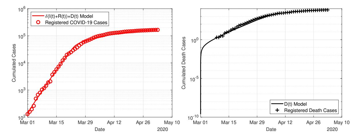
Figure 4: Plots for τ := free, E0 = free, I0 = free, R0 = 3 and ω = 10−8 .
The necessary number of iterations until the convergence of the algorithm shows that the algorithm moves quickly to the corresponding minima, see Figure 5. The process clarifies that the algorithm is very close to the optimal objective function value already after 15 iterations and needs the remaining calculation steps to reach the given tolerance limit TOL = 10−12. However, the prerequisite for rapid convergence is a good starting value for u.
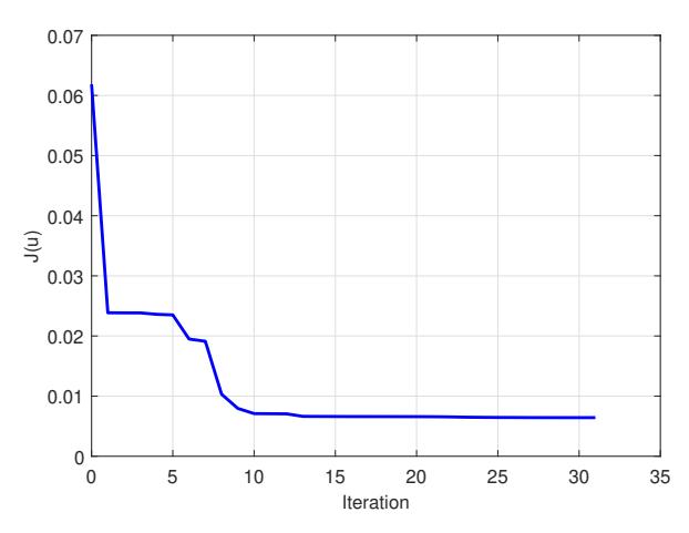
Figure 5: Development of the objective function J depending on the corresponding iteration step.
In addition to the presented simulations with restrictions, the algorithm was performed without limitations for the searched parameters, see Table 7 and Figure 6.
Table 7: Numerical results of Simulation 3 without restrictions concerning the estimated parameters.
| β0 | β1 | β2 | β3 | δ | µ | τ | E0 + I0 + R0 | 2 J(u) − kuk 2 |
|---|---|---|---|---|---|---|---|---|
| 0.77 | 0.46 | 0.27 | 0.41 | 0.002 | 0.0001 | 7 | 65046 | 7 · 10−4 |
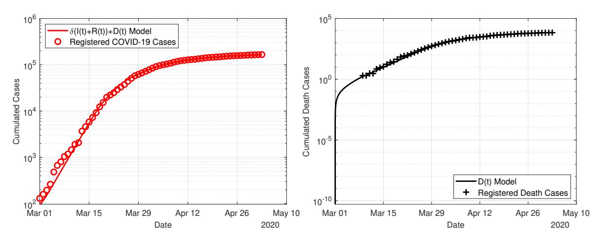
Figure 6: Graphical results of Simulation 3 without restrictions concerning the estimated parameters.
The results show that the normalized least squares term J(u)−kuk 2 2 can be reduced significantly compared to the restricted variants. It is noticeable, however, that the fitted value for the detection rate δ is very small at about 0.02%. This would mean that only every 500th infected person would be registered. This seems unrealistic, even if the dark figure is unknown. The values for transmission rate, lethality and actual number of exposed, infected and recovered at the beginning of the measurement period are changed accordingly.
Due to the very low detection rate in this simulation, the spread of the disease would have been much more intense than expected.
4.2. Specific results for the Metropolis algorithm approach
We now consider the value for
\[J(u) - \omega \|u\|_{2}^{2} = \frac{\|\delta(I+R) + D - Y\|_{L^{2}}^{2}}{\|Y\|_{L^{2}}^{2}} + \frac{\|D - Z\|_{L^{2}}^{2}}{\|Z\|_{L^{2}}^{2}},\]
i.e. the cost functional J(u) without the last term including the weight \(\omega\). This way we can compare the simulations with different weights \(\omega\) in terms of J(u) because the last term trivially raises along with \(\omega\).
Table 8: \((J(u) - \omega ||u||_2^2) \cdot 10^3\) for the different weights \(\omega\).
| Simulation | \(\omega = 0\) | \[\omega = 10^{-9}\] | \[\omega = 10^{-8}\] | \[\omega = 10^{-7}\] |
|---|---|---|---|---|
| 1 | 18.6 | 18.1 | 18.6 | 21.7 |
| 2 | 8.7 | 8.2 | 9.2 | 9.6 |
| 3 | 3.8 | 3.3 | 3.4 | 4.1 |
Table 8 shows that the weight \(\omega=10^{-9}\) always yields the best, i.e. smallest values for the given cost functional J(u). Moreover, what you can also see in Tables 10, 12 and 14 in Appendix B, the value J(u) for the weight \(\omega=10^{-9}\) is larger than the value J(u) with the weight \(\omega=0\), even when the term \(10^{-9}\cdot\|u\|_2^2\) is not subtracted, which means that interestingly, the simulation with \(\omega=10^{-9}\) provides a better result for a different cost functional.
The plots for the infected and dead cases in Simulation 3 with \(\omega = 1e-9\), thus the best simulation, are shown in Figure 7.
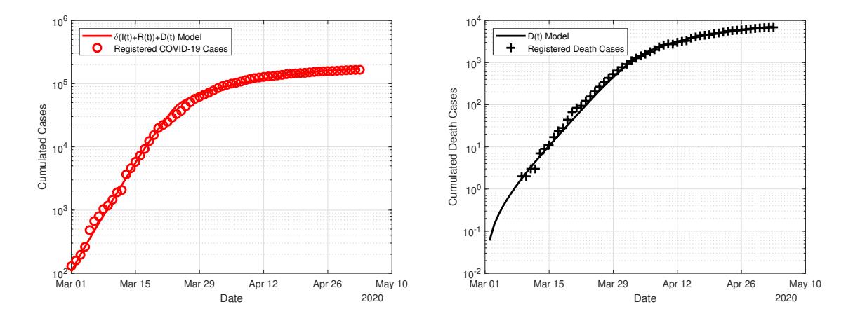
Figure 7: Plots for \(\tau =\) free, \(E_0 =\) free, \(I_0 =\) free, \(R_0 := 3\) and \(\omega = 10^{-9}\).
The chain statistics done with the optimal results in Simulation 3 for \(\omega=10^{-9}\) as of Figure 8 show that for most parameters a normal distribution is visible and thus the Metropolis algorithm appears to have converged. The parameter \(\tau\) does not appear to be normally distributed, but still remains in the range from 7–8 days. This also affects some smaller side peaks regarding the other parameters. As the infection data has the step size of 1 day, we assume that no further optimization within that range is possible, so an estimation of \(\tau\approx\) 7–8 days is decent enough.
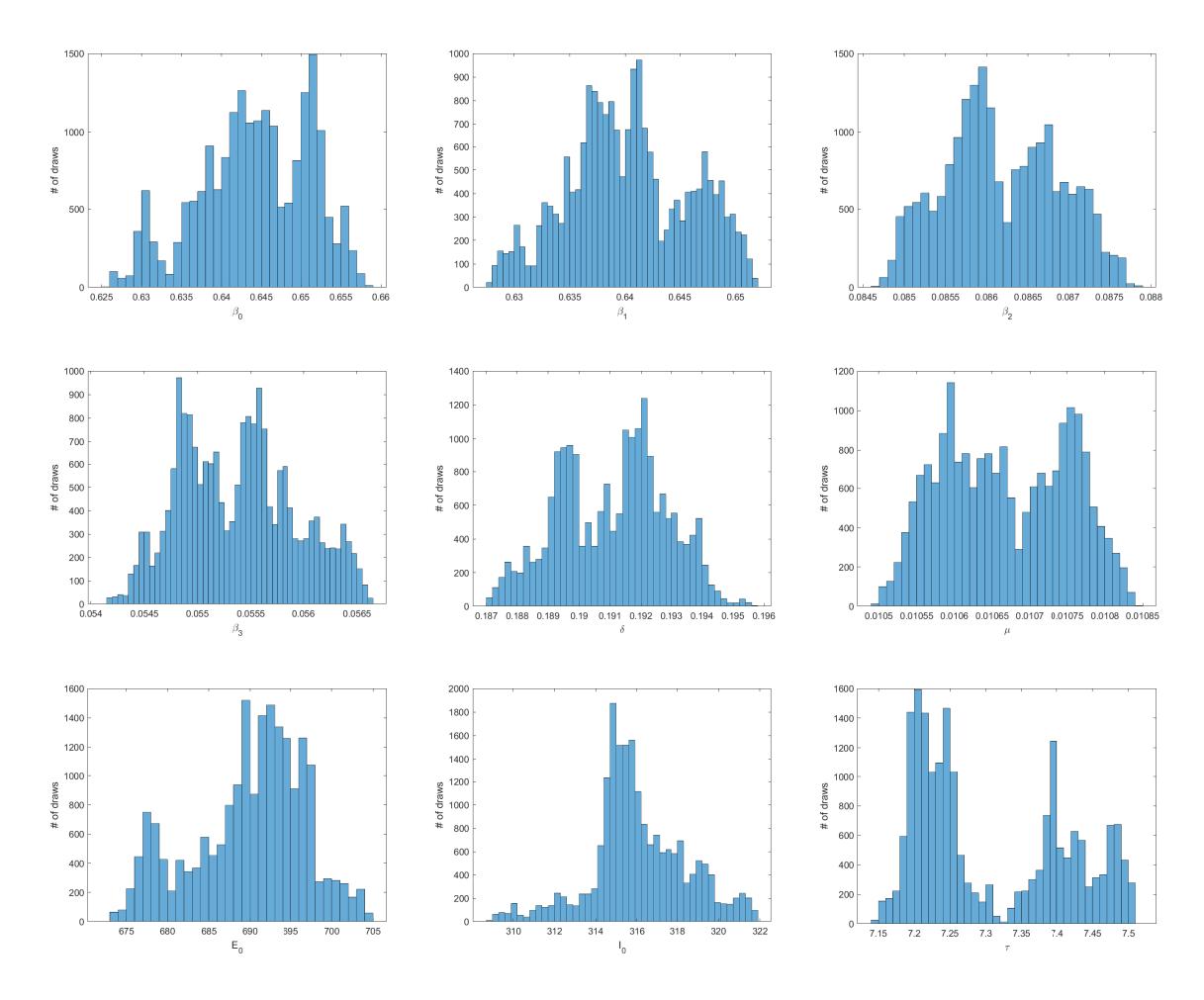
Figure 8: Parameter statistics for Simulation 2 and ω = 10−9 , using the best approximation with respect to J(u)−ω kuk 2 2 as starting value and a step size of u0/1000. Except of τ , most histograms appear roughly normally distributed around their mean values.
A detailed numerical analysis as well as figures for all relevant plots can be found in Appendix B. In the figures it is also visible that with fixed values τ = 0 or τ = 11.5 the estimated death cases run after resp. run ahead of the data.
5. CONCLUSION
In the present work, two SEIRD–models for modelling the COVID–19 outbreak in Germany were adapted to existing data from 1 March to 3 May. Two different approaches for the estimation of parameters and approximation of the infection data were used and their results and performance were compared. Regarding the graphical and numerical results, all routines have provided similar meaningful results. Each approach has advantages and disadvantages and should be selected depending on the application needs, time, possible analytical and programming effort. The Corona outbreak results show that the restrictions taken by the authorities have had a major impact on the dynamics of spread. The Basic Reproduction Number could be reduced from a presumably much higher value than the assumed R0 ' 3 to the epidemiologically important limit R0 ' 1. Adding a time lag τ between the onset of infectiousness and death significantly increases the accuracy of the tested model. This time delay is estimated by the data adjustment to an average of 8 days, although in reality there may be very different values depending on how long life-support measures are maintained in intensive care units. The adjustment regarding the detection rate and lethality showed that, according to the model, the actual number of infected people is approximately 3–5 times higher than registered and at µ ≈ 1–2%, the lethality is lower than assumed.
Conceivable extensions of the present work would be the application to other countries, the integration of travel or commuting after the relaxation of exit restrictions or the integration of control variables to mathematically derive the optimal time intervals for future lockdowns. With respect to the latter, in order to detect a new increase in infections early on – before it returns to exponential growth – a measure within the model of the possible increase in transmission rate is required.