

1. INTRODUCTION
Dengue is a vector borne disease that is transmitted to human through the bite of Aedes aegypti and Aedes albopictus mosquito [1], [2]. It is considered as one of the major public health problems in tropical and subtropical countries around the world. The first outbreak of dengue was in Philippines in 1953 and Thailand in 1955 [3]. Due to climate change and lack of public awareness the disease transmission has increased in recent years [4]. Every year 50-390 million people are infected worldwide with approximately 25,000 deaths are caused by dengue [5]. Although there is no specific medicine for dengue haemorrhagic fever (DHF), proper medical care can save life and public awareness can reduce infection [6].
Mathematical models have been widely used in several aspect to describe the transmission of dengue. A variety number of models have been developed and analyzed considering different facts of the disease. Based on the classical SIR model, the transmission has been studied in [4], [7], [8], [9], [10], [11], [12], [13], [14]. The authors in [15], [16], [17] have used the SEIR model for the study of the dynamics of dengue. In [5], [18] the authors have introduced migrated and treatment class for human population and aquatic class for vector population. In [19], the comparison of five different models of dengue fever and their best feature with performances for various scenarios have been investigated. Two host viral strains and temporary crossimmunity have been studied in [20], and a multi-strain dengue model in immunological aspects has been presented in [21].
In communicable disease modelling the incidence rate plays a vital role to describe the number of infection per unit time and by which the model gives a qualitative description of the disease dynamics. The bilinear incidence rate βSI and the standard incidence rate β(S/N)I for the classical epidemiological models [22] are
*Corresponding author
Received July 20th, 2020, Revised August 18th, 2020, Accepted for publication November 7th, 2020. Copyright ©2020 Published by Indonesian Biomathematical Society, e-ISSN: 2549-2896, DOI:10.5614/cbms.2020.3.2.2
often considered. It can be observed from the real phenomenon that the disease dynamics is not always follows these rates and many of the epidemiological mechanisms are more appropriate with nonlinear transmission rate [23]. Still now researchers have proposed several types of nonlinear incidence rate in [24], [25], [26], [27], [28], [29]. A saturated incidence rate g(I)S has been proposed by Capasso and Serio [30], after studying the spread of cholera epidemic. When a large number of infective involves in the population then exposure to the disease agent is virtually certain and the transmission rate may slow down. This happened because of the number of effective contact between the susceptible population and infected population may saturate at high infection level due to overcrowding of infective or due to protective measures by susceptible [29]. Since a large number of infective involves in vector borne disease, saturated incidence rate has been considered as more suitable for the vector borne diseases like dengue than linear incidence rates. In [5], [11], [23], [29], [31], [32] the authors have used saturated incidence rate in order to describe vector borne diseases.
Treatment is significant in every infectious disease for the infected population to become recovered. Usually, the treatment rate is considered to be proportional to the number of infective individuals. In reality, it depends on several factors such as medicines, medical resources, effectiveness of therapy, isolation process, etc. In some cases, it is observed that if the number of infectives abruptly increases then the adequate treatment becomes more challenging [33]. However, It is wise to assume a suitable treatment function for the country with a limited capacity for providing these treatment factors. In [34], Wang and Ruan introduced a constant treatment function in a SIR model. A piecewise linear treatment function has been considered by Wang in [35]. In addition, Zhou and Fan have considered the Holling type II treatment function in [24].
The recent outbreak of dengue in the year 2018 and 2019 in Bangladesh gives us a scenario of large number of infected population. As a consequence, to relate with the realistic phenomenon, we have proposed a model by considering the saturated incidence rate \(\frac{S_h I_m}{1+\alpha_1 I_m}\) and \(\frac{S_m I_h}{1+\alpha_2 I_h}\) for the transmission of human infection and mosquito infection respectively. Here \(\alpha_1\) and \(\alpha_2\) are Holling type II functional parameters. Moreover, the treatment facility becomes limited within the cities with the outgrowth of a huge number of infective. However, considering the real fact, we have considered a constant treatment function according to [34] in our model, which is defined by,
\[T(I_h) = \begin{cases} u, & \text{if } I_h > 0\\ 0, & \text{if } I_h = 0 \end{cases}\]
This simulated a limited capacity for the treatment. Here u is a positive constant represents the capacity of treatment for infective.
The formulation of the model has been described in section 2. The existence of the equilibrium points has been discussed in 3.1. The local and global stability analysis of the equilibrium have been presented in 3.2 and 3.3 respectively. Description of data for infective population and numerical simulations have been shown in section 3.4. In section 3.5 the sensitivity analysis of the parameters have been carried out. Finally, a general conclusion have been drawn in section 4.
2. MODEL FORMULATION
In order to formulate the model for dengue transmission, the interaction between two interacting populations such as human and mosquito are required. The human population have been divided into three compartments which are susceptible \((S_h)\), infected \((I_h)\) and recovered \((R_h)\). On the other hand, the mosquito population have been divided into two compartments namely susceptible \((S_m)\) and infected \((I_m)\). The total number of human population \((N_h)\) and mosquito population \((N_m)\) can be written as \(N_h(t) = S_h(t) + I_h(t) + R_h(t)\) and \(N_m(t) = S_m(t) + I_m(t)\) respectively. All new born human as well as mosquito population are considered to be infection free and susceptible. The birth rate and the death rate of human populations are considered as \(\lambda_h\) and \(\mu_h\) respectively. On the contrary, birth and death rate of mosquito populations are considered as \(\lambda_m\) and \(\mu_m\) respectively.
The dengue disease is transmitted to humans by the direct contact of infected vector and consequently, a susceptible vector becomes infected after biting an infected human. It is considered that all the susceptible and infected humans and vectors are homogeneously mixing with one another. The disease contact rate of susceptible human population due to infected mosquito population has been considered as \(\beta_m\) and the disease contact rate of susceptible mosquito population due to the infected human population has been considered as \(\beta_h\). The cases of several death are observed in different cities of Bangladesh due to dengue. Therefore, to make our model more realistic the disease-related death d has been considered. The natural recovery rate for the infected human has been considered as \(r_h\). As there is no permanent immunity from dengue and a recovered human can again be infected, so, \(\gamma_h\) has been considered as the transmission rate from recovered class to susceptible class.
Using all the assumptions, variables and parameters described above, the following system of differential equations represents our proposed model.
\[\frac{dS_h}{dt} = \lambda_h - \beta_m \frac{S_h I_m}{1 + \alpha_1 I_m} - \mu_h S_h + \gamma_h R_h\] \[\frac{dI_h}{dt} = \beta_m \frac{S_h I_m}{1 + \alpha_1 I_m} - r_h I_h - \mu_h I_h - T(I_h) - dI_h\] \[\frac{dR_h}{dt} = r_h I_h - \mu_h R_h + T(I_h) - \gamma_h R_h\] \[\frac{dS_m}{dt} = \lambda_m - \beta_h \frac{S_m I_h}{1 + \alpha_2 I_h} - \mu_m S_m\] \[\frac{dI_m}{dt} = \beta_h \frac{S_m I_h}{1 + \alpha_2 I_h} - \mu_m I_m.\] (1)
In order to make the model (1) biologically meaningful, it is necessary to prove that all the variables are non negative all of the time (t). In other words the solution of the model (1) with positive initial condition will remain positive for time \(t \ge 0\). Since the model (1) represents the interaction between the human and vector populations, it is important to state all the variables and parameters are non negative with respect to time. It is found by summing the first three equations of (1), the total human population \(N_h\) satisfies the following equation,
\[\frac{dN_h}{dt} = \lambda_h - \mu_h N_h - dI_h,\] and the total mosquito population satisfies the equation,
\[\frac{dN_m}{dt} = \lambda_m - \mu_m N_m.\]
It is easy to prove that, \(\frac{dN_h}{dt} \leq \lambda_h - \mu_h N_h\) and \(\frac{dN_m}{dt} \leq \lambda_m - \mu_m N_m\) for a special case d = 0. This follows whenever \(N_h \geq \frac{\lambda_h}{\mu_h}\) and \(N_m \geq \frac{\lambda_m}{\mu_m}\) then \(\frac{dN_h}{dt} \leq 0\) and \(\frac{dN_m}{dt} \leq 0\) respectively. On the other hand a standard comparison theorem [36] is used to show that \(0 \le (N_h, N_m) \le (N_h(0)e^{-\mu_h t} + \frac{\lambda_h}{\mu_h}(1 - e^{-\mu_h t})\)
\(N_m(0)e^{-\mu_m t}+\frac{\lambda_m}{\mu_m}(1-e^{-\mu_m t})\). Thus for \(t\to\infty,\ 0\le (N_h,N_m)\le \left(\frac{\lambda_h}{\mu_h},\frac{\lambda_m}{\mu_m}\right)\) and the region \(D=\{(S_h,I_h,R_h,S_v,I_v)\in R_+^5:N_h\le \frac{\lambda_h}{\mu_h},N_m\le \frac{\lambda_m}{\mu_m}\}\) is the positively invariant region for the model (1). Here the initial human population is considered as \(N_h^0(t)=S_h^0(t)+I_h^0(t)+R_h^0(t)=\frac{\lambda_h}{\mu_h}\) in order to get a population of a constant size [37] (that is, \(S_h(t)+I_h(t)+R_h(t)=N_h(t)=\frac{\lambda_h}{\mu_h}\)). The third equation of (1) is independent of first and second and by using \(R_h=\frac{\lambda_h}{\mu_h}-S_h-I_h\) in (1), the third equation can be eliminated. Additionally, by using the property of treatment function we found the following reduced model.
\[\frac{dS_h}{dt} = \lambda_h - \beta_m \frac{S_h I_m}{1 + \alpha_1 I_m} - \mu_h S_h + \gamma_h \left(\frac{\lambda_h}{\mu_h} - S_h - I_h\right)\] \[\frac{dI_h}{dt} = \beta_m \frac{S_h I_m}{1 + \alpha_1 I_m} - r_h I_h - \mu_h I_h - u - dI_h\] \[\frac{dS_m}{dt} = \lambda_m - \beta_h \frac{S_m I_h}{1 + \alpha_2 I_h} - \mu_m S_m\] \[\frac{dI_m}{dt} = \beta_h \frac{S_m I_h}{1 + \alpha_2 I_h} - \mu_m I_m.\] (2)
Considering \(N_{h1} = S_h + I_h\) it is found from the reduced model (2) that
\[\frac{dN_{h1}}{dt} = \lambda_h + \frac{\gamma_h \lambda_h}{\mu_h} - \mu_h N_{h1} - \gamma_h N_{h1} - (r_h + \mu_h + d)I_h - u,\] and for the mosquito population
\[\frac{dN_m}{dt} = \lambda_m - \mu_m N_m.\]
From the above equations it can be seen that in absence of disease \((I_h=0, u=0), N_{h1} \to \frac{\lambda_h}{\mu_h}\). Since the spread of the disease will reduce the population \(N_{h1}\) this follows that \(N_{h1} \in [0, \frac{\lambda_h}{\mu_h}]\). It is noted that D is the positively invariant region for the model (1) and the region
\[D_1 = \{ (S_h, I_h, S_v, I_v) \in R_+^4 : N_h \le \frac{\lambda_h}{\mu_h}, N_m \le \frac{\lambda_m}{\mu_m} \}\] is the positively invariant region for the model (2). Our goal in this paper is to analyze the global dynamics of Model (2) and investigate the transmission of dengue in Bangladesh through the model.
3. Analysis of the Model
3.1. Existence of Equilibria and Basic Reproduction Number
Disease free equilibrium (DFE) point come to light when the infections are zero and by using \(I_h = I_m = 0\)in (2), the model gives us a unique DFE which is \(E_d^0 = \left(S_h^0, I_h^0, S_m^0, I_m^0\right) = \left(\frac{\lambda_h}{\mu_h}, 0, \frac{\lambda_m}{\mu_m}, 0\right)\). To find the basic reproduction number of the model 2, the method of next generation matrix has been used and following [38], the basic reproduction number is found to be,
\[R = \sqrt{\frac{\beta_h \beta_m \lambda_h \lambda_m}{\mu_m^2 \mu_h (r_h + \mu_h + d)}}.\] (3)
Choosing, \(R_h = \frac{\beta_h \lambda_h}{\mu_h(r_h + \mu_h + d)}\) and \(R_m = \frac{\beta_m \lambda_m}{\mu_m^2}\) Equation (3) can be written as \(R = \sqrt{R_h R_m}\). Here, \(R_h\) describes the number of humans that one infectious mosquito infects over its expected infection period in a completely susceptible humans population, and \(R_m\) is the number of mosquitoes infected by one infectious human during the period of infectiousness in a completely susceptible mosquito population [31].
The endemic equilibrium points (EEP) \(E^* = (S_h^*, I_h^*, S_m^*, I_m^*)\) of the system (2) can be found by the following equations,
\[\lambda_{h} - \beta_{m} \frac{S_{h}^{*} I_{m}^{*}}{1 + \alpha_{1} I_{m}^{*}} - \mu_{h} S_{h}^{*} + \gamma_{h} \left(\frac{\lambda_{h}}{\mu_{h}} - S_{h}^{*} - I_{h}^{*}\right) = 0\] \[\beta_{m} \frac{S_{h}^{*} I_{m}^{*}}{1 + \alpha_{1} I_{m}^{*}} - r_{h} I_{h}^{*} - \mu_{h} I_{h}^{*} - u - dI_{h}^{*} = 0\] \[\lambda_{m} - \beta_{h} \frac{S_{m}^{*} I_{h}^{*}}{1 + \alpha_{2} I_{h}^{*}} - \mu_{m} S_{m}^{*} = 0\] \[\beta_{h} \frac{S_{m}^{*} I_{h}^{*}}{1 + \alpha_{2} I_{h}^{*}} - \mu_{m} I_{m}^{*} = 0.\] (4)
After calculation Equation (4) gives,
\[S_{h}^{*} = \frac{(\lambda_{h}(\mu_{h} + \gamma_{h}) - \gamma_{h}\mu_{h}I_{h}^{*}) \left(\beta_{h}(\mu_{m} + \alpha_{1}\lambda_{m})I_{h}^{*} + \mu_{m}^{2}(1 + \alpha_{2}I_{h}^{*})\right)}{\mu_{h} \left[\beta_{m}\beta_{h}\lambda_{m}I_{h}^{*} + (\mu_{h} + \gamma_{h}) \left(\beta_{h}(\mu_{m} + \alpha_{1}\lambda_{m})I_{h}^{*} + \mu_{m}^{2}(1 + \alpha_{2}I_{h}^{*})\right)\right]}\] \[S_{m}^{*} = \frac{\lambda_{m}(1 + \alpha_{2}I_{h}^{*})}{\mu_{m} + (\beta_{h} + \alpha_{2}\mu_{m})I_{h}^{*}}\] \[I_{m}^{*} = \frac{\beta_{h}\lambda_{m}I_{h}^{*}}{\mu_{m} \left(\mu_{m} + (\beta_{h} + \alpha_{2}\mu_{m})I_{h}^{*}\right)}.\]
Where \(I_h^*\) is the positive root of Equation
\[a(I_h^*)^2 + bI_h^* + c = 0, (5)\]
with
\[a = \mu_h \left[ (\beta_m \beta_h \lambda_m + (\mu_h + \gamma_h)(\mu_m \beta_h + \mu_m^2 \alpha_2 + \alpha_1 \beta_h \lambda_m)) (r_h + \mu_h + d) + \beta_m \beta_h \lambda_m \mu_h \gamma_h \right]\] \[b = \mu_h \left[ u \left( \beta_m \beta_h \lambda_m + (\mu_h + \gamma_h)(\mu_m \beta_h + \mu_m^2 \alpha_2 + \alpha_1 \beta_h \lambda_m) \right) + \mu_m^2 \mu_h (\mu_h + \gamma_h) (r_h + \mu_h + d) (1 - R^2) \right]\] \[c = u \mu_m^2 \mu_h (\mu_h + \gamma_h).\]
Here it can be seen that a>0 and c>0. By Descartes' rule of signs the only possibility for the equation (5) to have positive root if b<0. From the above equation, it is easy to find that b>0 when \(R\le 1\). Thus for \(R\le 1\) there is no positive endemic equilibrium of the model (2) and the endemic equilibrium exists for R>1. Now if R>1 i.e b<0 the number of root of Equation (5) can be determined based on the discriminant \(\Delta=b^2-4ac\). If \(\Delta>0\) then there are two positive root that means two endemic equilibrium. For \(\Delta=0\) there is one root of multiplicity 2 and for \(\Delta<0\) there is no positive root. Solving \(\Delta=b^2-4ac\) as a quadratic equation in terms of \(1-R^2\) we get \(\Delta>0\) when \(R^2>R_1^c\) or \(R^2< R_2^c\) and \(\Delta=0\) when \(R^2=R_i^c\), (i=1,2) where,
\[R_{1}^{c} = 1 - \frac{-u(\beta_{m}\beta_{h}\lambda_{m} + (\mu_{h} + \gamma_{h})(\mu_{m}\beta_{h} + \mu_{m}^{2}\alpha_{2} + \alpha_{1}\beta_{h}\lambda_{m})) + \sqrt{4ac}}{c(r_{h} + \mu_{h} + d)}\] \[R_{2}^{c} = 1 - \frac{-u(\beta_{m}\beta_{h}\lambda_{m} + (\mu_{h} + \gamma_{h})(\mu_{m}\beta_{h} + \mu_{m}^{2}\alpha_{2} + \alpha_{1}\beta_{h}\lambda_{m})) - \sqrt{4ac}}{c(r_{h} + \mu_{h} + d)}.\]
Since the case of endemic equilibrium arise for R>1, it is straightforward to write \(1 \le R_1^c < R^2 < R_2^c\). Therefore, the system (2) exhibits two endemic equilibrium if \(1 \le R_1^c < R^2 < R_2^c\) and one endemic equilibrium of multiplicity two if \(R^2=R_i^c, (i=1,2)\) and no equilibrium for other cases.
3.2. Local Stability Analysis
The local stability of the equilibrium points of the model (2) have been analyzed based on the eigenvalues of the Jacobian matrix and Routh-Hurwitz criteria. The Jacobian matrix corresponding to the system (2) around the point \(E = (S_h, I_h, S_m, I_m)\) is,
\[J(E) = \begin{pmatrix} -\frac{\beta_m I_m}{1 + \alpha_1 I_m} - \mu_h - \gamma_h & -\gamma_h & 0 & -\frac{\beta_m S_h}{(1 + \alpha_1 I_m)^2} \\ \frac{\beta_m I_m}{1 + \alpha_1 I_m} & -(r_h + \mu_h + d) & 0 & \frac{\beta_m S_h}{(1 + \alpha_1 I_m)^2} \\ 0 & -\frac{\beta_h S_m}{(1 + \alpha_2 I_h)^2} & -\frac{\beta_h I_h}{1 + \alpha_2 I_h} - \mu_m & 0 \\ 0 & \frac{\beta_h S_m}{(1 + \alpha_2 I_h)^2} & \frac{\beta_h I_h}{1 + \alpha_2 I_h} & -\mu_m \end{pmatrix}.\](6)
The local stability of the model for both DFE and EEP has been established by using following theorems.
Theorem 3.1. The disease free equilibrium \(E_d^0\) is locally asymptotically stable when R < 1 and is unstable when R > 1.
Proof. To analyze the local stability at DFE we use \(I_h = I_m = 0\) in (6) we get the following Jacobian matrix.
\[J(E_p^0) = \begin{pmatrix} -\mu_h - \gamma_h & -\gamma_h & 0 & -\beta_m S_h^0 \\ 0 & -(r_h + \mu_h + d) & 0 & \beta_m S_h^0 \\ 0 & -\beta_h S_m^0 & -\mu_m & 0 \\ 0 & \beta_h S_m^0 & 0 & -\mu_m \end{pmatrix}.\]
The characteristic polynomial in the case of DFE is
\[f(\lambda) = (\mu_h + \gamma_h + \lambda)(\mu_m + \lambda) \left[ (r_h + \mu_h + d + \lambda)(\mu_m + \lambda) - \beta_h \beta_m S_h^0 S_m^0 \right]. \tag{7}\]
Among the four roots of Equation (7), two are \(-(\mu_h + \gamma_h)\), and \(-\mu_m\), which are negative. The other two roots are found by the quadratic equation,
\[\lambda^2 + a_1 \lambda + a_2 = 0 \tag{8}\]
with \[a_1 = r_h + \mu_h + d + \mu_m\]
and \(a_2 = \mu_m(r_h + \mu_h + d) - \beta_h \beta_m S_h^0 S_m^0 = \mu_m(r_h + \mu_h + d)(1 - R^2)\).
It is easy to find that \(a_1 > 0\) and \(a_2 > 0\) if R < 1. Thus for R < 1 the coefficients of Equation (8) are all positive and by Routh-Hurwitz criteria all the roots are negative. Thus we found all the roots of the characteristic polynomial (7) are negative if R < 1 and at least one root is positive for R > 1. If all the roots of the characteristic polynomial are negative then the DFE is locally asymptotically stable [39]. This concludes that for R < 1 the disease free equilibrium \(E_d^0\) is locally asymptotically stable and unstable for R > 1.
Theorem 3.2. The endemic equilibrium \(E^* = (S_h^*, I_h^*, S_m^*, I_m^*)\) is locally asymptotically stable if and only if the inequality \(R^2 \ge \frac{\lambda_h \lambda m}{\beta_m \gamma_h \mu_h S_m^* I_h^*}\) holds.
Proof. The Jacobian matrix (6) at endemic equilibrium point \(E^*\) is
\[J(E^*) = \begin{pmatrix} -\frac{\beta_m I_m^*}{1 + \alpha_1 I_m^*} - \mu_h - \gamma_h & -\gamma_h & 0 & -\frac{\beta_m S_h^*}{(1 + \alpha_1 I_m^*)^2} \\ \frac{\beta_m I_m^*}{1 + \alpha_1 I_m^*} & -(r_h + \mu_h + d) & 0 & \frac{\beta_m S_h^*}{(1 + \alpha_1 I_m^*)^2} \\ 0 & -\frac{\beta_h S_m^*}{(1 + \alpha_2 I_h^*)^2} & -\frac{\beta_h I_h^*}{1 + \alpha_2 I_h^*} - \mu_m & 0 \\ 0 & \frac{\beta_h S_m^*}{(1 + \alpha_2 I_h^*)^2} & \frac{\beta_h I_h^*}{1 + \alpha_2 I_h^*} & -\mu_m \end{pmatrix}.\](9)
The characteristic polynomial of the matrix (9) is
\[f(\lambda) = (\mu_m + \lambda)(\lambda^3 + p_1\lambda^2 + p_2\lambda + p_3),\tag{10}\]
where
\[p_1 = A + \mu_h + \gamma_h + r_h + \mu_h + d + C + \mu_m\] \[p_2 = (C + \mu_m)(A + \mu_h + \gamma_h + r_h + \mu_h + d) + (r_h + \mu_h + d)(A + \mu_h + \gamma_h) + A\gamma_h - BD\] \[p_3 = A\gamma_h(C + \mu_m) + (r_h + \mu_h + d)(A + \mu_h + \gamma_h)(C + \mu_m) - BD(\mu_h + \gamma_h),\] with \[A = \frac{\beta_m I_m^*}{1 + \alpha_1 I_m^*}, B = \frac{\beta_m S_h^*}{(1 + \alpha_1 I_m^*)^2}, C = \frac{\beta_h I_h^*}{1 + \alpha_2 I_h^*}, \text{ and } D = \frac{\beta_h S_m^*}{(1 + \alpha_2 I_h^*)^2}.\]
Here, \(p_1 > 0\). Using second and fourth equation from (4) and after some algebraic calculation \(p_2\) and \(p_3\) can be written as can be written as \[p_2 = (C + \mu_m)(A + \mu_h + \gamma_h + r_h + \mu_h + d) + (r_h + \mu_h + d)(A + \mu_h + \gamma_h) + (I_m^*)^2 (1 + \alpha_1 I_m^*)^2 \left(R^2 - \frac{\lambda_h \lambda m}{\beta_m \gamma_h \mu_h S_m^* I_h^*}\right)\] \[p_3 = (r_h + \mu_h + d)(A + \mu_h + \gamma_h)(C + \mu_m) + C(I_m^*)^2 (1 + \alpha_1 I_m^*)^2 (\mu_h + \gamma_h) \left(R^2 - \frac{\lambda_h \lambda m}{\beta_m \gamma_h \mu_h S_m^* I_h^*}\right),\] and
\[p_{1}p_{2} - p_{3} = (A + \mu_{h} + \gamma_{h} + r_{h} + \mu_{h} + d) \left[ (C + \mu_{m})(A + \mu_{h} + \gamma_{h} + r_{h} + \mu_{h} + d) + (r_{h} + \mu_{h} + d)(A + \mu_{h} + \gamma_{h}) + (I_{m}^{*})^{2} \left( R^{2} - \frac{\lambda_{h} \lambda m}{\beta_{m} \gamma_{h} \mu_{h} S_{m}^{*} I_{h}^{*}} \right) \right] + (C + \mu_{m})^{2} (A + \mu_{h} + \gamma_{h} + r_{h} + \mu_{h} + d) + ((C + \mu_{m}) + C(\mu_{h} + \gamma_{h})) \left( R^{2} - \frac{\lambda_{h} \lambda m}{\beta_{m} \gamma_{h} \mu_{h} S_{m}^{*} I_{h}^{*}} \right).\]
In the above expressions \(p_2\) and \(p_3\) are greater than zero and \(p_1p_2>p_3\) if \(R^2\geq \frac{\lambda_h\lambda m}{\beta_m\gamma_h\mu_hS_m^*I_h^*}\). One of the eigenvalue of Equation (10) is negative and if \(p_1>0\), \(p_2>0\), \(p_3>0\), and \(p_1p_2>p_3\) then by Routh-Hurwitz criteria all other eigenvalues are negative. Consequently the EEP is locally asymptotically stable. This concludes \(E^*\) is locally asymptotically stable for \(R^2\geq \frac{\lambda_h\lambda m}{\beta_m\gamma_h\mu_hS_m^*I_h^*}\).
3.3. Global Stability
The global stability for DFE and EEP of the model (2) have been studied based on a Lyapunov function. The following theorems are used to establish the global stability.
Theorem 3.3. The disease-free equilibrium \(E_d^0\) of the model (2) is globally asymptotically stable in \(D_1\) if R < 1.
Proof. To establish the global stability for disease free equilibrium, consider the Lyapunov function L=\(\{(S_h, I_h, S_m, I_m) \in D_1 : S_h > 0, I_h \ge 0, S_m > 0, I_m \ge 0\}\) defined by,
\[L = w_1 I_h + w_2 I_m,\] where \(w_1 = \frac{\mu_m}{\beta_m}\) and \(w_2 = \frac{\lambda_h}{\mu_h}\). The time derivative of L along the solutions of the model (2) yields
\[\begin{split} L^{'} &= \frac{\mu_{m}}{\beta_{m}} \left[ \beta_{m} \frac{S_{h} I_{m}}{1 + \alpha_{1} I_{m}} - r_{h} I_{h} - \mu_{h} I_{h} - u - dI_{h} \right] + \frac{\lambda_{h}}{\mu_{h}} \left[ \beta_{h} \frac{S_{m} I_{h}}{1 + \alpha_{2} I_{h}} - \mu_{m} I_{m} \right] \\ &\leq \frac{\lambda_{h} \beta_{h} \lambda_{m}}{\mu_{h} \mu_{m}} I_{h} - \frac{\mu_{m} (r_{h} + \mu_{h} + d)}{\beta_{m}} I_{h} = \frac{\mu_{m} (r_{h} + \mu_{h} + d)}{\beta_{m}} [R^{2} - 1] I_{h}. \end{split}\]
Therefore, \(L^{'} \leq 0\) for \(R \leq 1\) and \(L^{'} = 0\) if and only if \(I_{h}^{*} = 0\). Furthermore, \((S_{h}, I_{h}, S_{m}, I_{m}) \rightarrow\)\(\left(\frac{\lambda_h}{\mu_h},0,\frac{\lambda_m}{\mu_m},0\right)\) as \(t\to\infty\), since \(I_h\to0\) as \(t\to\infty\). Consequently, the largest compact invariant set in \(\{(S_h,I_h,S_m,I_m)\in D_1:L^{'}=0\}\) is the singleton \(\{E_d^0\}\) and by Lasalle's invariance principle [40], \(E_d^0\) is globally asymptotically stable in \(D_1\) if \(R\leq 1\).
Theorem 3.4. The endemic equilibrium point \(E^*\) of the model (2) is globally asymptotically stable on \(D_1\)if R > 1 and if
- 1) \((S_h S_h^*)\) and \((I_h I_h^*)\) have the same sign. 2) \((S_m S_m^*)\) and \((I_m I_m^*)\) have the same sign.
Proof. Consider the following positive definite Lyapunov function
\[V = \frac{1}{2}(S_h - S_h^*)^2 + w_1 \frac{1}{2}(I_h - I_h^*)^2 + \frac{1}{2}(S_m - S_m^*)^2 + w_2 \frac{1}{2}(I_m - I_m^*)^2.\](11)
Where \(w_1\) and \(w_2\) are positive constants. The Lyapunov derivative along the solutions of (2) is
\[\begin{split} V^{'} = & (S_h - S_h^*) \left[ \lambda_h - \beta_m \frac{S_h I_m}{1 + \alpha_1 I_m} - \mu_h S_h + \gamma_h \left( \frac{\lambda_h}{\mu_h} - S_h - I_h \right) \right] \\ & + w_1 (I_h - I_h^*) \left[ \beta_m \frac{S_h I_m}{1 + \alpha_1 I_m} - r_h I_h - \mu_h I_h - u - dI_h \right] \\ & + (S_m - S_m^*) \left[ \lambda_m - \beta_h \frac{S_m I_h}{1 + \alpha_2 I_h} - \mu_m S_m \right] + w_2 (I_m - I_m^*) \left[ \beta_h \frac{S_m I_h}{1 + \alpha_2 I_h} - \mu_m I_m \right]. \end{split}\]
Let \(f(I_m) = \frac{I_m}{1 + \alpha_1 I_m}\) and \(f(I_h) = \frac{I_h}{1 + \alpha_2 I_h}\) for convenience. Using the relations at equilibrium state from (4) and after making some rearrangement the above equation becomes,
\[V' = -(\beta_m f(I_m) + \mu_h + \gamma_h)(S_h - S_h^*)^2 - \gamma_h (S_h - S_h^*)(I_h - I_h^*) - w_1 (r_h + \mu_h + d)(I_h - I_h^*)^2 - (\beta_h f(I_h) + \mu_m)(S_m - S_m^*)^2 - w_2 \mu_m (I_m - I_m^*)^2 + w_1 \beta_m f(I_m)(S_h - S_h^*)(I_h - I_h^*) + w_2 \beta_h f(I_h)(S_m - S_m^*)(I_m - I_m^*) + \beta_m S_h^* I_m I_m^* f(I_m) f(I_m^*)(I_m - I_m^*)(w_1 (I_h - I_h^*) - (S_h - S_h^*)) + \beta_h S_m^* I_h I_h^* f(I_h) f(I_h^*)(w_2 (I_m - I_m^*) - (S_m - S_m^*)).\]
Choosing, \(w_1 = \frac{S_h - S_h^*}{I_h - I_h^*}\) and \(w_2 = \frac{S_m - S_m^*}{I_m - I_m^*}\). Since \(S_h > 0\), \(S_m > 0\), \(S_h > 0\), \(S_h > 0\), \(S_h > 0\), \(S_h > 0\), \(S_h > 0\), \(S_h > 0\), \(S_h > 0\), \(S_h > 0\), \(S_h > 0\), \(S_h > 0\), \(S_h > 0\), \(S_h > 0\), \(S_h > 0\), \(S_h > 0\), \(S_h > 0\), \(S_h > 0\), \(S_h > 0\), \(S_h > 0\), \(S_h > 0\), \(S_h > 0\), \(S_h > 0\), \(S_h > 0\), \(S_h > 0\), \(S_h > 0\), \(S_h > 0\), \(S_h > 0\), \(S_h > 0\), \(S_h > 0\), \(S_h > 0\), \(S_h > 0\), \(S_h > 0\), \(S_h > 0\), \(S_h > 0\), \(S_h > 0\), \(S_h > 0\), \(S_h > 0\), \(S_h > 0\), \(S_h > 0\), \(S_h > 0\), \(S_h > 0\), \(S_h > 0\), \(S_h > 0\), \(S_h > 0\), \(S_h > 0\), \(S_h > 0\), \(S_h > 0\), \(S_h > 0\), \(S_h > 0\), \(S_h > 0\), \(S_h > 0\), \(S_h > 0\), \(S_h > 0\), \(S_h > 0\), \(S_h > 0\), \(S_h > 0\), \(S_h > 0\), \(S_h > 0\), \(S_h > 0\), \(S_h > 0\), \(S_h > 0\), \(S_h > 0\), \(S_h > 0\), \(S_h > 0\), \(S_h > 0\), \(S_h > 0\), \(S_h > 0\), \(S_h > 0\), \(S_h > 0\), \(S_h > 0\), \(S_h > 0\), \(S_h > 0\), \(S_h > 0\), \(S_h > 0\), \(S_h > 0\), \(S_h > 0\), \(S_h > 0\), \(S_h > 0\), \(S_h > 0\), \(S_h > 0\), \(S_h > 0\), \(S_h > 0\), \(S_h > 0\), \(S_h > 0\), \(S_h > 0\), \(S_h > 0\), \(S_h > 0\), \(S_h > 0\), \(S_h > 0\), \(S_h > 0\), \(S_h > 0\), \(S_h > 0\), \(S_h > 0\), \(S_h > 0\), \(S_h > 0\), \(S_h > 0\), \(S_h > 0\), \(S_h > 0\), \(S_h > 0\), \(S_h > 0\), \(S_h > 0\), \(S_h > 0\), \(S_h > 0\), \(S_h > 0\), \(S_h > 0\), \(S_h > 0\), \(S_h > 0\), \(S_h > 0\), \(S_h > 0\), \(S_h > 0\), \(S_h > 0\), \(S_h > 0\), \(S_h > 0\), \(S_h > 0\), \(S_h > 0\), \(S_h > 0\), \(S_h > 0\), \(S_h > 0\), \(S_h > 0\), \(S_h > 0\), \(S_h > 0\), \(S_h > 0\), \(S_h > 0\), \(S_h > 0\), \(S_h > 0\), \(S_h > 0\), \(S_h > 0\), \(S_h > 0\), \(S_h > 0\), \(S_h > 0\), \(S_h > 0\), \(S_h > 0\), \(S_h > 0\), \(S_h > 0\), \(S_h > 0\), \(S_h > 0\), \(S_h > 0\), \(S_h > 0\), \(S_h > 0\), \(S_h > 0\), \(S_h > 0\), \(S_h > 0\), \(S_h > 0\), \(S_h > 0\), \(S_h > 0\), \(S_h > 0\), \(S_h > 0\), \(S_h > 0\), \(S_h > 0\), \(S_h > 0\), \(S_h > 0\), \(S_h > 0\), \(S_h > 0\), \(S_h > 0\), \(S_h > 0\), \(S_h > 0\), \(S_h > 0\), \(S_h > 0\), \(S_h > 0\), \(S_h > 0\), \(S_h > 0\), \(S_h > 0\), \(S_h > 0\), \(S_h > 0\), \(S_h > 0\), \(S_h > 0\), \(S_h > 0\), \(S_h > 0\), \(S_h > 0\), \(S_h > 0\), \(S_h > 0\), \(S_h > 0\), \(S_h > 0\), \(S_h > 0\), \(S_h > 0\), \(S_h > 0\), \(S_h\)
\[V^{'} = -(\mu_h + \gamma_h)(S_h - S_h^*)^2 - \mu_m(S_m - S_m^*)^2 - \mu_m(S_m - S_m^*)(I_m - I_m^*) - (r_h + \mu_h + \gamma_h + d)(S_h - S_h^*)(I_h - I_h^*).\]
This follows that, \(V^{'} \leq 0\) if the condition (1) and (2) holds. Moreover \(V^{'} = 0\) if and only if \(S_h = S_h^*, I_h = I_h^*, S_m = S_m^*\) and \(I_m = I_m^*\). Thus the largest compact invariant subset of the set where \(V^{'} = 0\) is singleton \(\{(S_h, I_h, S_m, I_m) = (S_h^*, I_h^*, S_m^*, I_m^*)\}\) and hence by Lasalle's Invariance principle [40] the endemic equilibrium point \(E^*\) is globally asymptotically stable in \(D_1\).
3.4. Numerical Simulations
In order to perform the numerical simulations, the data of infected human and the number of death cases due to dengue have been collected from Institute of Epidemiology Disease Control and Research (IEDCR), and from Directorate General of Health Services, Bangladesh [41]. Table 1 presents the data in particular month from 2016 to 2019.
| Month | 2016 | 2017 | 2018 | 2019 |
|---|---|---|---|---|
| January | 13 | 92 | 26 | 38 |
| February | 3 | 58 | 7 | 18 |
| March | 17 | 36 | 19 | 17 |
| April | 38 | 73 | 29 | 58 |
| May | 70 | 134 | 52 | 193 |
| June | 254 | 267 | 295 | 1884 |
| July | 926 | 286 | 946 | 16253 |
| August | 1451 | 346 | 1796 | 52636 |
| September | 1544 | 430 | 3087 | 16856 |
| October | 1077 | 512 | 2406 | 8143 |
| November | 522 | 409 | 1192 | 4011 |
| December | 145 | 126 | 293 | 1247 |
| Total Infected | 6060 | 2769 | 10148 | 101354 |
| No. of death | 14 | 8 | 26 | 164 |
Table 1: Month wise dengue cases in Bangladesh from 2016 to 2019
From Table 1, it can be observed that, over the time span the infection was fewer in 2017 and highest in 2019. Average number of infective has increased in the subsequent years after 2017. The number of dengue infected that found in the year 2019 was approximately 10% escalated than the immediate previous year. In addition, the number of death in 2019 was highest among any of the previous year. It is noticeable that, during the month of July-October highest number of dengue infections are encountered in every year. The real data presented in Table 1 have been used to estimate the human infection rate and death rate of the model (2). The estimation process for determining the values of these two parameters are followed from [42]. Since the real data for mosquito population is unavailable and due to the involvement of enormous number of mosquito individuals, we have assumed the mosquito infection rate as doubled as human infection rate. The value of the parameters used for numerical simulations and their sources have been summarized in Table 2.
| Parameter | Value | Source |
|---|---|---|
| βh | 0.0824 | Calculated |
| βm | 0.1648 | Assumed |
| λh | Variable | |
| λm | Variable | |
| rh | 0.1429 | [17] |
| γh | 0.00274 | [17] |
| µh | 3.9 × 10⁻⁵ | [20] |
| µm | 0.0714 | [20] |
| α1 | 5 | [23] |
| α2 | 5 | [23] |
| u | Variable | |
| d | 0.0001452 | Calculated |
Table 2: Parameter values and sources.
Using the parameter value from Table 2, the simulation for susceptible human, infected human, susceptible mosquito and infected mosquito has been presented in Figure 1. The simulation has been carried out for both of the cases when R < 1 and R > 1. From Figure 1, it can be seen that the infection dies out for R < 1, on the other hand infection persist for R > 1. For the case of R < 1, the only positive index in the figure is the susceptible human compartment. This represents the population is infection free for R < 1 and become fully susceptible until further outbreak. This result validates the analytical results obtained in previous sections.
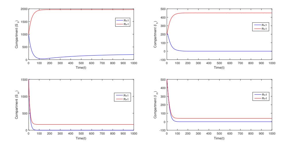
Figure 1: Time series of the compartments for R<1 and R>1. The parameters are: \(\beta_h=8.24\times 10^{-2},\ \beta_m=0.1648,\ \lambda_h=8.471\times 10^{-3},\ \lambda_m=2\times 10^{-4},\ \mu_h=3.9\times 10^{-5},\ \mu_m=7.14\times 10^{-2},\ u=5\times 10^{-4},\ \alpha_1=5,\ \alpha_2=5,\ r_h=0.1429,\ \gamma_h=2.74\times 10^{-3},\ d=1.452\times 10^{-4}\) and \(\beta_h=8.24\times 10^{-2},\ \beta_m=0.1648,\ \lambda_h=1,\ \lambda_m=15,\ \mu_h=3.9\times 10^{-5}, u=5\times 10^{-4},\ \mu_m=7.14\times 10^{-2},\ \alpha_1=5,\ \alpha_2=5,\ r_h=0.1429,\ \gamma_h=2.74\times 10^{-3},\ d=1.452\times 10^{-4}.\)
In order to examine the effect of saturated incidence rate over the compartments, Figure 2 have been generated by varying the values of \(\alpha_1\) and \(\alpha_2\). The dynamics of the compartments with and without saturation effect have been shown by taking \(\alpha_1 = \alpha_2 = 0\) and \(\alpha_1 = \alpha_2 = 5\) respectively. The other parameters of Table 2 are unchanged. The figure 2 depicts there is a considerable difference in the dynamics of the compartments by changing the unsaturated effect into saturated. For unsaturated phenomenon, the susceptible vanishes and the infected fluctuates within very short time whereas in case of saturation effect, the results are more realistic.
A constant treatment function have been used in the model (2) which represents the maximum treatment capacity after the outbreak of the disease. However, this capacity varies from city to city as well as from country to country. It is well known that the more adequate treatment gives the less infection. To see the effect Figure 3 has been generated for different values of u and the other parameters of Table 2 remain same. From Figure 2 it can be seen that the increased value of u decreases the index of the figure of infected population.
3.5. Sensitivity Analysis
Sensitivity analysis reveals the effect of each parameter for disease transmission. Usually in epidemiological diseases error involves in data collection and in the prediction of parameter values. In order to determine the robustness of model predictions to parameter values, the sensitivity analysis have often been used [13]. The estimation of the normalized forward sensitivity index of a variable to a parameter has been carried out by the ratio of the relative change in the variable to the relative change in the parameter. Partial derivatives may alternatively use for sensitivity index when the variable is a differentiable function of the parameter [42], [43]. Since the reproduction number is a threshold quantity for epidemic model, the sensitivity analysis have been used to determine the parameters that have a high or low effect on R.
Definition 3.1. [13], [42] The normalized forward sensitivity index of a variable R that depends differentiably on a parameter p is defined by
\[\psi_p^R = \frac{\partial R}{\partial p} \times \frac{p}{R}.\tag{12}\]
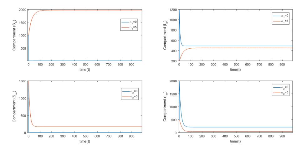
Figure 2: Effect of saturation incidence rate. The other parameters are: \(\beta_h = 8.24 \times 10^{-2}, \ \beta_m = 0.1648, \ \lambda_h = 1, \ \lambda_m = 15, \ \mu_h = 3.9 \times 10^{-5}, u = 5 \times 10^{-4}, \ \mu_m = 7.14 \times 10^{-2}, \ \alpha_1 = 5, \ \alpha_2 = 5, \ r_h = 0.1429, \ \gamma_h = 2.74 \times 10^{-3}, \ d = 1.452 \times 10^{-4}.\)
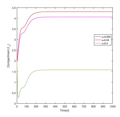
Figure 3: Effect of treatment function over Infected human. Others parameters are: \(\beta_h = 8.24 \times 10^{-2}, \ \beta_m = 0.1648, \ \lambda_h = 0.01, \ \lambda_m = 0.15, \ \mu_h = 3.9 \times 10^{-5}, \ \mu_m = 7.14 \times 10^{-2}, \ \alpha_1 = 5, \ \alpha_2 = 5, \ r_h = 0.1429, \ \gamma_h = 2.74 \times 10^{-3}, \ d = 1.452 \times 10^{-4}.\)
The expression of R from (3) is used to derive the analytical expressions for sensitivity incidence of R with respect to the parameter that comprise it. It is noted that the sensitivity index could be constant and do not depend on any parameter. It could also be complex expressions depending on several parameters of the model. The sensitivity incidences of R with respect to the model parameters is given by,
\[\psi_{\beta_h}^R = \psi_{\beta_m}^R = \psi_{\lambda_h}^R = \psi_{\lambda_m}^R = \frac{1}{2}, \psi_{\mu_m}^R = -1, \psi_d^R = -\frac{d}{2(r_h + \mu_h + d)}, \psi_{r_h}^R = -\frac{r_h}{2(r_h + \mu_h + d)},\]\[\psi_{\mu_h}^R = -\frac{r_h + 2\mu_h + d}{2(r_h + \mu_h + d)}.\]
Using the parameter values from Table 2, the sensitivity indices of R with respect to the parameters is given in Table 3.
| Parameter | Sensitivity indices |
|---|---|
| 0.5 | |
| \(\beta_m\) | 0.5 |
| \(\lambda_h\) | 0.5 |
| \(\lambda_m\) | 0.5 |
| \(\mu_h\) | -0.50013628 |
| \(\mu_m\) | -1 |
| d | -0.00050739 |
| \(r_h\) | -0.49935632 |
Table 3: Sensitivity indices of R to the model parameters.
From Table 3, it is found that \(\beta_h\), \(\beta_m\), \(\lambda_h\), and \(\lambda_m\) have the positive sensitivity index and the value is 0.5. That means increase (or decrease) any of these parameters by 10% will increase (or decrease) the reproduction number (R) by 5%. On the other hand the parameters \(\mu_h\), \(\mu_m\), d, and \(r_h\) have negative sensitivity indices. This indicates the increase (or decrease) of any of these parameters will decrease (or increase) R. It is found that the sensitivity index of \(\mu_m\) is -1. This represents the increase (or decrease) of \(\mu_m\) by 10 % will decrease (or increase) R by 10 %. From the analysis, it is concluded that the most sensitive parameter is the death rate of mosquito \((\mu_m)\). To validate the result, Figure 4 have been drawn by varying the value of \(\mu_m\) and keeping the other parameters from Table 2 as same. From Figure 4, it is observed that the increased value of \(\mu_m\) decreases the saturation level of the infected human. This suggests that the strategies can be used to increase the death rate of mosquito in order to decrease the reproduction number as well as the infection.
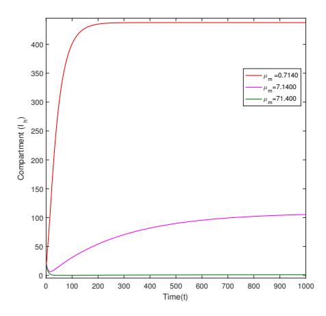
Figure 4: Effect of \(I_h\) of the variation of \(\mu_m\). The other parameters are: \(\beta_h = 8.24 \times 10^{-2}\), \(\beta_m = 0.1648\), \(\lambda_h = 1\), \(\lambda_m = 15\), \(\mu_h = 3.9 \times 10^{-5}\), \(\mu_h = 5 \times 10^{-4}\), \(\mu_h = 5\), \(\mu_h = 5\), \(\mu_h = 1.429\), \(\mu_h = 1.429\), \(\mu_h = 1.429\), \(\mu_h = 1.429\), \(\mu_h = 1.429\), \(\mu_h = 1.429\), \(\mu_h = 1.429\), \(\mu_h = 1.429\), \(\mu_h = 1.429\), \(\mu_h = 1.429\), \(\mu_h = 1.429\), \(\mu_h = 1.429\), \(\mu_h = 1.429\), \(\mu_h = 1.429\), \(\mu_h = 1.429\), \(\mu_h = 1.429\), \(\mu_h = 1.429\), \(\mu_h = 1.429\), \(\mu_h = 1.429\), \(\mu_h = 1.429\), \(\mu_h = 1.429\), \(\mu_h = 1.429\), \(\mu_h = 1.429\), \(\mu_h = 1.429\), \(\mu_h = 1.429\), \(\mu_h = 1.429\), \(\mu_h = 1.429\), \(\mu_h = 1.429\), \(\mu_h = 1.429\), \(\mu_h = 1.429\), \(\mu_h = 1.429\), \(\mu_h = 1.429\), \(\mu_h = 1.429\), \(\mu_h = 1.429\), \(\mu_h = 1.429\), \(\mu_h = 1.429\), \(\mu_h = 1.429\), \(\mu_h = 1.429\), \(\mu_h = 1.429\), \(\mu_h = 1.429\), \(\mu_h = 1.429\), \(\mu_h = 1.429\), \(\mu_h = 1.429\), \(\mu_h = 1.429\), \(\mu_h = 1.429\), \(\mu_h = 1.429\), \(\mu_h = 1.429\), \(\mu_h = 1.429\), \(\mu_h = 1.429\), \(\mu_h = 1.429\), \(\mu_h = 1.429\), \(\mu_h = 1.429\), \(\mu_h = 1.429\), \(\mu_h = 1.429\), \(\mu_h = 1.429\), \(\mu_h = 1.429\), \(\mu_h = 1.429\), \(\mu_h = 1.429\), \(\mu_h = 1.429\), \(\mu_h = 1.429\), \(\mu_h = 1.429\), \(\mu_h = 1.429\), \(\mu_h = 1.429\), \(\mu_h = 1.429\), \(\mu_h = 1.429\), \(\mu_h = 1.429\), \(\mu_h = 1.429\), \(\mu_h = 1.429\), \(\mu_h = 1.429\), \(\mu_h = 1.429\), \(\mu_h = 1.429\), \(\mu_h = 1.429\), \(\mu_h = 1.429\), \(\mu_h = 1.429\), \(\mu_h = 1.429\), \(\mu_h = 1.429\), \(\mu_h = 1.429\), \(\mu_h = 1.429\), \(\mu_h = 1.429\), \(\mu_h = 1.429\), \(\mu_h = 1.429\), \(\mu_h = 1.429\), \(\mu_h = 1.429\), \(\mu_h = 1.429\), \(\mu_h = 1.429\), \(\mu_h = 1.429\), \(\mu_h = 1.429\), \(\mu_h = 1.429\), \(\mu_h = 1.429\), \(\mu_h = 1.429\), \(\mu_h = 1.429\), \(\mu_h = 1.429\), \(\mu_h = 1.429\), \(\mu_h = 1.429\), \(\mu_h = 1.429\), \(\mu_h = 1.429\), \(\mu_h = 1.429\), \(\mu_h = 1.429\), \(\mu_h = 1.429\), \(\mu_h = 1.429\), \(\mu_h = 1.429\), \(\mu_h = 1.429\), \(\mu_h = 1.429\), \(\mu_h = 1.429\), \(\mu_h = 1.429\), \(\mu_h = 1.429\), \(\mu_h = 1.429\), \(\mu_h = 1.429\), \(\mu_h = 1.429\), \(\mu_h = 1.429\), \(\mu_h = 1.429\), \(\mu_h = 1.429\), \(\mu_h = 1.429\), \(\mu_h = 1.429\), \(\mu_h = 1.429\), \(\mu_h = 1.429\), \(\mu_h = 1.429\), \(\mu_h = 1.429\), \(\mu_h = 1.429\), \(\mu_h = 1.429\), \(\mu_h = 1.429\), \(\mu_h = 1.429\), \(\mu_h =\)
4. CONCLUSION
A simple and relevant mathematical model has been formulated and analyzed that describes the transmission of dengue with saturated incidence rate for both human and vector populations. A constant treatment function has been used to investigate the effect of treatment capacity in case of an epidemic scenario. The basic quantities such as disease free equilibrium, endemic equilibrium, and basic reproduction number have been calculated. It is found that the endemic equilibrium point exists when the reproduction number is greater than one. Moreover, the cases for unique and more than one endemic equilibrium have been pointed out. The local stability of the equilibrium points has been established based on the root of Jacobian matrix, and Lyapunov functions are constructed for the establishment of global stability. It is noted that the asymptotic
stability for both disease free and endemic equilibrium points depends on reproduction number. The disease free equilibrium point is globally asymptotically stable when R ≤ 1. On the other hand, the endemic equilibrium point is globally asymptotically stable when R > 1. Value of the parameters for infection rate and disease related death rate has been estimated based on real data collected from several health institutions of Bangladesh. From the particulars of data, it is noticeable that the outbreak of dengue in Bangladesh is becoming epidemic day by day. Time series of the compartments have been generated by developing MATLAB code, and the simulations exhibit that the disease dies out for R < 1 and hang on for R > 1. Besides, it is observed that the treatment function has an intensive effect on the infected human. The increased rate of treatment function reduces the infection. This indicates the sufficient treatment facility is needed to be ensured to disappear the endemic equilibrium and to get rid of the disease, otherwise the infection scenario will become out of control. From the sensitivity analysis, the highest sensitivity index is found for the mosquito death rate µm and this parameter has considered as the most sensitive parameter. It is found that the increased rate of µm gives the maximum fall of reproduction number and no other parameter has that much effect to reduce the infection. However, if the complete eradication of the infection is desirable in the community then the mosquito death rates should be increased. It is high time for the policy makers of Bangladesh to take appropriate steps to increase mosquito death rate and to ensure adequate treatment facility otherwise the situation can be out of control and a large number of death can be involved by this disease.
AVAILABILITY OF DATA
The data presented in Table-1 have been collected from Institute of Epidemiology Disease Control and Research (IEDCR), and from Directorate General of Health Services, Bangladesh.
ACKNOWLEDGEMENT
The authors are grateful to the anonymous reviewers for their careful reading, suggestions and comments that helped to improve the quality of the manuscript. This work was supported by SUST research center (grant number: PS/2017/24), Shahjalal University of Science and Technology, Sylhet-3114, Bangladesh.