

1. INTRODUCTION
Most countries in the world have been affected by various infectious diseases, such as, influenza, rubella, and the Coronavirus disease (COVID-19). The later has been affecting 2 international conveyances and 213 countries (territories) and with the total reported number of cases is at least 36,122,499 in the world [1]. Recently a number of researchers have reported their studies relating to this disease spread [2] [3]. Obviously, an accurate method for simulating and predicting the behaviour of the pandemic infectious disease spread is needed.
A number of authors have used SEIR models in the simulation of the infectious disease spread. Qureshi [4] proposed the use of the SEIR model to study periodic dynamics of rubella epidemic in Pakistan. Carcione et al. [5] studied a deterministic COVID-19 SEIR model. Arcede et al. [6] accounted for a COVID-19 SEIR-type model including both the symptomatic and asymptomatic cases. He et al. [7] also reported the dynamics of COVID-19 using the SEIR modeling. In addition to these studies, properties of SEIR-type models have been reported by Wei and Xue [8], Sun and Hsieh [9], Hou and Teng [10], Zhao et al. [11], as well as Jansen and Twizell [12].
With the important role of SEIR models in the simulation of the infectious disease spread, accurate methods are indeed needed to solve the models. This is because until now, the general exact analytical solution to SEIR models are not available. Therefore, approximate approach is a way to solve the models. Our work shall focus on a SEIR model of infectious disease involving constant vaccination strategy, where the population size is varying.
We have three contributions in this paper. The first is to provide successive approximation and variational iteration methods to obtain analytical approximate solutions to the SEIR model. The second is to prove that the successive approximation and variational iteration methods are identical when they are used to solve the
| Table 1: Variables and parameters in the SEIR model involving vaccination strategy. | ||
|---|---|---|
| Notation | Description |
|---|---|
| t | the time variable |
| N(t) | the total population in the system at time t |
| S(t) | the number of individuals of the susceptible subpopulation at time t |
| E(t) | the number of individuals of the exposed subpopulation at time t |
| I(t) | the number of individuals of the infected subpopulation at time t |
| R(t) | the number of individuals of the recovered subpopulation at time t |
| α | the incidence coefficient of horizontal transmission |
| β | the infection rate of the exposed individuals |
| γ | the recovery rate of the infected individuals |
| µ | the natural birth rate, which is assumed to be equal to the natural death rate of each group of the population |
| ν | the vaccination rate of the susceptible individuals, where the vaccination is assumed to be effective perfectly |
| σ | the death rate due to infection |
SEIR model with particular values of Lagrange multipliers in the variational iteration formulation. Third, we propose a new multistage-analytical method for solving the SEIR model very accurately in a large domain of time.
The rest of this paper is arranged as follows. We recall the SEIR model in Section 2. Proposed solving methods for the SEIR model are provided in Section 3. Then, we present results and discussion in Section 4. Finally, Section 5 shall conclude the paper.
2. SEIR MODEL
We recall the SEIR mathematical model for infectious disease spread in this section. This SEIR model involving constant vaccination is given by [13] [14] [15] [16]
\[\frac{dS(t)}{dt} = \mu N(t) - (\alpha I(t) + \mu + \nu)S(t),\tag{1}\]
\[\frac{dE(t)}{dt} = \alpha I(t)S(t) - (\beta + \mu)E(t), \tag{2}\]
\[\frac{dI(t)}{dt} = \beta E(t) - (\sigma + \gamma + \mu)I(t), \tag{3}\]
\[\frac{dR(t)}{dt} = \gamma I(t) + \nu S(t) - \mu R(t), \tag{4}\]
where descriptions of all variables and parameters are listed in Table 1. All variables are assumed to be non-negative and all parameters are assumed to be positive. Here, we also assume that the natural birth rate equals to the natural death rate of each group of the population. The initial conditions at time t = t0 are
\[S(t_0) = S_0, \quad E(t_0) = E_0, \quad I(t_0) = I_0, \quad R(t_0) = R_0,\] (5)
where S0, E0, I0, R0 are known constants. Here, the time domain is t ≥ t0 for a known constant t0. The S, E, I, R groups are all disjoint, where the total population N at time t is
\[N(t) = S(t) + E(t) + I(t) + R(t).\] (6)
Notice that the SEIR model is more complex than the SIR model [17] [18], because in the SEIR model we have variable E(t) in addition to variables S(t), I(t), and R(t).
The SEIR model (1)-(4) admits that the total population N is varying with time t. We can observe it by adding Equations (1)-(4) to result in dN/dt = −σI. If σ = 0, then the total population N is constant; but this is not the case for some infectious diseases, such as COVID-19. Readers interested in the local and global analyses of the SEIR model are referred to the work of Sun and Hsieh [9]. We focus on solving the SEIR model (1)-(4) in this paper.
Explicit exact solutions to SEIR Model (1)-(4) are not available until this paper is written. In addition, infectious disease is currently an important issue in the world. Therefore, in this paper, we aim to provide
explicit analytical solutions to SEIR Model (1)-(4) using analytical approach of approximation for simulation of the infectious disease spread. Moreover, we aim to propose a multistage-analytical method for solving the SEIR model, so that the obtained solution approximates the exact solution very accurately for a large time domain.
3. ANALYTICAL SOLVING METHODS
This section is devoted to provide three approaches for solving SEIR Model (1)-(4), namely, successive approximation, variational iteration, and multistage-analytical methods. Relation between successive approximation and variational iteration methods shall also be provided in this section.
3.1. Successive approximation method (SAM)
Our successive approximation method (SAM) takes the idea of Picard's successive approximations for solving initial value problems [19].
Picard's successive approximations are constructed as follows. Suppose that we have problem
\[\frac{dy(x)}{dx} = f(x,y) \tag{7}\]
with initial condition
\[y(x_0) = y_0, (8)\]
in which all involved functions are assumed to be smooth. With initial condition (8), the solution to problem (7) is
\[y(x) = y_0 + \int_{x_0}^x f(x, y) dx.\] (9)
Picard's successive approximations for solving problem (7)-(8) take the form
\[y_{n+1}(x) = y_0 + \int_{x_0}^x f(\xi, y_n(\xi)) d\xi,\] (10)
where n = 0, 1, 2, .... As n −→ ∞, we obtain [19]
\[\lim_{n \to \infty} y_n(x) = y(x),\tag{11}\] which is the solution to problem (7)-(8).
Considering that the total population is given by Equation (6), we can rewrite Equation (1) as
\[\frac{dS}{dt} = -\nu S + \mu E + \mu I + \mu R - \alpha I S. \tag{12}\]
For solving problem (1)-(5), SAM has the form
\[S_{n+1}(t) = S_0 + \int_{t_0}^t \left[ -\nu S_n(\tau) + \mu E_n(\tau) + \mu I_n(\tau) + \mu R_n(\tau) - \alpha S_n(\tau) I_n(\tau) \right] d\tau, \tag{13}\]
\[E_{n+1}(t) = E_0 + \int_{t_0}^t \left[ \alpha S_n(\tau) I_n(\tau) - (\beta + \mu) E_n(\tau) \right] d\tau, \tag{14}\]
\[I_{n+1}(t) = I_0 + \int_{t_0}^t \left[ \beta E_n(\tau) - (\sigma + \gamma + \mu) I_n(\tau) \right] d\tau, \tag{15}\]
\[R_{n+1}(t) = R_0 + \int_{t_0}^t \left[ \gamma I_n(\tau) + \nu S_n(\tau) - \mu R_n(\tau) \right] d\tau, \tag{16}\]
where n = 0, 1, 2, ....
3.2. Variational iteration method (VIM)
In this subsection, we provide a variational iteration method (VIM) for solving Equations (1)-(4). We adopt the variational iteration formulation of He [20] [21]. In our VIM formulation, we use Equation (12) rather than Equation (1), as also the case for SAM in the previous subsection.
The correction functionals of Equations (12) and (2)-(4) with initial conditions (5) are
\[S_{n+1}(t) = S_n(t) + \int_{t_0}^t \lambda_1(\tau) \left[ \frac{dS_n}{d\tau} + \nu S_n - \mu \tilde{E}_n - \mu \tilde{I}_n - \mu \tilde{R}_n + \alpha \tilde{I}_n \tilde{S}_n \right] d\tau, \tag{17}\]
\[E_{n+1}(t) = E_n(t) + \int_{t_0}^t \lambda_2(\tau) \left[ \frac{dE_n}{d\tau} - \alpha \tilde{I}_n \tilde{S}_n + (\beta + \mu) E_n \right] d\tau, \tag{18}\]
\[I_{n+1}(t) = I_n(t) + \int_{t_0}^t \lambda_3(\tau) \left[ \frac{dI_n}{d\tau} - \beta \tilde{E}_n + (\sigma + \gamma + \mu)I_n \right] d\tau, \tag{19}\]
\[R_{n+1}(t) = R_n(t) + \int_{t_0}^t \lambda_4(\tau) \left[ \frac{dR_n}{d\tau} - \gamma \tilde{I}_n - \nu \tilde{S}_n + \mu R_n \right] d\tau, \tag{20}\]
where \(\lambda_1(\tau)\), \(\lambda_2(\tau)\), \(\lambda_3(\tau)\), and \(\lambda_4(\tau)\) are Lagrange multipliers and n=0,1,2,.... Here \(\tilde{S}_n\), \(\tilde{E}_n\), \(\tilde{I}_n\), and \(\tilde{R}_n\) are restricted variations, which means that they behave like constants, that is, \(\delta \tilde{S}_n=0\), \(\delta \tilde{E}_n=0\), \(\delta \tilde{I}_n=0\), and \(\delta \tilde{R}_n=0\).
Operating variations to Equations (17)-(20), we have
\[\delta S_{n+1}(t) = \delta S_n(t) + \delta \int_{t_0}^t \lambda_1(\tau) \left[ \frac{dS_n}{d\tau} + \nu S_n \right] d\tau, \tag{21}\]
\[\delta E_{n+1}(t) = \delta E_n(t) + \delta \int_{t_0}^t \lambda_2(\tau) \left[ \frac{dE_n}{d\tau} + (\beta + \mu)E_n \right] d\tau, \tag{22}\]
\[\delta I_{n+1}(t) = \delta I_n(t) + \delta \int_{t_0}^t \lambda_3(\tau) \left[ \frac{dI_n}{d\tau} + (\sigma + \gamma + \mu)I_n \right] d\tau, \tag{23}\]
\[\delta R_{n+1}(t) = \delta R_n(t) + \delta \int_{t_0}^t \lambda_4(\tau) \left[ \frac{dR_n}{d\tau} + \mu R_n \right] d\tau.\] (24)
Applying integration by parts, we rewrite equations (21)-(24) as
\[\delta S_{n+1}(t) = \delta \left[ (\lambda_1(t) + 1) S_n(t) \right] - \delta \int_{t_0}^t \left[ \lambda_1'(\tau) - \nu \lambda_1(\tau) \right] S_n(\tau) d\tau, \tag{25}\]
\[\delta E_{n+1}(t) = \delta \left[ (\lambda_2(t) + 1) E_n(t) \right] - \delta \int_{t_0}^t \left[ \lambda_2'(\tau) - (\beta + \mu) \lambda_2(\tau) \right] E_n(\tau) d\tau, \tag{26}\]
\[\delta I_{n+1}(t) = \delta \left[ (\lambda_3(t) + 1)I_n(t) \right] - \delta \int_{t_0}^t \left[ \lambda_3'(\tau) - (\sigma + \gamma + \mu)\lambda_3(\tau) \right] I_n(\tau) d\tau, \tag{27}\]
\[\delta R_{n+1}(t) = \delta \left[ (\lambda_4(t) + 1) R_n(t) \right] - \delta \int_{t_0}^t \left[ \lambda_4'(\tau) - \mu \lambda_4(\tau) \right] R_n(\tau) d\tau. \tag{28}\]
Equations (25)-(28) lead to the following stationary conditions
\[\lambda_1(t) + 1 = 0, \quad \lambda_1'(\tau) - \nu \lambda_1(\tau) = 0,\] (29)
\[\lambda_2(t) + 1 = 0, \quad \lambda_2'(\tau) - (\beta + \mu)\lambda_2(\tau) = 0,\] (30)
\[\lambda_3(t) + 1 = 0, \quad \lambda_3'(\tau) - (\sigma + \gamma + \mu)\lambda_3(\tau) = 0,\] (31)
\[\lambda_4(t) + 1 = 0, \quad \lambda_4'(\tau) - \mu \lambda_4(\tau) = 0.\] (32)
Based on Equations (29)-(32), we obtain the following Lagrange multipliers
\[\lambda_1(\tau) = -\exp\left(\nu(\tau - t)\right),\tag{33}\]
\[\lambda_2(\tau) = -\exp\left((\beta + \mu)(\tau - t)\right),\tag{34}\]
\[\lambda_3(\tau) = -\exp\left((\sigma + \gamma + \mu)(\tau - t)\right),\tag{35}\]
\[\lambda_4(\tau) = -\exp\left(\mu(\tau - t)\right). \tag{36}\]
Finally, the variational iteration method (VIM) for solving (1)-(4) with initial conditions (5) is obtained as follows
\[S_{n+1}(t) = S_n(t) - \int_{t_0}^t \exp(\nu(\tau - t))\] \[\left[ \frac{dS_n}{d\tau} + \nu S_n - \mu E_n - \mu I_n - \mu R_n + \alpha I_n S_n \right] d\tau, \tag{37}\]
\[E_{n+1}(t) = E_n(t) - \int_{t_0}^t \exp\left((\beta + \mu)(\tau - t)\right) \left[\frac{dE_n}{d\tau} - \alpha I_n S_n + (\beta + \mu) E_n\right] d\tau,\] (38)
\[I_{n+1}(t) = I_n(t) - \int_{t_0}^t \exp\left((\sigma + \gamma + \mu)(\tau - t)\right) \left[\frac{dI_n}{d\tau} - \beta E_n + (\sigma + \gamma + \mu)I_n\right] d\tau,\] (39)
\[R_{n+1}(t) = R_n(t) - \int_{t_0}^t \exp(\mu(\tau - t)) \left[ \frac{dR_n}{d\tau} - \gamma I_n - \nu S_n + \mu R_n \right] d\tau, \tag{40}\]
where n = 0, 1, 2, ....
3.3. Relation between SAM and VIM
In this subsection, we prove the relation between SAM and VIM.
Theorem 3.1. Suppose that time t is close enough to t0 (that is, τ is close enough to t). If the Lagrange multipliers in the correction functionals (17)-(20) are all approximated by −1, that is,
\[\lambda_1(\tau) = -\exp\left(\nu(\tau - t)\right) \approx -1,\tag{41}\]
\[\lambda_2(\tau) = -\exp\left((\beta + \mu)(\tau - t)\right) \approx -1,\tag{42}\]
\[\lambda_3(\tau) = -\exp\left((\sigma + \gamma + \mu)(\tau - t)\right) \approx -1,\tag{43}\]
\[\lambda_4(\tau) = -\exp\left(\mu(\tau - t)\right) \approx -1,\tag{44}\] then the resulted VIM for solving the SEIR model (1)-(4) is identical with SAM for solving the same model. Proof: If we take approximate Lagrange multipliers
\[\lambda_1(\tau) = \lambda_2(\tau) = \lambda_3(\tau) = \lambda_4(\tau) = -1,\tag{45}\]
we have a new VIM for solving problem (1)-(5) in the following form
\[S_{n+1}(t) = S_n(t) - \int_{t_0}^t \left[ \frac{dS_n}{d\tau} + \nu S_n - \mu E_n - \mu I_n - \mu R_n + \alpha I_n S_n \right] d\tau, \tag{46}\]
\[E_{n+1}(t) = E_n(t) - \int_{t_0}^t \left[ \frac{dE_n}{d\tau} - \alpha I_n S_n + (\beta + \mu) E_n \right] d\tau, \tag{47}\]
\[I_{n+1}(t) = I_n(t) - \int_{t_0}^t \left[ \frac{dI_n}{d\tau} - \beta E_n + (\sigma + \gamma + \mu) I_n \right] d\tau, \tag{48}\]
\[R_{n+1}(t) = R_n(t) - \int_{t_0}^t \left[ \frac{dR_n}{d\tau} - \gamma I_n - \nu S_n + \mu R_n \right] d\tau.\] (49)
We note that
\[\int_{t_0}^t \left[ \frac{dS_n}{d\tau} \right] d\tau = S_n(t) - S_n(t_0), \tag{50}\]
\[\int_{t_0}^{t} \left[ \frac{dE_n}{d\tau} \right] d\tau = E_n(t) - E_n(t_0), \tag{51}\]
\[\int_{t_0}^{t} \left[ \frac{dI_n}{d\tau} \right] d\tau = I_n(t) - I_n(t_0), \tag{52}\]
\[\int_{t_0}^{t} \left[ \frac{dR_n}{d\tau} \right] d\tau = R_n(t) - R_n(t_0). \tag{53}\]
In addition, for all n, Equations (46)-(49) guarantee that
\[S_n(t_0) = S_0, \quad E_n(t_0) = E_0, \quad I_n(t_0) = I_0, \quad R_n(t_0) = R_0.\] (54)
Taking Equations (50)-(54) into account, we simplify Equations (46)-(49) as
\[S_{n+1}(t) = S_0 + \int_{t_0}^t \left[ -\nu S_n + \mu E_n + \mu I_n + \mu R_n - \alpha I_n S_n \right] d\tau, \tag{55}\]
\[E_{n+1}(t) = E_0 + \int_{t_0}^t \left[ \alpha I_n S_n - (\beta + \mu) E_n \right] d\tau, \tag{56}\]
\[I_{n+1}(t) = I_0 + \int_{t_0}^t \left[ \beta E_n - (\sigma + \gamma + \mu) I_n \right] d\tau, \tag{57}\]
\[R_{n+1}(t) = R_0 + \int_{t_0}^t \left[ \gamma I_n + \nu S_n - \mu R_n \right] d\tau.\] (58)
We observe that Equations (55)-(58) are identical with Equations (13)-(16). The proof is complete. From Theorem 3.1, VIM (37)-(40) and SAM (13)-(16) are identical when all Lagrange multipliers in the VIM formulation are approximated to be −1, which is the first term in the Taylor series expansion of the Lagrange multipliers. These approximate Lagrange multipliers are valid as long as time t is close enough to t0. With this knowledge, we propose a new multistage-analytical method in the next subsection.
3.4. Multistage-analytical method
Generally, SAM (13)-(16) and VIM (37)-(40) are accurate only for small time domain, and we shall show in the next section that this statement is true. Therefore, it is a good idea to implement SAM and VIM piecewisely, that is, in a multistage way. By piecewise or multistage we mean that the time domain \(I = [t_0, T]\) is subdivided into finite number of subdomains \(I_j = [t_{j-1}, t_j]\) having the same width, where j = 1, 2, 3, ..., J. We denote \(\Delta t = t_j - t_{j-1}\) for all j. The multistage-analytical method implements SAM or VIM on these subdomains \(I_j\) consecutively.
We observe that the calculation of SAM is simpler that that of VIM. In VIM, we need to differentiate some functions and then do integration. This is expensive in terms of computation. Due to this fact, we choose to use SAM in the multistage-analytical method. Therefore, our multistage-analytical method is called the multistage successive approximation method (MSAM).
MSAM works as follows. We denote \(S_{n,j}(t)\) the solution for S(t) at the nth iteration of SAM on the jth subdomain. Notations \(E_{n,j}(t)\), \(I_{n,j}(t)\), and \(R_{n,j}(t)\) have analogous meaning for E(t), I(t), and R(t), respectively. We denote K the maximum number of iterations of SAM in the MSAM evolution, which is set initially.
For j = 1, 2, 3, ..., J we implement SAM: so, for n = 0, 1, 2, ..., K - 1 we have
\[S_{n+1,j}(t) = S_{K,j-1}(t_{j-1}) + \int_{t_{j-1}}^{t} \left[ -\nu S_{n,j}(\tau) + \mu E_{n,j}(\tau) + \mu I_{n,j}(\tau) + \mu R_{n,j}(\tau) - \alpha S_{n,j}(\tau) I_{n,j}(\tau) \right] d\tau,\] (59)
\[E_{n+1,j}(t) = E_{K,j-1}(t_{j-1}) + \int_{t_{j-1}}^{t} \left[ \alpha S_{n,j}(\tau) I_{n,j}(\tau) - (\beta + \mu) E_{n,j}(\tau) \right] d\tau, \tag{60}\]
\[I_{n+1,j}(t) = I_{K,j-1}(t_{j-1}) + \int_{t_{j-1}}^{t} \left[\beta E_{n,j}(\tau) - (\sigma + \gamma + \mu) I_{n,j}(\tau)\right] d\tau, \tag{61}\]
\[R_{n+1,j}(t) = R_{K,j-1}(t_{j-1}) + \int_{t_{j-1}}^{t} \left[ \gamma I_{n,j}(\tau) + \nu S_{n,j}(\tau) - \mu R_{n,j}(\tau) \right] d\tau.\] (62)
We observe that if we take K=1, MSAM is identical with Euler's method. Taking higher value of K leads to higher order of accuracy, as we shall see in the next section.
4. RESULTS AND DISCUSSION
We simulate the spread of an infectious disease in this section. Parameter values are recorded in Table 2, where some of them are adopted from the work of Harir et al. [22]. All simulations are to be compared with available reference solutions, but they are not exact solutions, as the exact solutions are not available. Error is defined as the average of relative errors of MSAM solutions with respect to the reference solutions. The reference solutions are computed using the ode45 function available in the MATLAB software with the relative tolerance (RelTol) is \(2.22045 \times 10^{-14}\) and the absolute tolerance (AbsTol) is \(10^{-15}\).
We note that for our simulations, as written in Table 2, the initial population is \(N(0) = 270 \times 10^6\), the initial number of exposed individuals is \(E(0) = 38 \times 10^3\), the initial number of infected individuals is \(I(0) = 23 \times 10^3\), and the initial number of recovered individuals is \(R(0) = 13 \times 10^3\). We assume that the rest belongs to the susceptible group. This means that almost all people in the system are susceptible initially; this is our assumption for the simulations.
Solutions to the SEIR model on SAM are as follows. The initialisations of SAM are
\[S_0 = 270 \times 10^6 - E_0 - I_0 - R_0, \quad E_0 = 38 \times 10^3, \quad I_0 = 23 \times 10^3, \quad R_0 = 13 \times 10^3.\] (63)
The first iteration solutions of SAM are
\[S_1(t) = -\frac{3297798167587717}{1073741824}t + 269926000, (64)\]
\[E_1(t) = \frac{3174924693756969}{8589934592}t + 38000, (65)\]
| Notation | Value | Description |
|---|---|---|
| N(0) | 270 × 106 | the total population in the system at time t = 0 |
| S(0) | N(0) − E(0) − I(0) − R(0) | the number of individuals of the susceptible subpopulation at time t = 0 |
| E(0) | 38 × 103 | the number of individuals of the exposed subpopulation at time t = 0 |
| I(0) | 23 × 103 | the number of individuals of the infected subpopulation at time t = 0 |
| R(0) | 13 × 103 | the number of individuals of the recovered subpopulation at time t = 0 |
| α | 6 × 10⁻⁸ | the incidence coefficient of horizontal transmission |
| β | 7 × 10⁻² | the infection rate of the exposed individuals |
| γ | 5 × 10⁻² | the recovery rate of the infected individuals |
| µ | 6 × 10⁻³ | the natural birth rate, which is assumed to be equal to the natural death rate |
| ν | 7 × 10⁻⁷ | the vaccination rate of the susceptible individuals |
| σ | 1 × 10⁻² | the death rate due to infection |
Table 2: Parameter values for SEIR model simulation, where N = S + E + I + R.
\[I_1(t) = \frac{6034049004685861}{4398046511104}t + 23000, (66)\]
\[R_1(t) = 2700332 t + 13000. (67)\]
These SAM iterations can be continued.
Solutions to the SEIR model on VIM are as follows. The initialisations of VIM are the same as those of SAM, as given by Equations (63). The first iteration solutions of VIM are
\[S_1(t) = \frac{11331148222878377973682565575}{36893488147419103232} \exp\left(-\frac{t}{100}\right) - \frac{1372636541198129114681733575}{36893488147419103232},\] (68)
\[E_1(t) = -\frac{6818098863474499429259163875}{1401952549601925922816} \exp\left(-\frac{19 t}{250}\right) + \frac{6871373060359372614326171875}{1401952549601925922816},\] (69)
\[I_{1}(t) = -\frac{98861858892773116760}{4035275706439791} \exp\left(-\frac{4035275706439791 t}{72057594037927936}\right) + \frac{191673200140888309760}{4035275706439791},\] \[(70)\]
\[R_1(t) = -\frac{1350166000}{3} \exp\left(-\frac{3t}{500}\right) + \frac{1350205000}{3}.\] (71)
These VIM iterations can be continued.
Simulation results using SAM and VIM are shown in Figure 1 for S(t), Figure 2 for E(t), Figure 3 for I(t), and Figure 4 for R(t). In this simulation we use three iterations for each of SAM and VIM evolutions. We observe that as time t gets larger, SAM and VIM solutions are inaccurate. We see at time t = 2 in these figures (especially in Figures 1-3), that there exist obvious discrepancies between SAM and VIM solutions in comparison with the reference solutions.
In contrast, the solutions produced using our proposed multistage-analytical method are very accurate, as shown in Figure 5. In this simulation, we consider the time domain [0, 60] with ∆t = 0.25. In order to obtain MSAM solutions, on each subdomain, we evolve SAM up to two iterations. We observe from Figure 5 that MSAM solutions graphically coincide with the reference solutions for the whole large domain of time.
We obtain that the smaller the time step ∆t leads to the smaller the errors of MSAM solutions. This can be observed from Tables 3-8. Tables 3-4 show that one SAM iteration in the MSAM evolution leads to that MSAM is of the first order of accuracy; we infer this from the results that as ∆t approaches 0, the order
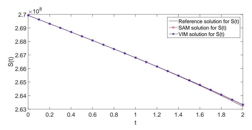
Figure 1: Reference, SAM, and VIM solutions for S(t) on interval [0,2]. Here SAM and VIM solutions are generated at their third iterations. Reference, SAM, and VIM solutions almost coincide each other, but only for small size of time interval.
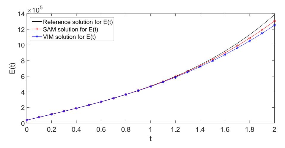
Figure 2: Reference, SAM, and VIM solutions for E(t) on interval [0,2]. Here SAM and VIM solutions are generated at their third iterations. Reference, SAM, and VIM solutions almost coincide each other, but only for small size of time interval.
Table 3: Errors and verification of Order of Covergence (OC) when MSAM uses 1 iteration of SAM for \(S_{1,j}(t)\) and \(E_{1,j}(t)\) on the interval [0,60].
| \(\Delta t\) | Error of \(S_{1,j}(t)\) | OC of \(S_{1,j}(t)\) | Error of \(E_{1,j}(t)\) | OC of \(E_{1,j}(t)\) |
|---|---|---|---|---|
| 0.25 | 1.16513E-01 | _ | 5.70500E-02 | _ |
| 0.20 | 8.56992E-02 | 1.38 | 4.70855E-02 | 0.86 |
| 0.10 | 3.67650E-02 | 1.22 | 2.51902E-02 | 0.90 |
| 0.05 | 1.71527E-02 | 1.10 | 1.30663E-02 | 0.95 |
| 0.01 | 3.25673E-03 | 1.03 | 2.69527E-03 | 0.98 |
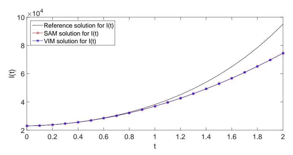
Figure 3: Reference, SAM, and VIM solutions for I(t) on interval [0, 2]. Here SAM and VIM solutions are generated at their third iterations. Reference, SAM, and VIM solutions almost coincide each other, but only for small size of time interval.
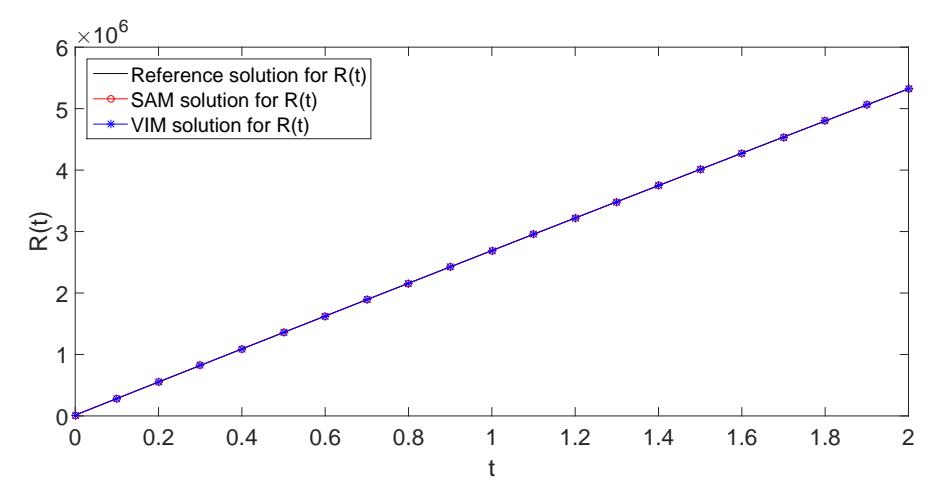
Figure 4: Reference, SAM, and VIM solutions for R(t) on interval [0, 2]. Here SAM and VIM solutions are generated at their third iterations. Reference, SAM, and VIM solutions almost coincide each other, but only for small size of time interval.
Table 4: Errors and verification of Order of Covergence (OC) when MSAM uses 1 iteration of SAM for I1,j (t) and R1,j (t) on the interval [0, 60].
| ∆t | Error of I1,j (t) | OC of I1,j (t) | Error of R1,j (t) | OC of R1,j (t) |
|---|---|---|---|---|
| 0.25 | 6.78644E-02 | – | 1.77054E-02 | – |
| 0.20 | 5.63537E-02 | 0.83 | 1.43347E-02 | 0.95 |
| 0.10 | 3.05349E-02 | 0.88 | 7.34519E-03 | 0.96 |
| 0.05 | 1.59446E-02 | 0.94 | 3.71920E-03 | 0.98 |
| 0.01 | 3.30720E-03 | 0.98 | 7.51527E-04 | 0.99 |
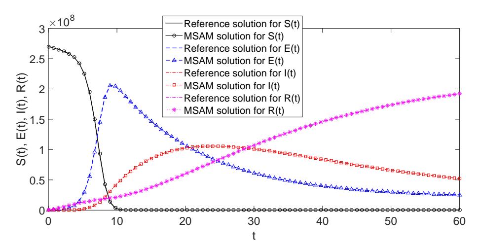
Figure 5: Reference and MSAM solutions for S(t), E(t), I(t), R(t) on interval [0,60]. Here MSAM solutions are generated using two iterations on each subdomain. MSAM solutions graphically coincide with the reference solutions for the whole large size of time domain.
Table 5: Errors and verification of Order of Covergence (OC) when MSAM uses 2 iterations of SAM for \(S_{2,j}(t)\) and \(E_{2,j}(t)\) on the interval [0, 60].
| \(\Delta t\) | Error of \(S_{2,j}(t)\) | OC of \(S_{2,j}(t)\) | Error of \(E_{2,j}(t)\) | OC of \(E_{2,j}(t)\) |
|---|---|---|---|---|
| 0.25 | 1.15973E-02 | _ | 5.02941E-03 | _ |
| 0.20 | 7.00158E-03 | 2.26 | 3.33385E-03 | 1.84 |
| 0.10 | 1.64632E-03 | 2.09 | 8.94285E-04 | 1.90 |
| 0.05 | 4.07249E-04 | 2.02 | 2.31577E-04 | 1.95 |
| 0.01 | 1.62767E-05 | 2.00 | 9.52694E-06 | 1.98 |
Table 6: Errors and verification of Order of Covergence (OC) when MSAM uses 2 iterations of SAM for \(I_{2,j}(t)\) and \(R_{2,j}(t)\) on the interval [0,60].
| \(\Delta t\) | Error of \(I_{2,j}(t)\) | OC of \(I_{2,j}(t)\) | Error of \(R_{2,j}(t)\) | OC of \(R_{2,j}(t)\) |
|---|---|---|---|---|
| 0.25 | 5.37407E-03 | _ | 1.16799E-03 | _ |
| 0.20 | 3.57265E-03 | 1.83 | 7.72759E-04 | 1.85 |
| 0.10 | 9.63224E-04 | 1.89 | 2.06895E-04 | 1.90 |
| 0.05 | 2.49987E-04 | 1.95 | 5.35714E-05 | 1.95 |
| 0.01 | 1.03010E-05 | 1.98 | 2.20479E-06 | 1.98 |
Table 7: Errors and verification of Order of Covergence (OC) when MSAM uses 3 iterations of SAM for \(S_{3,j}(t)\) and \(E_{3,j}(t)\) on the interval [0,60].
| \(\Delta t\) | Error of \(S_{3,j}(t)\) | OC of \(S_{3,j}(t)\) | Error of \(E_{3,j}(t)\) | OC of \(E_{3,j}(t)\) |
|---|---|---|---|---|
| 0.25 | 5.64572E-04 | _ | 2.83822E-04 | _ |
| 0.20 | 2.68405E-04 | 3.33 | 1.50926E-04 | 2.83 |
| 0.10 | 2.90895E-05 | 3.21 | 2.03673E-05 | 2.89 |
| 0.05 | 3.40242E-06 | 3.10 | 2.64669E-06 | 2.94 |
| 0.01 | 2.59415E-08 | 3.03 | 2.18440E-08 | 2.98 |
Table 8: Errors and verification of Order of Covergence (OC) when MSAM uses 3 iterations of SAM for I3,j (t) and R3,j (t) on the interval [0, 60].
| ∆t | Error of I3,j (t) | OC of I3,j (t) | Error of R3,j (t) | OC of R3,j (t) |
|---|---|---|---|---|
| 0.25 | 3.28712E-04 | – | 6.92957E-05 | – |
| 0.20 | 1.74686E-04 | 2.83 | 3.68060E-05 | 2.84 |
| 0.10 | 2.35314E-05 | 2.89 | 4.95241E-06 | 2.89 |
| 0.05 | 3.05401E-06 | 2.95 | 6.42444E-07 | 2.95 |
| 0.01 | 2.51796E-08 | 2.98 | 5.29482E-09 | 2.98 |
of convergence tends to 1. Tables 5-6 show that two SAM iterations in the MSAM evolution leads to that MSAM is of the second order of accuracy; we see this from the results that as ∆t approaches 0, the order of convergence tends to 2. Furthermore, Tables 7-8 indicate that three SAM iterations in the MSAM evolution leads to that MSAM is of the third order of accuracy; because as ∆t approaches 0, the order of convergence tends to 3. The higher the number of SAM iterations in the MSAM evolution results in the higher the order of convergence (the order of accuracy) of the MSAM solutions.
5. CONCLUSION
We have presented three contributions in this paper. First, successive approximation and variational iteration methods are provided for solving the SEIR model in analytical approximate ways. As the second contribution, we prove that both the variational iteration and successive approximation methods are identical in the case of some particular values of Lagrange multipliers in the variational iteration formulation of the model. Third, we have proposed a new multistage-analytical method for solving the SEIR model. Our proposed multistage-analytical method solves the SEIR model very accurately for a large domain of time. Error of the multistage-analytical solution decreases and tends to zero, as the time step is taken smaller (approaches zero). In addition, higher order of accuracy of the proposed multistage-analytical method can be achieved simply by taking more number of successive approximation iterations in the multistage evolution.
ACKNOWLEDGEMENTS
This research was financially supported by an LPPM-USD grant with contract number 035/Penel./LPPM-USD/V/2020 of Sanata Dharma University year 2020.