

1. Introduction
The Coronavirus disease 2019, also known as COVID-19, is an infectious disease caused by a new type of coronavirus (SARS-CoV-2) known to have originated in December 2019 in the city of Wuhan in China [1]. COVID-19 is a human-to-human transmitted disease, transmitted through direct contact with infected individuals or objects that had been contaminated with the virus on the surfaces [2]. The symptoms of COVID-19 resemble those of ordinary flu but could lead to death as a consequence of the difficulty in breathing for patients in advanced stages. Till now, there is no medicine to cure infected individuals [3].
Policymakers have been forced to use many types of interventions to control the rapid spread of COVID-19. These include physical/social distancing, use of face masks, quarantine, hospitalization, rapid testing, and vaccination [2]. Due to the limited availability of vaccines in the community, the most popular and effective way to control the spread of COVID-19 is to prevent infection through non-pharmaceutical interventions such as physical distancing, use of medical masks, quarantine, use of disinfectants, contact tracing, etc. [3]. Among the strategies implemented the most to minimize the risk of infection are social distancing and the use of medical masks. The implementation of these strategies can be more effective if the level of social awareness is high in the population concerned [4].
<sup>2</sup> Department of Mathematics, University of Raparin, Ranya, Kurdistan Region, Iraq
<sup>3</sup> Department of Pure and Applied Mathematics, University of Haripur, KP, Pakistan
*Corresponding author
Received June \(4^{th}\), 2021, Revised June \(27^{th}\), 2021, Accepted for publication July \(1^{st}\), 2021. Copyright ©2021 Published by Indonesian Biomathematical Society, e-ISSN: 2549-2896, DOI:10.5614/cbms.2021.4.1.5
Since early 2020, many mathematical models have been introduced by many authors from all over the world to understand the dynamics of COVID-19's spread among different populations. Many approaches have been used by these authors such as ordinary differential equations [5], [6], [7], [8], [9], partial differential equation [11], statistics [12], [13], [14], artificial intelligence and optimal control approaches [15], [16]. Their research has covered several important factors such as the impact of vaccination [10], social distancing [1], [17], hospitalization [18], contact tracing [18], [19], and social awareness [2], [3], [4], [17]. From the previously mentioned literature, several important results are presented. Firstly, the role of social distancing is significant in reducing the spread of COVID-19 in various countries, even in some cases better than vaccination intervention. Secondly, the role of hospitalization in reducing the number of COVID-19 infections is not as significant as social distancing. Even so, hospitalization is still needed to accelerate the rate of recovery of cases detected by COVID-19 and to avoid further death rate induced by COVID-19. Another result is that contact tracing coupled with the isolation of detected cases has a significant effect in reducing the number of new COVID-19 infections. Finally, the role of media campaigns is important to increase social awareness. It is needed as a companion to other interventions such as vaccination and social distancing because the potential target of social awareness is wider than other interventions. Hence, we can conclude that the massive implementation of mentioned interventions will reduce the spread of COVID-19. However, this kind of policy will entail costly interventions. Hence, it is important to determine the best strategy to combat the spread of COVID-19. One option is to use the strategy of optimal control problem. Furthermore, to determine the best strategy, cost-effectiveness analysis can also be carried out to analyze this problem.
Thus, this article aims to analyze the impact of human awareness and rapid testing as efforts to reduce the spread of COVID-19. To test the validation of our model, we have used the incidence data from the city of Jakarta in Indonesia pertaining to the initial phase of the disease. We conducted a mathematical analysis to understand the qualitative behavior of the model, which is related to the existence and local stability criteria of the equilibrium points and how these depend on the size of the basic reproduction number. Moreover, bifurcation analysis of the model was conducted using the center manifold approach. An optimal control problem is conducted to see how a time-dependent intervention could reduce the number of infected individuals while keeping the cost of intervention low. A cost-effectiveness analysis is carried out to determine the best possible scenario to be implemented in the field.
This article is organized as follows. In Section 2, we construct our model using several assumptions. We analyze our proposed model in Section 4, followed by elasticity and autonomous simulation in Section 5. The characterization of the optimal control problem is given in Section 6. The numerical experiments of the optimal control problem and cost-effectiveness analysis are detailed in Section 7. Finally, we present the conclusions in Section 8.
2. MODEL CONSTRUCTION
In this section, we construct the model for the spread of COVID-19 carefully, using government campaign interventions to increase awareness and rapid tests as a pair of possible interventions. To start with, based on their health and their awareness status, the population was categorized as follows: susceptible without awareness (Su), susceptible with awareness (Sa), exposed (E), undetected infected individuals (Iu), detected infected individuals (Id), and recovered individuals (R). For a detailed description of each of these categories; see Table 1, and Figure 1 for the transmission process of our model.
The assumptions of our model are as follows.
- 1) The population is closed, and the migration is neglected.
- 2) Each individual in the population is homogeneous in the sense of how they respond to this disease.
- 3) All new-born are assumed to be susceptible and unaware of COVID-19.
- 4) Both susceptible without awareness (Su) and susceptible with awareness (Sa) can be infected with COVID-19, with a successful transmission rate of β1 and β2, respectively. Due to awareness of Sa, we assume that β2 < β1.
- 5) Due to hospitalization/forced self-quarantine, only undetected infected individuals can transmit the virus, while the individuals whose infection has been detected cannot. In the proposed model, we assume that hospitalization/quarantine perfectly isolates from the infected individual. With this assumption, we neglect a "local" infection in the hospital for the hospital worker.
- 6) Infected compartment (Id, Iu) may die due to COVID-19 with the same rate of ξ.
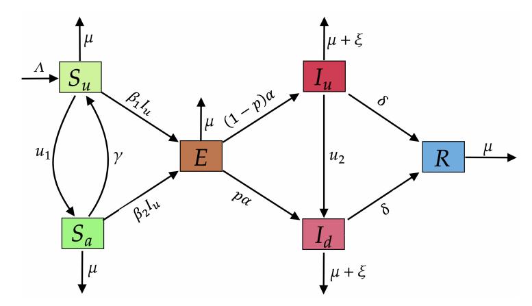
Figure 1: Transmission diagram for COVID-19 with social awareness and rapid test.
Table 1: Description of model variables given in system (1).
| Variable | Description |
|---|---|
| \(S_u\) | Susceptible without awareness \((S_u)\) is a population that is not infected and does not care about the presence of COVID-19. Usually, individuals belonging to this category roam around freely, without observing the precautions such as wearing masks and maintaining social distance. |
| \(S_a\) | Susceptible with awareness \((S_a)\) is a population that is not infected and cares about the presence of COVID-19. Individuals falling in this category usually do not roam freely, without ruling out the possibility of doing so. Even if they roam freely, they adhere to the suggested health protocols. |
| E | Exposed \((E)\) are residents who have contracted COVID-19, but did not transmit the disease to others. This is usually called the latent phase. |
| \(I_u\) | Infected but not detected \((I_u)\) is the population infected with COVID-19 that can transmit the disease to other individuals. They are individuals who roam so they are not detected as infected with COVID-19. |
| \(I_d\) | Infected and detected (\(I_d\)) is the population infected with COVID-19 that has been detected. However, as their infection was detected, they had to be self-isolated or taken to the hospital for treatment. Therefore, they cannot infect other people. |
| R | Recovered \((R)\) is the population that has recovered from the COVID-19 disease. |
- 7) Due to a media campaigns to increase social awareness about the dangers of COVID-19, we assume that there is a transition rate of \(u_1\) from \(S_u\) to \(S_a\). However, the awareness of individuals is not for lifetime. Hence, there is a dropout rate from \(S_a\) to \(S_u\), namely as \(\gamma\).
- 8) Rapid test intervention \((u_2)\) conducted to detect infected individuals.
Based on the transmission diagram in Figure 1 and the above assumptions, the COVID-19 model with social awareness and rapid test can be expressed in the nonlinear system of differential equations stated below.
\[\frac{dS_u}{dt} = \Lambda - \beta_1 S_u I_u - u_1 S_u + \gamma S_a - \mu S_u,\] \[\frac{dS_a}{dt} = u_1 S_u - \gamma S_a - \beta_2 S_a I_u - \mu S_a,\] \[\frac{dE}{dt} = \beta_1 S_u I_u + \beta_2 S_a I_u - \alpha E - \mu E,\] \[\frac{dI_u}{dt} = (1 - p)\alpha E - \delta I_u - \xi I_u - u_2 I_u - \mu I_u,\] \[\frac{dI_d}{dt} = p\alpha E - \delta I_d - \xi I_d + u_2 I_u - \mu I_d\] \[\frac{dR}{dt} = \delta (I_u + I_d) - \mu R,\] (1)
completed with a non-negative initial condition at t = 0; see Table 2 for the description of each parameter.
[10]
Having used a similar approach in our previous work [1], [2], it is clear that our model always has a positive solution for all situations t > 0 as long as the initial condition is non-negative, and positively invariant in the region of
\[\Omega = \left\{ (S_u, S_a, E, I_u, I_d, R) \in \mathbb{R}^6_+ | 0 \le S_u + S_a + E + I_u + I_d + R \le \frac{\Lambda}{\mu} \right\}.\]
Value Parameter Description Source Λ Human recruitment rate \(/(70 \times 365)\)[4] Proportion of individuals who move from the exposed to the infected and 0.4 [20], [21] pdetected compartment 1 - pProportion of individuals who move from the exposed to the infected but not [20], [21] detected group Rate of government intervention to raise social awareness estimated \(u_1\)Rate of government intervention to conduct rapid tests estimated \(u_2\)1/5.1[22], [23], [24], [25] Incubation rate \(\beta_1\)Rate of transmission of unaware susceptible individuals \(1.85 \times 10\)fitted \(8.3\times10^{-8}\)Rate of transmission of aware susceptible individuals fitted Drop-out rate from aware to unaware susceptible group 0.10.1 [2] \(1/(70 \times 365)\)Natural death rate [26] μ
Table 2: Model parameters with their descriptions and estimated values
3. PARAMETER ESTIMATION
To validate our model, we estimate our infection rate \((\beta_1, \beta_2)\) in system (1) using incidence data from the city of Jakarta, during the early phases of COVID-19 spread in the city (March 3- April 10, 2020). We intend to minimize the Euclidian distance between \(I_d\) from incidence data and the simulation results from system (1), using the best fit parameter of \(\beta_1\) and \(\beta_2\). This task read as minimizing the following function
\[SE = \sum_{n=1}^{m} \left( I_d^{\text{data}} - I_u^{\text{solution}} \right)^2,\] where \(I_d^{\text{data}}\) present incidence data, and \(I_d^{\text{solution}}\) present the solution of \(I_d\) form system (1) using the best fit parameter of \(\beta_1\) and \(\beta_2\). These parameters were estimated using the "Isqnonlin" built-in function in MATLAB. The initial guess for initial conditions and estimated parameters were chosen at the first iteration, and will be updated in each next iteration until convergence criteria achieved \((|SE_{(i+1)^{th}}|_{\text{iteration}} - SE_{(i)^{th}}|_{\text{iteration}}| < 10^{-2})\).
Our aim is to capture the initial COVID-19 parameter value in Jakarta where interventions have not yet been implemented. Hence, we assume that in the early spread of COVID-19, the effort from the government to conduct rapid tests and media campaigns to develop community awareness were not yet significantly implemented. Hence, we assume that \(u_1 = u_2 = 0\) in this period of simulation (March 3 - April 10, 2020). The result given for the curve fitting can be seen in Figure 2, and the parameters are given in Table 1.
4. MODEL ANALYSIS
This section explores the qualitative behavior of our proposed model in system (1) regarding the existence and local stability of all possible equilibrium points and how these criteria related to the basic reproduction number of the model.
4.1. Disease Free-Equilibrium (DFE) and the Basic Reproduction Number
Death rate due to COVID-19
DFE point is a condition in which the disease outbreak in a population will decrease over time. This means that for \(t \to \infty\), there are no more individuals classified as exposed (E), infected and detected \((I_d)\), and infected but undetected \((I_u)\). Taking the right-hand-side of system (1) as equal to zero and \(E = I_u = I_d = 0\), the model's DFE point is expressed as follows:
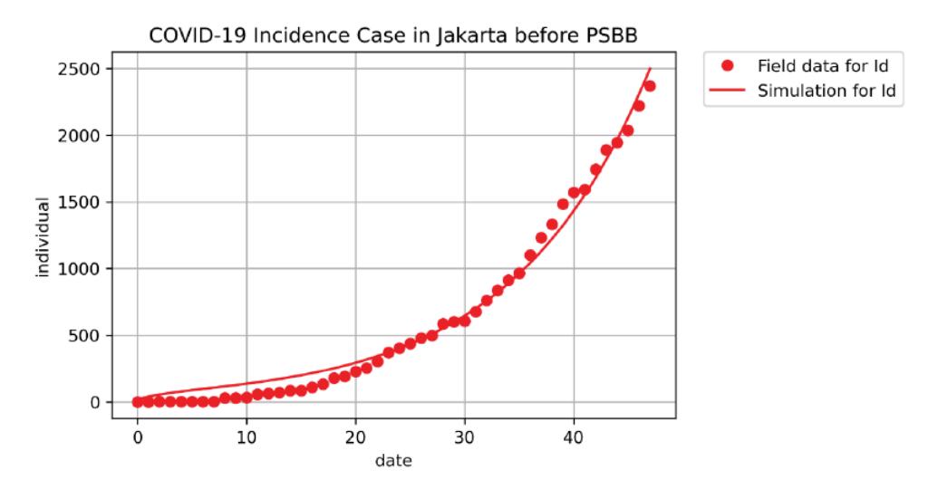
Figure 2: Curve fitting simulation results.
\[\text{DFE } = (S_u^0, S_a^0, E^0, I_u^0, I_d^0, R^0) = (\frac{(\gamma + \mu) \Lambda}{\mu \ (\gamma + \mu + u_1)}, \frac{u_1 \Lambda}{\mu \ (\gamma + \mu + u_1)}, 0, 0, 0, 0).\]
In many mathematical models, the local stability of DFE is related to a condition of the basic reproduction number \((\mathcal{R}_0)\) less than unity [2], [4], [27]. The basic reproduction number indicates the number of newly infected individuals caused by the primarily infected individual during the period of transmission to fully susceptible individuals. We calculate our respected \(\mathcal{R}_0\) of system (1) using the Next Generation Matrix (NGM) method. The idea to obtain the NGM method is by decomposition of the linearize matrix of the infected compartment at DFE. The obtained decomposition matrix contains a transmission component (T) and another transition component \((\Sigma)\). The transmission component is a component that contains the transmission parameters on the model. Furthermore, the transition component is a component that contains parameters that are displaced / change in the infection process. After the decomposition matrix is linearized using the Jacobian matrix, DFE is substituted into the matrix, leading to the following:
\[\mathbf{T} = \begin{bmatrix} 0 & \frac{u_1 \Lambda \beta_2}{\mu \left( \gamma + \mu + u_1 \right)} + \frac{(\gamma + \mu) \Lambda \beta_1}{\mu \left( \gamma + \mu + u_1 \right)} & 0 \\ 0 & 0 & 0 \\ 0 & 0 & 0 \end{bmatrix},\] and
\[\Sigma = \left[ \begin{array}{ccc} -\alpha - \mu & 0 & 0 \\ -\alpha \, p + \alpha & -\mu - \xi - \delta - u_2 & 0 \\ \alpha \, p & u_2 & -\mu - \xi - \delta \end{array} \right].\]
The basic reproduction number of the system (1) is taken from the spectral radius of respected NGM, where \(NGM = -\mathbf{E}_*^t \mathbf{T} \Sigma^{-1} \mathbf{E}_*\), where
\[\mathbf{E}_* = \left[ \begin{array}{c} 1 \\ 0 \\ 0 \end{array} \right].\]
Hence, the value of \(\mathcal{R}_0\) indicated by the following expression:
\[\mathcal{R}_{0} = \frac{\alpha \left(1 - p\right) \left(\gamma \beta_{1} + \beta_{1} \mu + u_{1} \beta_{2}\right) \Lambda}{\mu \left(\alpha + \mu\right) \left(\delta + \mu + \xi + u_{2}\right) \left(\gamma + \mu + u_{1}\right)}.\] (2)
With the expression of the basic reproduction number in equation (2), the local stability of DFE is furnished in the following theorem:
Theorem 4.1. The COVID-19 free equilibrium is locally stable if \(\mathcal{R}_0 < 1\), and unstable when \(\mathcal{R}_0 > 1\).
Proof: The Jacobian matrix of system (1) evaluated on DFE is given by
\[\mathbb{J} = \begin{bmatrix} -\mu - u_1 & \gamma & 0 & -\frac{(\gamma + \mu)\Lambda \beta_1}{\mu (\gamma + \mu + u_1)} & 0 & 0 \\\nu_1 & -\gamma - \mu & 0 & -\frac{u_1\Lambda \beta_2}{\mu (\gamma + \mu + u_1)} & 0 & 0 \\ 0 & 0 & -\alpha - \mu & \frac{u_1\Lambda \beta_2}{\mu (\gamma + \mu + u_1)} + \frac{(\gamma + \mu)\Lambda \beta_1}{\mu (\gamma + \mu + u_1)} & 0 & 0 \\ 0 & 0 & -\alpha p + \alpha & -\delta - \mu - \xi - u_2 & 0 & 0 \\ 0 & 0 & \alpha p & u_2 & -\delta - \mu - \xi & 0 \\ 0 & 0 & 0 & \delta & \delta & -\mu \end{bmatrix} .\] (3)
Matrix J has six eigenvalues, where four of them are explicitly negative, as indicated below:
\[-\mu, -\mu, -(\delta + \mu + \xi), \text{ and } -(u_1 + \gamma + \mu).\]
The two other eigenvalues are taken from the following quadratic polynomial:
\[a_2\lambda^2 + a_1\lambda + a_0 = 0.\] where
\[a_{2} = \mu (u_{1} + \gamma + \mu),\]
\[a_{1} = \mu (u_{2} + \alpha + \delta + 2 \mu + \xi) (u_{1} + \gamma + \mu),\]
\[a_{0} = \mu (\alpha + \mu) (u_{1} + \gamma + \mu) (u_{2} + \delta + \mu + \xi) (1 - R_{0}).\]
Based on the above equation, all the roots will have a negative real part if \(a_2, a_1\), and \(a_0 > 0\). Therefore, in this case, it must be \(\mathcal{R}_0 < 1\). On the other hand, if \(\mathcal{R}_0 > 1\), then we have one positive eigenvalues. Therefore, we have that DFE is unstable when \(\mathcal{R}_0 > 1\). Hence, the proof is completed.
The expression of \(\mathcal{R}_0\) on equation (2) is directly proportional to the term of (1-p) and inversely proportional to rapid test rates \(u_2\). Since 1-p describe a proportion of exposed individuals who progress to be undetected infected individuals, we can notice that more people can be detected (voluntarily go to the hospital or through rapid test) can reduce the basic reproduction number. More discussion on the impact of each parameters on \(\mathcal{R}_0\) will be discussed in section 5.
4.2. The Endemic Equilibrium Point
Another equilibrium point is the non-trivial one, called the endemic disease (EE) equilibrium point. Disease endemic equilibrium point (EE) is a condition where a disease in a population becomes an epidemic over time. The endemic equilibrium point of system (1) is given by
\[EE = (S_u^*, S_a^*, E^*, I_u^*, I_d^*, R^*),\] where
\[\begin{split} S_u^* &= \frac{\Lambda \; (I_u^* \beta_2 + \gamma + \mu)}{{I_u}^{*2} \beta_1 \beta_2 + \gamma \, I_u^* \beta_1 + \mu \, I_u^* \beta_1 + \mu \, I_u^* \beta_2 + I_u^* \beta_2 u_1 + \gamma \, \mu + \mu^2 + \mu \, u_1}, \\ S_a^* &= \frac{\Lambda \, u_1}{{I_u}^2 \beta_1 \beta_2 + \gamma \, I_u^* \beta_1 + \mu \, I_u^* \beta_1 + \mu \, I_u^* \beta_2 + I_u^* \beta_2 u_1 + \gamma \, \mu + \mu^2 + \mu \, u_1}, \\ E^* &= \frac{(\delta + \mu + \xi + u_2) \, I_u^*}{\alpha \; (1 - p)}, \\ I_u^* &= f(I_u), \\ I_d &= -\frac{I_u^* \, (\delta \, p + \mu \, p + p \xi + u_2)}{((\delta + \mu + \xi)(1 - p))}, \\ R &= \frac{\delta \; (\delta + \mu + \xi + u_2) \, I_u^*}{((\delta + \mu + \xi)(1 - p)) \, \mu}, \end{split}\] and \(I_u^*\) is taken from the positive root of the following polynomial:
\[f(I_u) := A_2 I_u^2 + A_1 I_u + A_0 = 0.\] with
\[A_{2} = \beta_{1}\beta_{2}(\alpha + \mu) (\delta + \mu + \xi + u_{2}),\] \[A_{1} = \alpha \beta_{1}\beta_{2} (p - 1) \Lambda + (\alpha + \mu) (\delta + \mu + \xi + u_{2}) (\gamma \beta_{1} + \beta_{1}\mu + \beta_{2}\mu + u_{1}\beta_{2}),\] \[A_{0} = \mu(\alpha + \mu)(\mu + \gamma + u_{1})(\delta + \mu + \xi + u_{2})(1 - \mathcal{R}_{0}).\]
It can be seen from the expression of all variables in EE that these equilibriums will be on \(\mathbb{R}^6_+\) if \(I^*_u > 0\). Hence, it is crucial to determine the criteria to guarantee the positivity of \(I^*_u\). It is trivial that since \(A_0 > 0 \iff \mathcal{R}_0 > 1\), we have exactly one real positive roots of \(f(I_u)\) when \(\mathcal{R}_0 > 1\). Hence, we have one endemic equilibrium when \(\mathcal{R}_0 > 1\). However, since \(f(I_u)\) is a second degree polynomial, it is possible to that \(f(I_u)\) have zero or two positive roots.
To analyze this, we can determine a condition of parameters such that \(\frac{A_0}{A_2}>0\), \(\frac{-A_1}{A_2}>0\), and \(A_1^2-4A_2A_0\geq 0\). However, this condition is difficult to show due to its complex expression of \(A_0\), \(A_1\), and \(A_2\). Hence, we will use a gradient analysis in a point of \(\mathcal{R}_0=1\), \(I_u=0\). The idea of this analysis is the following: As mentioned in Theorem 4.1, and analysis on previous paragraph regarding the existence of EE when \(\mathcal{R}_0>1\), we can see that \(\mathcal{R}_0=1\) has the potential to become a critical value which determines the existence and local stability of equilibrium points. Hence, it is important to analyze the gradient of \(f(I_u)\) at \(\mathcal{R}_0=1\). If the gradient is always positive, hence we never have any equilibrium points when \(\mathcal{R}_0<1\). On the other hand, if the gradient can be negative (under some conditions), then it is possible to have at least one endemic equilibrium point where \(\mathcal{R}_0<1\).
To do this, we rewrite each coefficient on \(f(I_u)\) as a function depends on \(\mathcal{R}_0\). Therefore, we redefine \(\beta_1\) as a function of \(\mathcal{R}_0\) as follows:
\[\beta_{1} = \frac{R_{0} (\alpha + \mu) (u_{1} + \gamma + \mu) (u_{2} + \delta + \mu + \xi) - \beta_{2} u_{1} \alpha (1 - p) \Lambda}{\alpha (1 - p) (\gamma + \mu) \Lambda}.\]
Substituting \(\beta_1\) into \(A_2\) and \(A_1\), then \(A_2\) and \(A_1\), are functions that contain \(\mathcal{R}_0\), as well as \(A_0\). This indicates that if \(\mathcal{R}_0 > 1\), system (1) will always have one endemic point. In addition, we investigate the possibility to have two endemic equilibriums (or none) if \(\mathcal{R}_0 < 1\).
Taking the partial derivative of \(I_u\) with respect to \(\mathcal{R}_0\) from the expression of \(f(I_u)\), we have
\[\frac{\partial A_2}{\partial \mathcal{R}_0} I^2 + A_2 2I \frac{\partial I}{\partial \mathcal{R}_0} + \frac{\partial A_1}{\partial \mathcal{R}_0} I + A_1 \frac{\partial I}{\partial \mathcal{R}_0} + \frac{\partial A_0}{\partial \mathcal{R}_0} = 0.\]
Substitute \((\mathcal{R}_0, I) = (1, 0)\) to the above equation and solve it with respect to \(\frac{\partial I}{\partial \mathcal{R}_0}\) yield:
\[\frac{\partial I}{\partial \mathcal{R}_0} = -\frac{\frac{\partial A_0}{\partial \mathcal{R}_0}}{A_1}.\]
Since,
\[\frac{\partial A_0}{\partial \mathcal{R}_0} = -\frac{\mu^2 (1-p)(\alpha+\mu)(u_1+\gamma+\mu)(u_2+\delta+\mu+\xi)}{(1-p)(\gamma+\mu)} - \frac{\gamma \mu (1-p)(\alpha+\mu)(u_1+\gamma+\mu)(u_2+\delta+\mu+\xi)}{(1-p)(\gamma+\mu)} < 0.\] and \(A_1>0\), we have that \(\frac{\partial I}{\partial \mathcal{R}_0}>0\). As mentioned before, since \(\frac{\partial I}{\partial \mathcal{R}_0}\) is always positive, then the gradient of \(f(I_u)\) is always tends to the right on \(\mathcal{R}_0=1\). This means that no positive roots when \(\mathcal{R}_0<1\). In other words, there is no endemic point when \(\mathcal{R}_0<1\). We express this result in the following theorem:
Theorem 4.2. System (1) has a unique endemic equilibrium if \(\mathcal{R}_0 > 1\), and no endemic equilibrium otherwise.
4.3. Bifurcation Analysis
We conduct a bifurcation analysis for system (1) using the Castillo-Song theorem [28]. The idea of this theorem is to show that there is a zero eigenvalue of system (1), while the other eigenvalues are negative at the DFE and \(\mathcal{R}_0 = 1\). The next approach is to analyze it using the center-manifold theory.
To simplify the notation, we rewrite \(S_u=x_1, S_a=x_2, E=x_3, I_u=x_4, I_d=x_5, R=x_6\) and then substitute it to system (1). Therefore, we have \(\frac{dx}{dt}=F(x)\) with \(F=(f_1,f_2,f_3,f_4,f_5,f_6)^T, X=(x_1,x_2,x_3,x_4,x_5,x_6)^T\) which are stated as follows:
\[f_{1} := \frac{dx_{1}}{dt} = \Lambda + \gamma x_{2} - \beta_{1} x_{1} x_{4} - u_{1} x_{1} - \mu x_{1},\] \[f_{2} := \frac{dx_{2}}{dt} = u_{1} x_{1} - \beta_{2} x_{2} x_{4} - \gamma x_{2} - \mu x_{2},\] \[f_{3} := \frac{dx_{3}}{dt} = \beta_{1} x_{1} x_{4} + \beta_{2} x_{2} x_{4} - \alpha x_{3} - \mu x_{3},\] \[f_{4} := \frac{dx_{4}}{dt} = (1 - p)\alpha x_{3} - u_{2} x_{4} - \delta x_{4} - \mu x_{4} - \xi x_{4},\] \[f_{5} := \frac{dx_{5}}{dt} = p\alpha x_{3} + u_{2} x_{4} - \delta x_{5} - \mu x_{5} - \xi x_{5},\] \[f_{6} := \frac{dx_{6}}{dt} = \delta x_{4} + \delta x_{5} - \mu x_{6}.\] \[(4)\]
Taking \(\beta_1\) as the bifurcation parameter with the expression is the same as in the previous section, we substitute it together with \(\mathcal{R}_0 = 1\) to the Jacobian matrix of the above system, we have:
\[\mathbb{J}_{1} = \begin{bmatrix} -\mu - u_{1} & \gamma & 0 & -\frac{(\gamma + \mu)\Lambda\beta^{*}}{\mu(\gamma + \mu + u_{1})} & 0 & 0 \\\nu_{1} & -\gamma - \mu & 0 & -\frac{u_{1}\Lambda\beta_{2}}{\mu(\gamma + \mu + u_{1})} & 0 & 0 \\ 0 & 0 & -\alpha - \mu & \frac{u_{1}\Lambda\beta_{2}}{\mu(\gamma + \mu + u_{1})} + \frac{(\gamma + \mu)\Lambda\beta^{*}}{\mu(\gamma + \mu + u_{1})} & 0 & 0 \\ 0 & 0 & -\alpha p + \alpha & -\delta - \mu - \xi - u_{2} & 0 & 0 \\ 0 & 0 & \alpha p & u_{2} & -\delta - \mu - \xi & 0 \\ 0 & 0 & 0 & \delta & \delta & -\mu \end{bmatrix}. \tag{5}\]
From the expression of \(\mathbb{J}_1\), we have a simple zero eigenvalue, while the others are negative (We do not show the expression of all negative eigenvalues due to their long expression). Thus, the center-manifold theory can be used to analyze the bifurcation of system (4).
Further, J1 has a right eigenvector denoted by w = (w1, w2, w3, w4, w5, w6) T given by
\[w_{1} = \frac{(\delta + \mu + \xi)\beta_{2}u_{1}(1 - p)\Lambda}{\delta(\gamma + \mu + u_{1})^{2}(\delta + \mu + \xi + u_{2})} - \frac{(\delta + \mu + \xi)(\alpha + \mu)(\gamma + \mu)}{\delta\alpha(\gamma + \mu + u_{1})} < 0,\] \[w_{2} = (\alpha\beta_{2}u_{1}(p - 1)\Lambda) - ((\alpha + \mu)(\gamma + \mu + u_{1})(\delta + \mu + \xi + u_{2})u_{1}) < 0,\] \[w_{3} = \frac{\mu(\delta + \mu + \xi)}{\alpha\delta} > 0,\] \[w_{4} = \frac{\mu(\delta + \mu + \xi(1 - p))}{\delta(\delta + \mu + \xi + u_{2})} > 0,\] \[w_{5} = \frac{\mu(\delta p + \mu p + \xi p + u_{2})}{\delta(\delta + \mu + \xi + u_{2})} > 0,\] \[w_{6} = 1.\] and a left eigenvector denoted by v = (v1, v2, v3, v4, v5, v6) T given by v1 = v2 = v5 = v6 = 0, v3 = α(1−p), and v4 = α + µ. Since v1 = v2 = v5 = v6 = 0, it is sufficient to calculate the partial derivatives of f3 and f4. Using the Castillo-Song theorem, we find the values of A and B as follows:
\[\mathcal{A} = \sum_{i,j=1}^{6} v_3 w_i w_j \frac{\partial^2 f_3}{\partial x_i \partial x_j} + \sum_{i,j=1}^{6} v_4 w_i w_j \frac{\partial^2 f_4}{\partial x_i \partial x_j},\] \[\mathcal{B} = \sum_{i,j=1}^{6} v_3 w_i \frac{\partial^2 f_3}{\partial x_i \partial \beta^*} + \sum_{i,j=1}^{6} v_4 w_i \frac{\partial^2 f_4}{\partial x_i \partial \beta^*}.\] where:
\[\mathcal{A} = 2 \frac{\left(1-p\right)\alpha\mu\left(\delta+\mu+\xi\left(1-p\right)\right)\beta_{1}}{\left(\delta+\mu+\xi+u_{2}\right)\delta} \left(\delta\left(-\frac{\left(\delta+\mu+\xi\right)\beta_{2}u_{1}\left(p-1\right)}{\left(\gamma+\mu+u_{1}\right)^{2}\left(\delta+\mu+\xi+u_{2}\right)\delta}\right)\Lambda + A_{0}\right),\] \[\mathcal{B} = \frac{\left(1-p\right)\alpha\left(\delta+\mu+\xi\left(1-p\right)\right)\left(\gamma+\mu\right)\Lambda}{\left(\delta+\mu+\xi+u_{2}\right)\delta\left(\gamma+\mu+u_{1}\right)}.\] with,
\[\begin{split} A_0 = &\delta\left(-\frac{(\delta+\mu+\xi)(\alpha\,\gamma+\alpha\,\mu+\gamma\,\mu+\mu^2)}{\delta\,\alpha\,(\gamma+\mu+u_1)}\right) + 2\left(\frac{(1-p)\alpha\,\mu\,(\delta+\mu+\xi\,(1-p))(\beta_2u_1\alpha\,(p-1)\Lambda}{(\delta+\mu+\xi+u_2)\delta}\right) \\ &- 2\left(\frac{(\alpha+\mu)(\delta+\mu+\xi+u_2)(\gamma+\mu+u_1)u_1)\beta_2}{(\delta+\mu+\xi+u_2)\delta}\right). \end{split}\]
It is found that A < 0 and B > 0. This indicates that system (6) forms a forward bifurcation at R0 = 1. Hence, we have the following theorem:
Theorem 4.3. The COVID-19 model in system (1) always exhibits a transcritical bifurcation at R0 = 1.
As a consequence of transcritical bifurcation phenomena that appear when R0 = 1, we can conclude that the endemic equilibrium is always locally asymptotically stable when R0 > 1, but close to one. It means that COVID-19 will always disappear from the community as long as we can keep the value of R0 at less than unity. To determine the best strategy to reduce the value of R0, we should understand which parameter is the most significant in determining the magnitude of R0. Hence, we proceed to the next section, where we discuss the sensitivity and elasticity of R0.
5. NUMERIC SIMULATION
5.1. The Elasticity of the Basic Reproduction Number
As mentioned earlier, it is important to determine which parameter is the most promising and can be changed to manipulate the size of R0. Hence, we conduct an elasticity analysis of R0 using the following formula :
\[\epsilon_{\mathcal{R}_0}^P = \frac{\partial \mathcal{R}_0}{\partial P} \times \frac{P}{\mathcal{R}_0},\] where P is any parameter on system (1). If the elasticity is negative, then increasing the parameter will reduce the magnitude of \(\mathcal{R}_0\). Using this formula, the local elasticity of each parameters in system (1) is expressed as follows:
\[\begin{split} \epsilon_{\mathcal{R}_0}^{\beta_1} &= \frac{\partial \mathcal{R}_0}{\partial \beta_1} \cdot \frac{\beta_1}{\mathcal{R}_0} = \frac{(\gamma + \mu)\beta_1}{\gamma \beta_1 + \mu \beta_1 + u_1 \beta_2} > 0 \\ \epsilon_{\mathcal{R}_0}^{\beta_2} &= \frac{\partial \mathcal{R}_0}{\partial \beta_2} \cdot \frac{\beta_2}{\mathcal{R}_0} = \frac{u_1 \beta_2}{\gamma \beta_1 + \mu \beta_1 + u_1 \beta_2} > 0 \\ \epsilon_{\mathcal{R}_0}^{\alpha} &= \frac{\partial \mathcal{R}_0}{\partial \alpha} \cdot \frac{\alpha}{\mathcal{R}_0} = \frac{\mu}{\alpha + \mu} > 0 \\ \epsilon_{\mathcal{R}_0}^{\gamma} &= \frac{\partial \mathcal{R}_0}{\partial \gamma} \cdot \frac{\gamma}{\mathcal{R}_0} = \frac{\mu}{\alpha + \mu} > 0 \\ \epsilon_{\mathcal{R}_0}^{p} &= \frac{\partial \mathcal{R}_0}{\partial p} \cdot \frac{p}{\mathcal{R}_0} = -\frac{p}{1 - p} < 0 \\ \epsilon_{\mathcal{R}_0}^{u_1} &= \frac{\partial \mathcal{R}_0}{\partial u_1} \cdot \frac{u_1}{\mathcal{R}_0} = -\frac{(\beta_1 - \beta_2)(\gamma + \mu)u_1}{(\gamma \beta_1 + \mu \beta_1 + u_1 \beta_2)(\gamma + \mu + u_1)} < 0 \\ \epsilon_{\mathcal{R}_0}^{u_2} &= \frac{\partial \mathcal{R}_0}{\partial u_2} \cdot \frac{u_2}{\mathcal{R}_0} = -\frac{u_2}{\delta + \mu + \xi + u_2} < 0 \\ \epsilon_{\mathcal{R}_0}^{\delta} &= \frac{\partial \mathcal{R}_0}{\partial \delta} \cdot \frac{\delta}{\mathcal{R}_0} = -\frac{\delta}{\delta + \mu + \xi + u_2} < 0 \\ \epsilon_{\mathcal{R}_0}^{\xi} &= \frac{\partial \mathcal{R}_0}{\partial \xi} \cdot \frac{\xi}{\mathcal{R}_0} = -\frac{\xi}{\delta + \mu + \xi + u_2} < 0 \\ \epsilon_{\mathcal{R}_0}^{\delta} &= \frac{\partial \mathcal{R}_0}{\partial \delta} \cdot \frac{\Lambda}{\mathcal{R}_0} = -\frac{\xi}{\delta + \mu + \xi + u_2} < 0 \\ \epsilon_{\mathcal{R}_0}^{\delta} &= \frac{\partial \mathcal{R}_0}{\partial \delta} \cdot \frac{\Lambda}{\mathcal{R}_0} = 1 > 0, \end{split}\] while \(\epsilon_{\mathcal{R}_0}^{\mu}\) is always negative, it has too long an expression to be shown in this article. So, by substituting the parameter values in Table 1, and supposing \(u_1 = u_2 = 0.1\), we get the following results:
\[\begin{array}{lll} \epsilon_{\mathcal{R}_0}^{\beta_1} &=& u_2 = 0.1, \\ \epsilon_{\mathcal{R}_0}^{\beta_2} &=& 0.691 \\ \epsilon_{\mathcal{R}_0}^{\beta_2} &=& 0.308 \\ \epsilon_{\mathcal{R}_0}^{\alpha} &=& 0.00019 \\ \epsilon_{\mathcal{R}_0}^{\gamma} &=& 0.1504 \\ \epsilon_{\mathcal{R}_0}^{\mu} &=& -0.6667 \\ \epsilon_{\mathcal{R}_0}^{\mu} &=& -1.0002 \\ \epsilon_{\mathcal{R}_0}^{\mu} &=& -0.1909 \\ \epsilon_{\mathcal{R}_0}^{u_2} &=& -0.3414 \\ \epsilon_{\mathcal{R}_0}^{\delta} &=& -0.4877 \\ \epsilon_{\mathcal{R}_0}^{\xi} &=& -0.1707 \\ \epsilon_{\mathcal{R}_0}^{\delta} &=& 1. \end{array}\]
Each value of the elasticity above presents a percentage value of \(\mathcal{R}_0\), whenever the parameter changed. For example, when \(\epsilon_{\mathcal{R}_0}^{\beta_1}=0.691\), it means that reducing \(\beta_1\) for 10% for its current value in Table 1, \(\mathcal{R}_0\) will be reduced to 6.91%. On the other hand, since \(\epsilon_{\mathcal{R}_0}^{u_1}=-0.1909\), increasing the magnitude of \(u_1\) for 10% will reduce the value of \(\mathcal{R}_0\) to 1.909%. To see which parameter is the most elastic to \(\mathcal{R}_0\); see Figure 3. It can be seen that \(\mu\) is the most elastic parameter to \(\mathcal{R}_0\). However, as we cannot change the value of \(\mu\), we may ignore this result. The reason is similar to the recruitment rate too (\(\Lambda\)). On the other hand, we can see that \(\beta_1\) is the most elastic changeable parameter. Hence, it is a very reasonable policy to enforce a "mini lockdown" in the city of Jakarta to control the spread of COVID-19 in the early period of the outereak. Interestingly, we can see that although \(u_1\) and \(u_2\) have a negative sign of elasticity, the value of \(|\epsilon_{\mathcal{R}_0}^{u_2}| > |\epsilon_{\mathcal{R}_0}^{u_1}|\). This means that rapid testing is more promising to control the spread of COVID-19 than media campaigns to increase
social awareness. However, we can not ignore the importance of social awareness in the case of COVID-19's transmission mechanism, as higher awareness in the community will reduce the possibility of people being infected by COVID-19. Thus, it is important to adopt the best combination strategy of these two types of control, which we shall discuss in the next section.
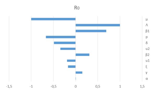
Figure 3: Tornado Diagram: Elasticity of R0
5.2. Autonomous Simulations
From the previous section, we can see the importance of choosing a proper value of u1 and u2 to determine the size of R0. Therefore, in this section, we conduct an autonomous simulation to see the impact of u1 and u2 on the dynamics of all infected individuals. We use the same value as stated in Table 1 and substitute it into the system (1). Before we show the autonomous simulation on the effect of u1 and u2, we should understand the impact of u1 and u2 on the size of R0. A dependency of R0 with respect to u1 and u2 is shown in Figure 4. It can be seen that when the parameters u1 and u2 are zero, the value of R0 is very high, i.e., it has high endemic potential. On the other hand, if u1 and u2 are large at the same time, then R0 will get smaller.
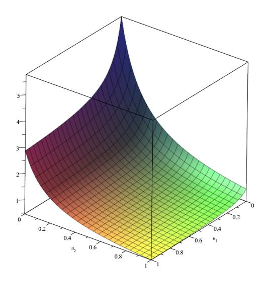
Figure 4: Sensitivity of u1 and u2 on R0
Next, we solve our set of ordinary differential equations using a Runge-Kutta numerical method, with the same set of parameters as in the previous figure. The results are shown in Figure 5.
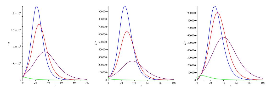
Figure 5: The trajectories of E, \(I_u\), and \(I_d\) for the different values \(u_1\) and \(u_2\) when \(u_1 = u_2 = 0.05, 0.1, 0.2\), and 0.8 for blue, red, purple, and green, respectively
In Figure 5, it can be seen that increasing the value of the \(u_1\) and \(u_2\) parameters will reduce the total number and the outbreak level of infected populations. Furthermore, the large intensity of \(u_1\) and \(u_2\) also delays the appearance of the outbreak. In other words, government intervention, by increasing social awareness through media campaigns \((u_1)\) and carrying out rapid tests \((u_2)\), succeeds in controlling the epidemic level of COVID-19. A higher intensity of both the controls will give a better result for eliminating COVID-19 from the population. However, we should notice that the high intensity of these interventions comes with higher cost of intervention. Hence, we should find a policy to combine these interventions. Using simple logic, these interventions should consider the number of infected individuals at each time. When the number of infected individuals starts increasing, the intensity of these interventions should be increased. On the other hand, when the number of infected individuals starts to decrease (or is a low number), then the intensity of the interventions should be low for the sake of budget economies.
6. OPTIMAL CONTROL CHARACTERIZATION
Based on the level of need in disease control efforts, various efforts were made by various parties concerned to provide cost-effective interventions to optimize control outcomes. In implementing this intervention, various costs must also be minimized: not only the costs of intervention but also indirect costs associated with the field implementation process with due regard to the number of people infected in the field. One option is to choose a time-dependent intervention for our model. Hence, we change a constant \(u_1\) and \(u_2\) in system (1) as a time-dependent variable, namely \(u_1(t)\) and \(u_2(t)\), respectively. Hence, system (1) now reads as follows:
\[\frac{dS_u}{dt} = \Lambda + \gamma S_a - \beta_1 S_u I_u - u_1(t) S_u - \mu S_u, \frac{dS_a}{dt} = u_1(t) S_u - \beta_2 S_a I_u - \gamma S_a - \mu S_a, \frac{dE}{dt} = \beta_1 S_u I_u + \beta_2 S_a I_u - \alpha E - \mu E, \frac{dI_u}{dt} = (1 - p)\alpha E - u_2(t) I_u - \delta I_u - \mu I_u - \xi I_u, \frac{dI_d}{dt} = p\alpha E + u_2(t) I_u - \delta I_d - \mu I_d - \xi I_d, \frac{dR}{dt} = \delta I_u + \delta I_d - \mu R.\] (6)
The aim of the optimal control problem in this article is to minimize the total number of infected individuals \((E, I_u, I_d)\) at as low a cost of intervention as possible \((u_1(t), u_2(t))\). Hence, we aim to minimize the following cost function:
\[J = \int_0^T (\varphi_1 u_1^2 + \varphi_2 u_2^2 + \omega_3 E + \omega_4 I_u + \omega_5 I_d) dt.\] (7)
To solve this, we first set the following Hamiltonian function:
\[H = \varphi_1 u_1^2 + \varphi_2 u_2^2 + \omega_3 E + \omega_4 I_u + \omega_5 I_d + \lambda_1 (\Lambda + \gamma S_a - \beta_1 S_u I_u - u_1 S_u - \mu S_u) + \lambda_2 (u_1 S_u - \beta_2 S_a I_u - \gamma S_a - \mu S_a) + \lambda_3 (\beta_1 S_u I_u + \beta_2 S_a I_u - \alpha E - \mu E t) + \lambda_4 (\alpha E - p \alpha E - u_2 I_u - \delta I_u - \mu I_u - \xi I_u) + \lambda_5 (p \alpha E + u_2 I_u - \delta I_d - \mu I_d - \xi I_d) + \lambda_6 (\delta I_u + \delta I_d - \mu R).\] where \(\lambda_i\) for i = 1, 2, 3, 4, 5, 6 is the adjoint variables.
Theorem 6.1. Given optimal control pairs \((u_1^*, u_2^*)\) and solutions \(S_u(t)\), \(S_a(t)\), E(t), \(I_u(t)\), \(I_d(t)\) and R(t) of the state system (7), there exist adjoint variables \(\lambda_i\) for i = 1, 2, 3, 4, 5, 6 which satisfy the following adjoint systems:
\[\dot{\lambda}_{1} = \lambda_{1}\beta_{1}I_{u} + \lambda_{1}u_{1} + \lambda_{1}\mu - \lambda_{2}u_{1} - \lambda_{3}\beta_{1}I_{u}\] \[\dot{\lambda}_{2} = -\lambda_{1}\gamma + \lambda_{2}\beta_{2}I_{u} + \lambda_{2}\gamma + \lambda_{2}\mu - \lambda_{3}\beta_{2}I_{u}\] \[\dot{\lambda}_{3} = -\omega_{3} + \lambda_{3}\alpha + \lambda_{3}\mu + \lambda_{4}p\alpha - \lambda_{4}\alpha - \lambda_{5}p\alpha\] \[\dot{\lambda}_{4} = -\omega_{4} + \lambda_{1}\beta_{1}S_{u} + \lambda_{2}\beta_{2}S_{a} - \lambda_{3}\beta_{1}S_{u} - \lambda_{3}\beta_{2}S_{a} + \lambda_{4}u_{2} + \lambda_{4}\delta + \lambda_{4}\mu + \lambda_{4}\xi - \lambda_{5}u_{2} - \lambda_{6}\delta\] \[\dot{\lambda}_{5} = -\omega_{5} + \lambda_{5}\delta + \lambda_{5}\mu + \lambda_{5}\xi - \lambda_{6}\delta\] \[\dot{\lambda}_{6} = \lambda_{6}\mu,\] (8)
with the terminal condition given by \(\lambda_i(T) = 0\) for i = 1, 2, 3, 4, 5, 6. Further, the optimal control pair is given by
\[u_{1}^{*}(t) = \min\left(u_{1}^{\max}, \max\left(u_{1}^{\min}, \frac{S_{u}(\lambda_{1} - \lambda_{2})}{2\omega_{1}}\right)\right),\] \[u_{2}^{*}(t) = \min\left(u_{2}^{\max}, \max\left(u_{2}^{\min}, \frac{I_{u}(\lambda_{4} - \lambda_{5})}{2\omega_{2}}\right)\right).\] (9)
Proof. Using the Pontryagin Maximum Principle [31], the adjoint system (8) is taken from the partial derivatives of the Hamiltonian H with respect to each state variable, as follows:
\[\dot{\lambda_1} = -\frac{\partial H}{\partial S_u}, \dot{\lambda_2} = -\frac{\partial H}{\partial S_a}, \ \dot{\lambda_3} = -\frac{\partial H}{\partial E}, \ \dot{\lambda_4} = -\frac{\partial H}{\partial I_u}, \ \dot{\lambda_5} = -\frac{\partial H}{\partial I_d}, \dot{\lambda_6} = -\frac{\partial H}{\partial R}.\] with the transversality condition \(\lambda_i(T) = 0\) for i = 1, 2, 3, 4, 5, 6. Taking the derivative of the Hamiltonian H with respect to \(u_1\) equal to zero, and solving it with respect to \(u_1\) yields
\[u_1^+ = \frac{S_u \left(\lambda_1 - \lambda_2\right)}{2\omega_1}.\]
Similarly, for \(u_2\) we have
\[u_2^+ = \frac{I_u(\lambda_4 - \lambda_5)}{2\omega_2}.\]
Taking the upper and lower bound of each control variable, we have
\[\begin{aligned} u_{1}^{*}\left(t\right) &= \min\left(u_{1}^{\max}, \max\left(u_{1}^{\min}, \frac{S_{u}\left(\lambda_{1} - \lambda_{2}\right)}{2\omega_{1}}\right)\right), \\ u_{2}^{*}\left(t\right) &= \min\left(u_{2}^{\max}, \max\left(u_{2}^{\min}, \frac{I_{u}\left(\lambda_{4} - \lambda_{5}\right)}{2\omega_{2}}\right)\right). \end{aligned}\]
7. OPTIMAL CONTROL SIMULATION
To solve our optimal control problem, which consists of state system, in (6), adjoint system in (8), pair of optimal value of control variables in (9), initial condition for each state system at t=0, and transversality condition \(\lambda_i(t=T)=0\) numerically, we use an iterative forward-backward Runge-Kutta method; see our recently published works ([2], [4], [27], [29]). Using an initial guest for \(u_1(t)=u_{10}, u_2(t)=u_{20}\), we solve state system (6) forward in time to find the solution for all state variables at all times \(t\in[0,T]\). Using this result and the transversality condition, we solve our adjoint system (8) backward in time. With this set of values, we update our control variables using the formula in (9), and back to the first step until convergence criteria are achieved.
7.1. Numerical Experiments
To find the best possible combination of strategy, we conduct our numerical experiments based on the following type of scenario:
- 1) Using media campaign and rapid testing together \((u_1(t) \ge 0, u_2(t) \ge 0)\)
- 2) Using media campaign as a single intervention \((u_1(t) \ge 0, u_2(t) = 0)\)
- 3) Using rapid testing as a single intervention \((u_1(t) = 0, u_2(t) \ge 0)\)
Scenario 1: In Figure 6, we plot the dynamics of all human compartments and the trajectories of respected control variables. It can be seen by the red curve that the exposed, undetected and detected infected individuals achieve a high outbreak in the early period of simulation. On the other hand, we can see that the control variables succeed in minimizing the number of infected individuals significantly. A high intensity media campaign to increase social awareness should be launched from the start of the period of simulation, to avoid the re-emergence of COVID-19 in the field. On the other hand, rapid tests to track undetected individuals should be carried out with high intensity at the beginning, but should be scaled down when the number of infected individuals starts decreasing. The total cost of intervention, along with other numerical values to analyze the cost effectiveness of this scenario, is given in Table 3
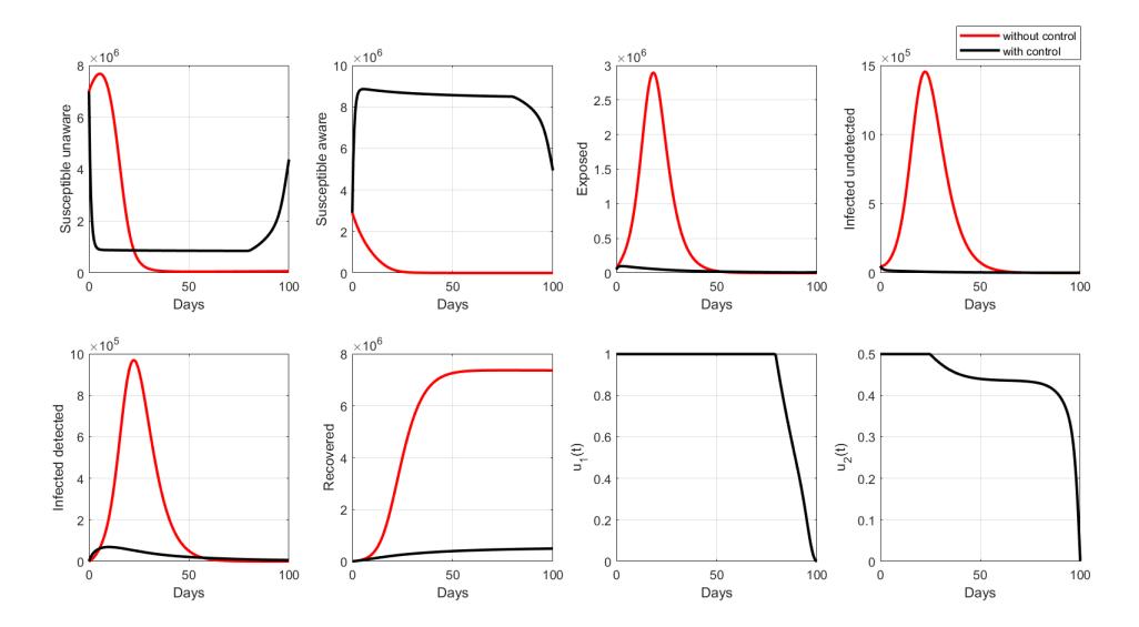
Figure 6: Trajectories of the state variables (6) and control variables for Scenario 1
Scenario 2: In some circumstances, the interventions cannot be carried out simultaneously among several available interventions. One reason is the limited intervention costs, or difficulty in implementation in the field. Therefore, Scenario 2 in this section describes the possibility of a media campaign intervention to increase social awareness being carried out as the sole intervention. The results can be seen in Figure 7.
Table 3: Numerical results of Scenario 1
| Cost Function with | Cost Function with | Number of Infec | Number of Humans | Total Cost of Inter |
|---|---|---|---|---|
| out Intervention | Intervention | tions Averted | Recovered | vention |
| 416.477 | 48.685 | 951.002 | 340.996 | 28.281 |
We can see that the dynamic of infected individuals when we rely solely on media campaign till succeeding in reducing the number of infected individuals. However, the result is not as good as in Scenario 1. It can be observed that the number of E, Iu, and Id still increases in the early period of simulation, due to two factors. First, we assume that media campaign interventions in our model are more about increasing social awareness of the dangers of COVID-19. In the equation (6), the role of social awareness reduces the chances of successful infection in the compartment of Sa. Therefore, the infection can still occur. The second reason is that when t = 0, the number of people in the exposed phase is already quite high. Without treatment and detection efforts by the government, people in the exposed stage will transform into infected individuals, who are ready to infect other people without any limitation. The numerical result due to the cost of intervention, number of infections averted and others due to Scenario 2 are presented in Table 4.
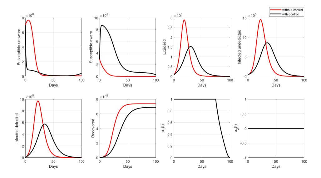
Figure 7: Trajectories of the state variables (6) and control variables for Scenario 2
Table 4: Numerical results of Scenario 2
| Cost Function with | Cost Function with | Number of Infec | Number of Humans | Total Cost Produced |
|---|---|---|---|---|
| out Intervention | Intervention | tions Averted | Recovered | by Intervention |
| 416.477 | 397.593 | 65.623 | 4.345.195 | 7.948 |
Scenario 3: In this last simulation, we perform a numerical simulation for Scenario 3, relying only on rapid test as a single intervention. The result can be seen in Figure 8. As already stated in our model construction, rapid test intervention is administered to detect the infected individuals and isolate them, so that they do not infect other susceptible individuals. Due to its purpose, we can see from Figure 8 that the number of undetected individuals decreases significantly, and is lower compared to Scenario 2. Consequently, the number of infected individuals is much higher than in Scenario 2. To achieve this result, the intensity of rapid test
intervention should be high almost at all times of the simulation, and start decreasing when it approaches the final stage of simulation. The cost of intervention is given in Table 5.
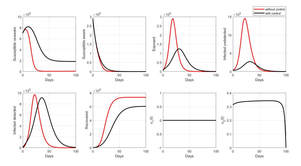
Figure 8: Trajectories of the state variables (6) and control variables for Scenario 3
Table 5: Numerical results of Scenario 3
| Cost Function with | Cost Function with | Number of Infec | Number of Humans | Total Cost Produced |
|---|---|---|---|---|
| out Intervention | Intervention | tions Averted | Recovered | by Intervention |
| 416.477 | 279.826 | 182.765 | 3.760.011 | 10.891 |
7.2. Cost-Effectiveness Analysis
Next, we perform a cost-effectiveness analysis of the optimal control strategy. We consider three methods to determine the best strategy, namely the Infection Averted Ratio (IAR), Average Cost-Effectiveness Ratio (ACER), and Incremental Cost-Effectiveness Ratio (ICER). The formula of the IAR is given by
\[IAR = \frac{\text{number of infection averted}}{\text{number of recovered}}.\]
From the description of the formula, IAR describes the level of success of the intervention based on the number of new infections avoided due to intervention, and number of those recovered due to the intervention; hence, the higher the value of IAR, the better the strategy. On the other hand, the formula of the ACER is given by
\[ACER = \frac{\text{total cost produced by intervention}}{\text{number of infection averted}},\] with the smallest IAR ratio is the best strategy. We can see that ACER describes an average of cost of intervention for each new infection that is successfully avoided due to the chosen intervention. Unlike the previous scenario, analysis of ICER is given by the following algorithm:
1) Rank the strategies by the number of infections averted from the smallest to the largest 2) For the first strategy,
\[ICER = \frac{\text{total cost produced by intervention}}{\text{total number of infections averted}}.\]
3) Next strategy,
\[ICER = \frac{\text{the difference between the total costs to n and n-1}}{\text{the difference between the number of infections averted to n and n-1}}.\]
- 4) Remove strategy with the largest ICER. Then, repeat step 2, 3 and 4 until two strategies remain
- 5) Choose the smallest ICER for the best strategy
The best strategy is the one with the smallest ICER ratio.
Table 6: IAR and ACER value of all Scenario
| Scenario | Number of Infec tions Averted | Number of Humans Recovered | Total Cost Produced by Intervention | IAR | ACER |
|---|---|---|---|---|---|
| 1 | 951.002 | 340.996 | 28.281 | 2, 79 | 0, 03 |
| 2 | 65.623 | 4.345.195 | 7.948 | 0, 02 | 0, 12 |
| 3 | 182.765 | 3.760.011 | 10.891 | 0, 05 | 0, 06 |
Using the results in Table 3,4 and 5, the value of IAR and ACER are given in Table 6. It can be seen that the best strategy for IAR is Strategy 1 when all interventions are administered, followed by Scenarios 3 and 2. This result means that to reduce the number of infected individuals significantly, all strategies should be implemented partially together. However, if a single intervention is to be administered, than choosing the rapid test to detect and isolate infected individuals is a more reasonable option than using media campaign to develop social awareness. A similar result is given for ACER value, where Scenario 3 is the best strategy to be implemented, followed by Scenario 3 and 2. These results tell us that although the cost of intervention for Scenario 1 is the highest compared to other scenarios, the average cost of each averted infected individual is the lowest. The reason is that each of these interventions has a different purpose. A high media campaign will reduce the number of new infected individuals due to social awareness, while rapid test is done to isolate infected individuals so that they cannot transmit COVID-19 to other people.
Table 7: ICER value for first elimination
| Number of Humans Total Cost Produced ICER by Intervention |
|---|
| 7.948 0, 12 |
| 10.891 0, 03 |
| 28.281 0, 02 |
Table 8: ICER value for second elimination
| Scenario | Number of Infec tions Averted | Number of Humans Recovered | Total Cost Produced by Intervention | ICER |
|---|---|---|---|---|
| 3 | 182.765 | 3.760.011 | 10.891 | 0, 06 |
| 1 | 951.002 | 340.996 | 28.281 | 0, 02 |
Based on the results of ICER as shown in Table 7 and 8, the best strategy is the combination of media campaign and rapid test to combat the spread of COVID-19. Hence, we can conclude that the implementation of media campaigns and rapid tests together is the best strategy to deal with the COVID-19 pandemic. However, when we have to choose one to be implemented as a single intervention, then rapid test is a more reasonable strategy.
8. CONCLUSIONS AND FUTURE WORK
This research introduces a mathematical model for COVID-19 transmission. The model considers several important factors such as the exposed phase of infection, detected and undetected cases, the intervention of media campaigns to increase social awareness, and a rapid test to detect and quarantine the infected individuals. Here are some summarized results
- 1) Mathematical analysis establishes a possible condition in the field, whether COVID-19 disappears (when the basic reproduction number is less than unity) or persists (when the basic reproduction number is larger than unity).
- 2) From the elasticity index, we found that the infection rate of COVID-19 is the most sensitive controllable parameter in our model.
- 3) Furthermore, we have identified that intervention by way of the rapid test is more sensitive in controlling the basic reproduction number, than media campaign.
- 4) From the optimal control simulation and cost-effectiveness analysis, it can be seen that conducting both interventions is significantly successful in avoiding a high level of the outbreak of disease, at a very low cost of intervention.
Although some important results are mentioned above, our model has several limitations that need to be addressed in future works.
- 1) It does not consider the vaccination strategy that has now been introduced in many countries. The question is, how big is the impact of the vaccine in controlling COVID-19?
- 2) Can we rely on the vaccination strategy alone to avoid a higher outbreak of COVID-19?
- 3) What percentage of the population must be vaccinated for herd immunity to be achieved?
- 4) Another limitation of our model is that we ignore a different type of virus that caused COVID-19. As mentioned by many other sources [20], several new strains of the virus are more deadly and spread with ease among humans.
ACKNOWLEDGEMENT
DA is funded by Universitas Indonesia with PUTI KI Q2 research grant scheme 2020, ID No : NKB-775/UN2.RST/HKP.05.00/2020.