

1. Introduction
Scalp electroencephalography (EEG) is a recording technique for the spontaneous electrical activity of the brain taken from the scalp, which is then correlated with to the underlying brain function [1]. Electroencephalography (EEG) is the most frequently used test for epilepsy patients [2], [3]. This technique can be used to diagnose epilepsy and determine the seizure disorder type and its place of origin [3].
Interictal Epileptiform Discharges (IEDs) has become the hallmark for epilepsy, with the ability to distinctly identify cortical hyperexcitability and hypersynchrony, which are present in the interictal state [1], [4]. One should be aware that in the evaluation of abnormalities in the EEG, many EEG transients that morphologically resemble epileptiform discharges and that need to be distinguished from diagnostically crucial epileptiform abnormalities to avoid overdiagnosis or misdiagnosis. These include benign epileptiform variants that must be recognized. Although morphologically similar, they are non-epileptogenic with no established relationship with the process responsible for generating epileptic seizures [1].
Misdiagnosis of epilepsy is relatively common. The main occurrence of misdiagnosis is the overinterpretation of normal EEG patterns as epileptiform [5]. There is enough evidence showing misinterpretation of benign EEG discharges, such as wicket spikes, which may result in misdiagnosis of epilepsy [6]. About 54% of wicket rhythms were incorrectly interpreted as an epileptiform activity. Whereas interobserver reliability is high in trained individuals, it is probably much less so in the real world, and EEG interpretation errors are not uncommon [4].
Some algorithms created from mathematical design have found, automated detection of interictal spikes with a positive predictive value of 92% and a sensitivity of 82% and different artifacts in the scalp EEG using Walsh- transformed EEG signals [7], [8]. Seizure prediction also has been designed by using an automatic Artificial Neural Network-Aided Diagnosis (ANNAD) system based on mathematical study for initial scalp
*Corresponding author
Received September \(29^{th}\), 2020, Revised December \(15^{th}\), 2020, Accepted for publication March \(30^{th}\), 2021. Copyright ©2021 Published by Indonesian Biomathematical Society, e-ISSN: 2549-2896, DOI:10.5614/cbms.2021.4.1.2
EEG screening to establish whether a given subject is epileptic or not [9]. The mathematical design of orthogonal operators based on the Walsh transform has also been made to detect the onset of epileptic seizures in intracranial EEG recordings [10]. Puspita et al. (2017a) propose two models to classify IEDS as spikes and sharp waves using the Bayesian approach based on the Walsh transformation profiles developed in Adjouadi et al. (2004, 2005) and Tito et al. (2007). The identification of the two IEDs using Backpropagation Neural Network based on the frequency and statistical features with different baselines on the upslope and downslope of IEDs is also presented by Puspita et al. (2017c). Similar to Puspita et al. (2017c), Puspita et al. (2017b) use frequency features with the same baseline for the upslope and downslope of the waves to identify spikes, sharp and wicket spikes using Backpropagation Neural Network. But so far, there are no mathematics formulas that were designed to differentiate interictal discharges and variants. The aim of our study is to differentiate wicket from IEDs using simple mathematics formulas for quantitative pattern recognition. This study uses the feature extraction simulation in Puspita et al. (2017b, 2017c) to measure the variables of the formula, namely amplitude, duration and angles.
This article is organized as follows. The methods for patient selection and data acquisition as well as the statistical analysis, are proposed in Section 2. Section 3 presents the results. The discussion is given in Section 4. Finally, Section 5 gives the conclusions.
2. MATERIAL AND METHODS
2.1. Patient Selection and Data Acquisition
We retrospectively analyzed EEG's Report of patients done in the EEG laboratory at Hasan Sadikin Hospital Bandung Indonesia, between July 2010 and June 2014 by using one Vyasis NicoletOne V32 EEG machine. All reports which contain IEDs in the form of spike and sharp waves and normal variant wicket spikes were retrieved and reanalyzed. Out of 1358 EEG records of adult patients, 604 showed IEDs and wicket spikes. Only EEGs of patients aged 30 years and above with temporal location of spikes and sharp waves, and wicket spikes without interfering artefacts on the particular waves, were included in this study.
IEDs should meet at least the following criteria [1], [16], [17]:
- 1) They should be paroxysmal.
- 2) They have to include an abrupt change in polarity occurring over several milliseconds which results in the sharp contour or "spikiness" of IED.
- 3) The duration of each transient should be less than 200 milliseconds. Spikes have a duration of less than 70 milliseconds, and sharp waves have a duration between 70 and 200 milliseconds.
- 4) The discharge should have a physiological field. IEDs are of negative polarity at the scalp, and the majority of IEDs are followed by a slow wave in the range of 2 to 4 Hz.
Wicket spikes are monophasic arciform discharges that appearing as single events or as brief runs at 6–11 Hz and recorded over the temporal head regions. Further they are characterized as unilateral or independently bilateral surface negative signals of 60–210 mV amplitude [6].
One hundred and forty-three EEGs were eligible for this study. However, only a few wicket spikes were found, thus all wicket spikes will be used in this study. We used 143 wicket spike data, 155 spike data, and 242 sharp data. Referential to average montage was used to choose the highest peak. The data were then converted to EEG Digital Format (EDF) files within the EEG machine itself, and then to American Standard Code for Infromation Intrechange (ASCII) files using Polyman Software. Amplitude (A), duration (T, ∆T1, and ∆T2) and angles (α and β) were measured from the wave triangles, as proposed in Puspita et al. (2017c), seen in Figure 1 and were taken as variables.
Two stages of analysis were performed, first to create the formula and second to see the goodness of the model based on the performance measures. Therefore, the collected data from each group were divided into training datasets (80%) and testing datasets (the remaining 20%).
2.2. Statistical Analysis
R software was used for all statistical analyses. Spearman correlation was used to measure the strength of the relationship between two variables. Further, Saphiro-Wilk normality test was performed to see the distribution of each variable in each group. Linear discriminant analysis was performed to create the formula for differentiating spike, sharp and wicket spike. Furthermore, we can compute the mean value of the
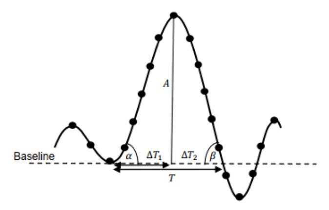
Figure 1: Illustration of variables measurement with a baseline.
discriminant function for each group in the training datasets, which is denoted by µi , for i = 1, 2, 3 represent spike, sharp, and wicket spike, respectively. This mean values are needed to calculate the cut-off scores. Cut-off score is the mean of the group centroid to classify the testing datasets into groups. The optimal cut-off score between groups 1 and 2 if the group sizes are equal is as follows:
\[CS_{opt} = \frac{N_1 Z_2 + N_2 Z_1}{N_1 + N_2},\tag{1}\] where N1, N2 are sizes of group 1 and 2, respectively, and Z1, Z2 are centroids of group 1 and 2, respectively [14]. In this case, the centroid is defined by µj , for a group j. Let f(X) be the linear discrimiant function defined as follows:
\[f(X) = c_0 + c_1 X_1 + c_2 X_2 + \dots + c_n X_n\] (2)
where X = (X1, X2, ..., Xn) is independent or predictor variable and ci , for i = 0, 1, 2..., n, is the discriminant coefficient for predictor variable, with n denotes the number of predictor variables [15]. If the discriminant function value, f(X), is bigger than cut-off score, CSopt, then the corresponding data is classified as group 1 and if it is less than cut-off score, then the corresponding data is classified as group 2 [15].
3. RESULTS
In this study, we require datasets with equal numbers of spike, sharp, and wicket spike waves. Thus, the spike and wicket spike data will be taken randomly until the number of spike and wicket spike data equal to sharp data. Figure 2 shows the correlation coefficient of all variables for each group using Spearman correlation. It can be seen that there are variables that give a high correlation coefficient value in one group, but not in the other group, such as the relationship between amplitude and α angle in the spike group. Therefore, all waves' variables will be used in this study.
The Saphiro-Wilks analysis showed a not normal distribution for all waves' variables because of the p − value < 0.05, as presented in Table 1. Thus, we transformed the value of all waves' variables using logtransform based on the skewness coefficient value, where a negative value means the distribution is negatively skewed and a positive value means the distribution is positively skewed. On the other hand, transformed data may also improve the classification accuracy. The Saphiro-Wilk normality test for transformed data is shown in Table 2. The variables that are still not normal do not significantly affect the resulting formula.
We divided the transformed data into 582 of training data to create the formula that can distinguish spike, sharp, and wicket spike waves, and 144 of testing data to validate the formula, randomly. Then, we applied the linear discriminant analysis method. To evaluate the performance of the resulting formula, accuracy was considered. We performed this procedure with ten repetitions to see the consistency of accuracy of the resulting formula. The accuracy for ten repetitions are shown in Table 3. The accuracy ranged between 91 and 97%.
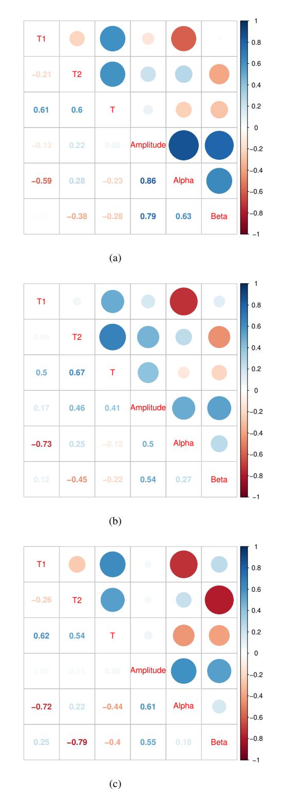
Figure 2: Spearman correlation of variable of (a) spike wave; (b) sharp wave; and (c) wicket spike wave.
Table 1: Saphiro-Wilk Normality Test and Skewness Coefficient.
| Type Wave | Variable | Skewness | p-value | Distribution |
|---|---|---|---|---|
| Spike | \(\Delta T_1\) | 0.046 | \(9.413 \times 10^{-4}\) | Not normal |
| • | \(\Delta T_2\) | 0.413 | \(7.973 \times 10^{-4}\) | Not normal |
| Duration \((T)\) | -0.345 | \(4.58 \times 10^{-5}\) | Not normal | |
| Amplitude \((A)\) | 2.043 | \(3.142 \times 10^{-16}\) | Not normal | |
| \(\alpha\) angle | -0.289 | \(9.234 \times 10^{-6}\) | Not normal | |
| \(\beta\) angle | -0.570 | \(3.966 \times 10^{-4}\) | Not normal | |
| Sharp | \(\Delta T_1\) | 0.614 | \(6.136 \times 10^{-9}\) | Not normal |
| \(\Delta T_2\) | 0.954 | \(2.663 \times 10^{-8}\) | Not normal | |
| Duration \((T)\) | 0.995 | \(2.17 \times 10^{-10}\) | Not normal | |
| Amplitude \((A)\) | 2.430 | \(< 2.2 \times 10^{-16}\) | Not normal | |
| \(\alpha\) angle | -0.352 | \(5.843 \times 10^{-5}\) | Not normal | |
| \(\beta\) angle | -0.475 | \(5.324 \times 10^{-3}\) | Not normal | |
| Wicket spike | \(\Delta T_1\) | 0.267 | \(1.905 \times 10^{-2}\) | Not normal |
| \(\Delta T_2\) | 0.542 | \(3.607 \times 10^{-5}\) | Not normal | |
| Duration \((T)\) | 0.788 | \(2.667 \times 10^{-9}\) | Not normal | |
| Amplitude \((A)\) | 1.584 | \(2.278 \times 10^{-13}\) | Not normal | |
| \(\alpha\) angle | -0.0170 | \(3.845 \times 10^{-2}\) | Not normal | |
| \(\beta\) angle | -0.304 | \(1.325 \times 10^{-2}\) | Not normal |
Table 2: Saphiro-Wilk Normality Test of Transformed Data.
| Type Wave | Variable | p-value | Distribution |
|---|---|---|---|
| Spike | \(\Delta T_1\) | \(9.553 \times 10^{-6}\) | Not normal |
| \(\Delta T_2\) | \(1.085 \times 10^{-5}\) | Not normal | |
| Duration \((T)\) | \(< 2.2 \times 10^{-16}\) | Not normal | |
| Amplitude \((A)\) | \(2.642 \times 10^{-5}\) | Not normal | |
| \(\alpha\) angle | \(6.301 \times 10^{-9}\) | Not normal | |
| \(\beta\) angle | \(4.665 \times 10^{-10}\) | Not normal | |
| Sharp | \(\Delta T_1\) | \(9.958 \times 10^{-10}\) | Not normal |
| \(\Delta T_2\) | 0.15 | Normal | |
| Duration \((T)\) | \(7.431 \times 10^{-7}\) | Not normal | |
| Amplitude \((A)\) | \(3.958 \times 10^{-5}\) | Not normal | |
| \(\alpha\) angle | \(9.612 \times 10^{-8}\) | Not normal | |
| \(\beta\) angle | \(3.315 \times 10^{-9}\) | Not normal | |
| Wicket spike | \(\Delta T_1\) | 0.010 | Not normal |
| \(\Delta T_2\) | 0.052 | Normal | |
| Duration \((T)\) | \(1.754 \times 10^{-7}\) | Not normal | |
| Amplitude \((A)\) | \(1.204 \times 10^{-8}\) | Not normal | |
| \(\alpha\) angle | \(2.224 \times 10^{-10}\) | Not normal | |
| \(\beta\) angle | \(2.346 \times 10^{-10}\) | Not normal |
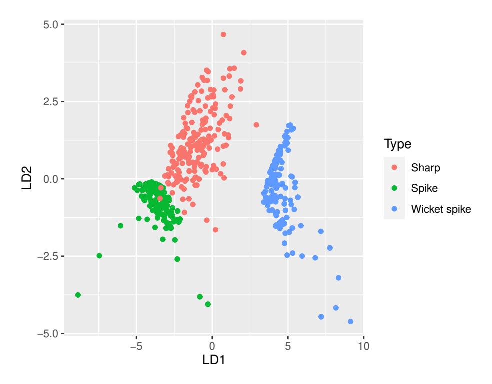
Figure 3: Distribution of training data.
Table 3: Accuracy.
| Repetition | Accuracy |
|---|---|
| 1 | 91.67% |
| 2 | 97.22% |
| 3 | 95.14% |
| 4 | 93.06% |
| 5 | 97.22% |
| 6 | 95.83% |
| 7 | 95.14% |
| 8 | 95.83% |
| 9 | 94.44% |
| 10 | 94.44% |
Table 4: Canonical Linear Discriminant Function Coefficients.
| Variable | LD 1 | LD 2 |
| ∆T1 | 13.031 | -12.062 |
| ∆T2 | 13.920 | -0.844 |
| T | 5.178 | 2.763 |
| Amplitude (A) | -23.607 | 20.588 |
| α angle | -8.787 | 11.439 |
| β angle | -7.891 | 3.982 |
| Proportion of trace | 0.940 | 0.060 |
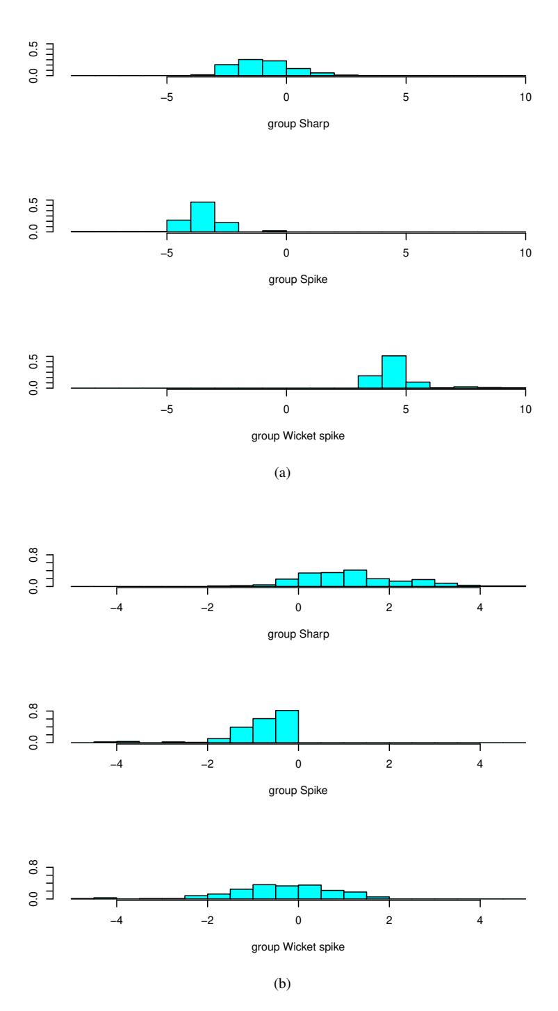
Figure 4: Histogram of (a) the first discriminant function's values (LD 1); (b) the second discriminant function's values (LD 2).
We choose the best formula based on the highest accuracy in Table 3. Therefore, the variable coefficient of linear discriminant function can be seen in Table 4. The trace proportion value represents the percentage separation achieved by each linear discriminant function. Thus, the first linear discriminant function (LD 1) can be used to achieve a good separation of the three groups. In addition, the histogram in Figure 4 shows that the wicket spike group is well separated from the IEDs group (spike and sharp) by the first linear discriminant function. Therefore, we obtain a formula to differentiate spike, sharp and wicket spike waves as follows
\[f(X^*) = 13.031\Delta T_1 + 13.920\Delta T_2 + 5.178T - 23.607A - 8.787\alpha - 7.891\beta, \tag{3}\]
where \(X^* = (\Delta T_1^*, \Delta T_2^*, T^*, A^*, \alpha^*, \beta^*)\) is a wave profile data. We also obtain the mean value of spike, sharp, and wicket spike based on the value of formula (3) to calculate the cut-off scores, with \(\mu_1 = -3.522\), \(\mu_2 = -1.008\), and \(\mu_3 = 4.530\). Thus, the following cut-off scores are obtained,
\[CS_1 = \frac{\mu_1 + \mu_2}{2} = -2.265\]
\(CS_2 = \frac{\mu_2 + \mu_3}{2} = 1.761.\)
where the three groups have the same number of data. The cut-off score to distinguish spike and sharp waves is \(CS_1\), where if \(f(X^*) \leq CS_1\) then \(X^*\) is classified as spike, otherwise as sharp. Meanwhile, \(CS_2\) is used as cut-off score to differentiate sharp from wicket spike, where \(f(X^*) \leq CS_2\) then \(X^*\) is classified as sharp, otherwise as wicket spike. Therefore, we have the classification rules determined by the two cut-off scores are as follows:
- if \(f(X^*) \leq CS_1\), then the wave with profile \(X^*\) will be considered as spike;
- if \(CS_1 < f(X^*) \le CS_2\) then it will be considered as sharp; and
- if \(f(X^*) > CS_2\) then it will be considered as wicket spike.
4. DISCUSSION
An EEG interpreter must have clear criteria for distinguishing relevant epileptiform discharges from sharply contoured background activity or benign variants. But wicket spikes still present a diagnostic challenge to nonepileptologists [1], [5]. The definition of spikes and sharp waves from the International Federation of Societies of clinical Neurophysiology is in fact, purely a morphological description of waveforms [16]. Differentiating normal variants from meaningful spikes and sharp waves can, at times, be challenging, applicable rules have been described. Unfortunately, they are only well known by EEG and epilepsy specialists, and in practices, most EEGs are read by general neurologists [5].
5. CONCLUSION
We have successfully constructed simple and applicable formula that can differentiate wicket spike from IEDs consisting of spikes and sharp waves with good accuracy. Linear discriminant analysis is applied to construct this formula using a wave variable consisting of amplitude, duration, and angles formed from the wave triangle based on a selected baseline. In this study, variable data transformation is needed to improve the classification accuracy of the resulting formula.
ACKNOWLEDGMENT
The authors gratefully acknowledge the cooperation of Mrs. Astini Salihima M.Sc. for the statistical analysis. Part of the work of the authors JWP, SWI and ES is funded by P3MI-ITB Research Grant.