

1. INTRODUCTION
Dengue fever has been recognized as a disease caused by the DENV virus. It is known that the Aedes aegypti mosquito is the main vector that transmits the virus from infected mosquitoes to humans. Currently, dengue fever has become an epidemic in most tropical and sub-tropical countries. Recent facts on dengue reported that outbreaks have also occurred in countries with no previous local transmission, such as in Oman in 2018-2019 [1]. With no currently-approved vaccine to treat dengue fever, the main strategy to prevent and control the spread of dengue fever is to control the mosquito population [2].
Various deterministic models for dengue fever transmission have been developed, following the simple SIR-SI model [3]. For deterministic models, the basic reproduction number (R0), which represents the expected number of secondary infections produced by a single typical infectious individual in a completely susceptible population, is the primary indicator for a region's endemicity [4]. We start with a deterministic model of SEIR-SEI type which will be the basis for the construction of the stochastic model.
The spread of dengue fever can be controlled by treating the human and the mosquito populations [5]. Mathematical models to control the spread of dengue by treating it in human populations have been developed. One model with human population controls using repellents has been studied in [6]. Also, Abidemi et al. in [7], developed a model involving eight mutually exclusive compartments by introducing personal protection, larvicide, and adulticide control strategies that illustrate the dynamics of dengue fever transmission.
Meanwhile, there are more ways to control the spread of dengue fever through the mosquito population. Various important factors of the mosquito population can be involved in controlling the mosquito population, such as the life cycle of mosquitoes [8], sterilizing male mosquitoes [9], releasing Wolbachia mosquitoes[10], and providing fogging [11]. Pliego et al. introduced a mathematical model of the Aedes aegypti mosquito's life cycle in water and air, which is also known as the two-stage life cycle [5]. The model reflecting changes in mosquito abundance was then modified with three seasonally adjusted control measures. Meanwhile, Wijaya et al., in their 2014 and 2016 research, explored a multi-age-class model for mosquito populations that were secondary classified into indoor-outdoor dynamics [12], [13].
*Corresponding author
As an endemic indicator, the basic reproduction number only gives the potential of endemic occurrence at the early infection period. With this indicator, the outbreak and possible disappearance of the disease cannot be described. In this respect, a stochastic approach will give more description of the intensity of the infection.
Here we consider a simple vector-host stochastic model where there is intervention in the vector population with fogging treatment and intervention in the host population by using an effective vector (mosquito) repellent. Our goal is to determine the efficacy of these intervention measures with respect to the rate of disease spread and the probability of disease extinction.
2. DETERMINISTIC MODEL
We start with a deterministic model of SEIR-SEI type which will be the basis for the construction of the stochastic model.
2.1. Model Development
Let \(S_h(t), E_h(t), I_h(t)\), and \(R_h(t)\) represent the number of susceptible, exposed (infected but not yet infectious), infectious, and recovered humans (hosts) after \(t \geq 0\) days, respectively. Similarly, let \(S_v(t), E_v(t)\), and \(I_v(t)\) denote the number of susceptible, exposed, and infectious mosquitoes (vectors) after \(t \geq 0\) days, respectively. The total human population will be denoted as \(N_h(t) = S_h(t) + E_h(t) + I_h(t) + R_h(t)\) and the total mosquito population will be denoted as \(N_v(t) = S_v(t) + E_v(t) + I_v(t)\). The formulation of the deterministic model is as follows:
\[\dot{S}_{h} = A_{h} - (1 - \tau)\beta_{h} \frac{S_{h}}{N_{h}} I_{v} - \mu_{h} S_{h}, \dot{E}_{h} = (1 - \tau)\beta_{h} \frac{S_{h}}{N_{h}} I_{v} - (\varphi_{h} + \mu_{h}) E_{h}, \dot{I}_{h} = \varphi_{h} E_{h} - (\gamma_{h} + \mu_{h}) I_{h}, \dot{R}_{h} = \gamma_{h} I_{h} - \mu_{h} R_{h}, \dot{S}_{v} = A_{v} - (1 - \tau)\beta_{v} S_{v} \frac{I_{h}}{N_{h}} - (\mu_{v} + \theta_{v}) S_{v}, \dot{E}_{v} = (1 - \tau)\beta_{v} S_{v} \frac{I_{h}}{N_{h}} - (\varphi_{v} + \mu_{v} + \theta_{v}) E_{v}, \dot{I}_{v} = \varphi_{v} E_{v} - (\mu_{v} + \theta_{v}) I_{v}.\] (1)
The parameters \(A_h>0\) and \(A_v>0\) represent recruitment rates for the host and vector populations, respectively, whereas the parameters \(\mu_h>0\) and \(\mu_v>0\) represent the natural death rates for the host and vector, respectively. The parameter \(\theta_v\geq 0\) denotes the fogging-related death rate of the vector population. We assume frequency-dependent disease transmission from vector to host and host to vector with transmission parameters \(\beta_h>0\) and \(\beta_v>0\), respectively. The parameter \(\tau\in[0,1]\) represents the proportion of the host population which is protected against vector contact with an effective repellent. The expressions \(1/\varphi_h\) and \(1/\varphi_v\) denote the duration of latency for infected hosts and vectors, respectively, where \(\varphi_h>0\) and \(\varphi_v>0\). Lastly, \(\gamma_h>0\) represents the recovery rate for infectious hosts. The total human and vector population dynamics are given by
\[\frac{dN_h}{dt} = A_h - \mu_h N_h, \frac{dN_v}{dt} = A_v - (\mu_v + \theta_v) N_v.\] (2)
For simplification, we assume that the human and vector populations are constant, and given by
\[N_h = \frac{A_h}{\mu_h},\] \[N_v = \frac{A_v}{\mu_v + \theta_v}.\] (3)
Thus the feasible region for the System (1) is
\[\Omega = \{ (S_h, E_h, I_h, R_h, S_v, E_v, I_v) | 0 \le S_v, E_v, I_v \le N_v, 0 \le S_h, E_h, I_h, R_h \le N_h S_v + E_v + I_v = N_v, S_h + E_h + I_h + R_h = N_h \}.\] (4)
Note that the domain \(\Omega\) is positively invariant under the System (1) since the vector fields on the boundary of \(\Omega\) do not point to the exterior.
2.2. The Basic Reproduction Number
The deterministic model (1) has a unique disease-free equilibrium (DFE) given by
\[DFE = (S_h, E_h, I_h, R_h, S_v, E_v, I_v) = (\bar{S}_h, 0, 0, 0, \bar{S}_v, 0, 0),\] (5)
where \(\bar{S}_h = A_h/\mu_h\) and \(\bar{S}_v = A_v/(\mu_v + \theta_v)\). The state variables representing infected hosts and vectors are \(E_h\), \(I_h\), \(E_v\), and \(I_v\). Linearizing the differential equations for these infected states about the unique DFE, we obtain the Jacobian matrix.
\[J = \begin{bmatrix} -(\mu_h + \varphi_h) & 0 & 0 & (1 - \tau)\beta_h \\ \varphi_h & -(\mu_h + \gamma_h) & 0 & 0 \\ 0 & (1 - \tau)\beta_v \frac{\bar{S}_v}{\bar{S}_h} & -(\mu_v + \varphi_v + \theta_v) & 0 \\ 0 & 0 & \varphi_v & -(\mu_v + \theta_v) \end{bmatrix}\](6)
The Jacobian can be expressed as J = F - V, where
\[F = \begin{bmatrix} 0 & 0 & 0 & (1-\tau)\beta_h \\ 0 & 0 & 0 & 0 \\ 0 & (1-\tau)\beta_v \frac{\bar{S}_v}{\bar{S}_h} & 0 & 0 \\ 0 & 0 & 0 & 0 \end{bmatrix},\] \[V = \begin{bmatrix} \varphi_h + \mu_h & 0 & 0 & 0 \\ -\varphi_h & \gamma_h + \mu_h & 0 & 0 \\ 0 & 0 & \varphi_v + \mu_v + \theta_v & 0 \\ 0 & 0 & -\varphi_v & \mu_v + \theta_v \end{bmatrix}\] \[(7)\]
The elements of matrix F correspond to the appearance of new infectious hosts or vectors and the elements of matrix V represent all other state transitions. The next generation matrix (NGM) is defined as
\[FV^{-1} = \begin{bmatrix} 0 & 0 & \frac{\varphi_v(1-\tau)\beta_h}{(\varphi_v + \mu_v + \theta_v)(\mu_v + \theta_v)} & \frac{(1-\tau)\beta_h}{\mu_v + \theta_v} \\ 0 & 0 & 0 & 0 \\ \frac{\varphi_h(1-\tau)\beta_v\bar{S}_v}{(\varphi_h + \mu_h)(\gamma_h + \mu_h)\bar{S}_h} & \frac{(1-\tau)\beta_v\bar{S}_v}{(\gamma_h + \mu_h)\bar{S}_h} & 0 & 0 \\ 0 & 0 & 0 & 0 \end{bmatrix}\](8)
The NGM spectral radius is defined as the basic reproduction number [23], [24]. That is,
\[\mathcal{R}_0 = \rho(FV^{-1}) = (1 - \tau)\sqrt{\frac{\varphi_v \beta_h \varphi_h \hat{\beta}_v}{(\varphi_v + \mu_v + \theta_v)(\mu_v + \theta_v)(\varphi_h + \mu_h)(\gamma_h + \mu_h)}},\tag{9}\]
where \(\hat{\beta}_v = \beta_v \bar{S}_v / \bar{S}_h\).
The basic reproduction number \(\mathcal{R}_0\) represents the expected number of secondary infections produced by a typical infectious individual in a completely susceptible population. For deterministic models, it is common that the basic reproduction number is a threshold. If \(\mathcal{R}_0 < 1\), the disease becomes extinct and if \(\mathcal{R}_0 > 1\), the disease will spread and become endemic within the population. From Equation (9), it can be seen that an increase in the transmission rates \(\beta_h\) and \(\beta_v\) will increase the value of \(\mathcal{R}_0\). Similarly, an increase in the fogging-related death rate \(\theta_v\) or the proportion of hosts using repellent \(\tau\), will decrease the value of \(\mathcal{R}_0\). The effects of the parameters on \(\mathcal{R}_0\) will be explored in more detail in the sensitivity analysis of \(\mathcal{R}_0\).
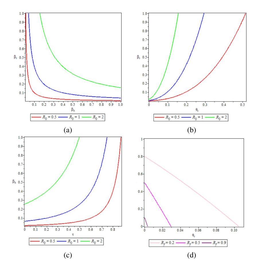
Figure 1: Level set of R0 and Rf .
2.3. Reduction Factor
Let us consider the basic reproduction number when there is no intervention by fogging or the use of repellent (θv = τ = 0). In this case, the basic reproduction number is given by
\[R_{00} = \sqrt{\frac{(\mu_v + \theta_v) \,\hat{\beta}_v \varphi_h \beta_h \varphi_v}{\mu_v^2 \left(\varphi_v + \mu_v\right) \left(\mu_h + \varphi_h\right) \left(\gamma_h + \mu_h\right)}}.\] (10)
Then after intervention, we have the reduction factor
\[\mathcal{R}_f = \sqrt{\frac{\left(-1+\tau\right)^2 \mu_v^2 \left(\varphi_v + \mu_v\right)}{\left(\mu_v + \theta_v\right)^2 \left(\varphi_v + \mu_v + \theta_v\right)}},\tag{11}\] so that R0 = RfR00.
In Figure 1, we see the sensitivity of the reduction factor Rf for variations in θv and τ , based on the data in Table 2.
3. STOCHASTIC MODEL
3.1. Continuous-Time Markov Chain Model
Let \(S_h(t), E_h(t), I_h(t)\), and \(R_h(t)\) denote discrete random variables which represent the number of susceptible, exposed (infected but not yet infectious), infectious, and recovered humans (hosts) after \(t \ge 0\) days, respectively. Similarly, let \(S_v(t)\), \(E_v(t)\), and \(I_v(t)\) denote discrete random variables representing the number of susceptible, exposed, and infectious mosquitoes (vectors) after \(t \ge 0\) days, respectively. The associated discrete-valued random vector is denoted as
\[X(t) = (S_h(t), E_h(t), I_h(t), R_h(t), S_v(t), E_v(t), I_v(t)).\] (12)
A continuous-time Markov chain (CTMC) model is defined in terms of the state transitions that occur for the stochastic process \(\{X(t)|t \in [0,\infty)\}\) during an infinitesimally-small time period \(\Delta t\). The state transitions and corresponding rates are summarized in Table 1. The expression \(r\Delta t + o(\Delta t)\) is a very small transition probability for the change \(\Delta X(t) = X(t + \Delta t) - X(t)\).
| Description | Chara | D-4 |
|---|---|---|
| Description | Change | Rate, r |
| Host recruitment | \(S_h \to S_h + 1\) | \(A_h\) |
| Death of \(S_h\) | \(S_h \to S_h - 1\) | \(\mu_h S_h\) |
| Host infection | \((S_h, E_h) \to (S_h - 1, E_h + 1)\) | \[(1-\tau)\beta_h S_h I_v/N_h\] |
| Death of \(E_h\) | \(E_h \to E_h - 1\) | \(\mu_h E_h\) |
| Latent to infectious (host) | \((E_h, I_h) \to (E_h - 1, I_h + 1)\) | \(\varphi_h E_h\) |
| Death of \(I_h\) | \(I_h \to I_h - 1\) | \(\mu_h I_h\) |
| Host recovery | \((I_h, R_h) \to (I_h - 1, R_h + 1)\) | \(\gamma_h I_h\) |
| Death of \(R_h\) | \(R_h \to R_h - 1\) | \(\mu_h R_h\) |
| Vector recruitment | \(S_v \to S_v + 1\) | \(A_v\) |
| Death of \(S_v\) | \(S_v \to S_v - 1\) | \((\mu_v + \theta_v)S_v\) |
| Vector infection | \((S_v, E_v) \to (S_v - 1, E_v + 1)\) | \((1-\tau)\beta_v S_v I_h/N_h\) |
| Death of \(E_v\) | \(E_v \to E_v - 1\) | \((\mu_v + \theta_v)E_v\) |
| Latent to infectious (vector) | \((E_v, I_v) \to (E_v - 1, I_v + 1)\) | \(\varphi_v E_v\) |
| Death of \(I_v\) | \(I_v \to I_v - 1\) | \((\mu_v + \theta_v)I_v\) |
Table 1: State transitions and rates describing the CTMC model.
3.2. Branching Process
A Galton-Watson multitype branching process is used to approximate the nonlinear CTMC dynamics near the DFE. The only sources of infection for our model are the states \(E_h, I_h, E_v\), and \(I_v\). Therefore, the branching process estimates are applied only to these states and the numbers of susceptible humans and mosquitoes are assumed to be close to disease-free equilibrium., \(\bar{S}_h = A_h/\mu_h\) and \(\bar{S}_v = A_v/(\mu_v + \theta_v)\).
Susceptible hosts can become exposed through direct contact with an infectious vector. Similarly, susceptible vectors can become exposed by direct contact (i.e. biting) with an infectious host. In what follows, we use the term 'offspring' to describe susceptible hosts or vectors which become exposed by direct contact with an infectious vector or host, respectively. The term 'offspring' will also be used for exposed hosts or vectors which progress to a state of infectiousness. It is assumed that the number of offspring produced by a single human or an exposed / infectious mosquito does not depend on the number of offspring produced by humans or other exposed / infectious mosquitoes. Offspring probability generating functions (pgfs) is defined for the "birth" and "death" of an exposed or infected individual. The probability of disease extinction was calculated using pgf [15], [17], [19], [20], [21], [22].
In general, for \(x_i(0) = 1\) and \(x_i(0) = 0\) for \(i \neq i\), the offspring probability generating function (pgf) for individuals of type i is the function \(f_i:[0,1]^n\to[0,1]^n\) is defined by
\[f_i(x_1, \dots, x_n) = \sum_{k_1=1}^{\infty} \dots \sum_{k_n=1}^{\infty} P_i(k_1, \dots, k_n) x_1^{k_1} \dots x_n^{k_n},\] (13)
where \(P_i(k_1,\ldots,k_n)\) denotes the probability that one type i individual gives 'birth' to \(k_j\) individuals of type j. For the branching process approximation, we consider exposed hosts as type 1 individuals \((x_1)\), infectious hosts as type 2 individuals \((x_2)\), exposed vectors as type 3 individuals \((x_3)\), and infectious vectors as type 4 individuals \((x_4)\).
The offspring pgf for \(E_h\), given that \(E_h(0) = 1\), \(I_h(0) = 0\), \(E_v(0) = 0\), and \(I_v(0) = 0\) is
\[f_1(x_1, x_2, x_3, x_4) = \frac{\varphi_h x_2 + \mu_h}{\varphi_h + \mu_h}.\] (14)
The term \(\varphi_h/(\varphi_h + \mu_h)\) is the probability that an exposed host becomes infectious, and \(\mu_h/(\varphi_h + \mu_h)\) is the probability of natural death for an exposed host.
The offspring pgf for \(I_h\), given that \(E_h(0) = 0\), \(I_h(0) = 1\), \(E_v(0) = 0\), and \(I_v(0) = 0\) is
\[f_2(x_1, x_2, x_3, x_4) = \frac{(1 - \tau)\hat{\beta}_v x_2 x_3 + \mu_h + \gamma_h}{(1 - \tau)\hat{\beta}_v + \mu_h + \gamma_h}.\] (15)
The term \((1-\tau)\hat{\beta_v}/((1-\tau)\hat{\beta_v}+\mu_h+\gamma_h)\) is the probability that a susceptible vector becomes exposed from contact with an infectious host resulting in one infectious host and one exposed vector. The term \((\mu_h + \gamma_h)/((1-\tau)\beta_v + \mu_h + \gamma_h)\) is the probability that an infectious host dies or recovers.
The offspring pgf for \(E_v\), given that \(E_h(0) = 0\), \(I_h(0) = 0\), \(E_v(0) = 1\), and \(I_v(0) = 0\) is
\[f_3(x_1, x_2, x_3, x_4) = \frac{\varphi_v x_4 + \mu_v + \theta_v}{\varphi_v + \mu_v + \theta_v}.\] (16)
The term \(\varphi_v/(\varphi_v+\mu_v+\theta_v)\) is the probability that an exposed vector becomes infectious, and the term \((\mu_v+\theta_v)/(\varphi_v+\mu_v+\theta_v)\) is the probability that an exposed vector dies naturally or due to fogging. The offspring pgf for \(I_v\), given that \(E_h(0) = 0\), \(I_h(0) = 0\), \(E_v(0) = 0\), and \(I_v(0) = 1\) is
\[f_4(x_1, x_2, x_3, x_4) = \frac{(1 - \tau)\beta_h x_1 x_4 + \mu_v + \theta_v}{(1 - \tau)\beta_h + \mu_v + \theta_v}.\] (17)
The term \((1-\tau)\beta_h/((1-\tau)\beta_h+\mu_v+\theta_v)\) is the probability that a susceptible host becomes exposed from contact with an infectious vector resulting in one exposed host and one infectious vector. The term \((\mu_v + \theta_v)/((1-\tau)\beta_h + \mu_v + \theta_v)\) is the probability that an infectious vector dies naturally or due to fogging.
The offspring pgfs always have at least one fixed point in \([0,1]^4\) given by (1,1,1,1). If the offspring pgfs are nonsingular, then there exists a unique fixed point in \((0,1)^4\) [17], [19], [20], [22]. A function \(f_i\) is called singular if it is a linear function of \(x_j\), \(j=1,\ldots,4\) such that \(f_i(0,0,0,0)=0\). The expectation matrix \(M=[m_{ij}]\) for the offspring pgfs is a nonnegative \(4\times 4\) matrix, whose entries are defined as
\[m_{ij} = \frac{\partial f_j}{\partial x_i},\tag{18}\] where the partial derivatives are evaluated at \((x_1, x_2, x_3, x_4) = (1, 1, 1, 1)\). The entry \(m_{ij}\) denotes the expected number of type i offspring produced by one individual of type j. The expectation matrix for the offspring pgfs is
\[M = \begin{bmatrix} 0 & 0 & 0 & \frac{(1-\tau)\beta_h}{(1-\tau)\beta_h + \mu_v + \theta_v} \\ \frac{\varphi_h}{\varphi_h + \mu_h} & \frac{(1-\tau)\hat{\beta}_v}{(1-\tau)\hat{\beta}_v + \mu_h + \gamma_h} & 0 & 0 \\ 0 & \frac{(1-\tau)\hat{\beta}_v}{(1-\tau)\hat{\beta}_v + \mu_h + \gamma_h} & 0 & 0 \\ 0 & \frac{\varphi_v}{\varphi_v + \mu_v + \theta_v} & \frac{(1-\tau)\beta_h}{(1-\tau)\beta_h + \mu_v + \theta_v} \end{bmatrix}\](19)
Since the offspring pgfs \(f_i\) are nonsingular and the expectation matrix M is irreducible, there are at most two fixed points in \([0,1]^4\) [22]. If the process is subcritical or critical \((\rho(M) < 1 \text{ or } \rho(M) = 1)\), then (1,1,1,1) is the only fixed point, and if the process is supercritical \((\rho(M)>1)\), then there exists a unique
second fixed point \((q_1, q_2, q_3, q_4) \in (0, 1)^4\) of the offspring pgfs [17], [19], [20], [22]. This fixed point is used to calculate the probability of disease extinction [17], [19], [20], [22]. In particular, the probability of disease extinction is given by
\[P_0 = \begin{cases} 1 & \text{if } \rho(M) \le 1, \\ q_1^{E_h(0)} q_2^{I_h(0)} q_3^{E_v(0)} q_4^{I_v(0)} & \text{if } \rho(M) > 1. \end{cases}\] (20)
The terms \(q_1, q_2, q_3\), and \(q_4\) are the probability of disease extinction in the exposed host population, infectious host, exposed vector, and infectious vector, respectively. If \(\rho(M) > 1\), then the probability of a "major outbreak" can be defined as
\[1 - P_0 = 1 - q_1^{E_h(0)} q_2^{I_h(0)} q_3^{E_v(0)} q_4^{I_v(0)}.\] (21)
In this context, a "major outbreak" is considered anything other than disease extinction, opposed to the number of infectious individuals in the host or vector populations reaching some critical level.
The computation of the spectral radius M cannot be shown explicitly. However, the Threshold Theorem in [16] gives the following relationship between \(\rho(M)\) and \(R_0\):
\[R_0 < 1 \ (=1, > 1) \iff \rho(M) < 1 \ (=1, > 1).\] (22)
The hypotheses of the Threshold Theorem are satisfied since the expectation matrix M is irreducible, the matrix F in (6) is non-negative, and the matrix V in (6) is a nonsingular M-matrix.
The fixed point of the offspring pgfs can be calculated explicitly in terms of the model parameters:
\[q_1 = \frac{\varphi_h}{\varphi_h + \mu_h} q_2 + \frac{\mu_h}{\varphi_h + \mu_h}, \tag{23}\]
\[q_{2} = \frac{(1-\tau)\hat{\beta}_{v}\varphi_{v}}{(1-\tau)\hat{\beta}_{v}\varphi_{v} + (\varphi_{v} + \mu_{v} + \theta_{v})(\gamma_{h} + \mu_{h})} \frac{1}{R_{0}^{2}} + \frac{(\varphi_{v} + \mu_{v} + \theta_{v})(\gamma_{h} + \mu_{h})}{(1-\tau)\hat{\beta}_{v}\varphi_{v} + (\varphi_{v} + \mu_{v} + \theta_{v})(\gamma_{h} + \mu_{h})}, (24)\] \[q_{3} = \frac{\varphi_{v}}{\varphi_{v} + \mu_{v} + \theta_{v}} q_{4} + \frac{\mu_{v} + \theta_{v}}{\varphi_{v} + \mu_{v} + \theta_{v}}, \qquad (25)\] \[q_{4} = \frac{(1-\tau)\beta_{h}\varphi_{h}}{(1-\tau)\beta_{h}\varphi_{h} + (\mu_{v} + \theta_{v})(\varphi_{h} + \mu_{h})} \frac{1}{R_{0}^{2}} + \frac{(\mu_{v} + \theta_{v})(\varphi_{h} + \mu_{h})}{(1-\tau)\beta_{h}\varphi_{h} + (\mu_{v} + \theta_{v})(\varphi_{h} + \mu_{h})}. \qquad (26)\]
\[q_3 = \frac{\varphi_v}{\varphi_v + \mu_v + \theta_v} q_4 + \frac{\mu_v + \theta_v}{\varphi_v + \mu_v + \theta_v},\tag{25}\]
\[q_4 = \frac{(1-\tau)\beta_h \varphi_h}{(1-\tau)\beta_h \varphi_h + (\mu_v + \theta_v)(\varphi_h + \mu_h)} \frac{1}{R_0^2} + \frac{(\mu_v + \theta_v)(\varphi_h + \mu_h)}{(1-\tau)\beta_h \varphi_h + (\mu_v + \theta_v)(\varphi_h + \mu_h)}.\] (26)
The expressions for \(q_1\) and \(q_3\) follow directly from the definitions of the offspring pgfs \(f_1\) and \(f_3\). The expression for \(q_2\) (\(q_4\)) is the sum of two probabilities: (1) probability of successful transmission from one infectious human (mosquito) to a susceptible mosquito (human) times the probability of no secondary human infection (mosquito) \(1/R_0^2\) plus (2) possible transmission failure (death of humans or mosquitoes). Note that the expression \(R_0^2\) is a type of reproduction number to control for human or mosquito populations [?], [?].
In Section 4, we compare the results of the deterministic and stochastic models. Additionally, we compute the extinction probabilities \(q_1, \ldots, q_4\) using parameter values related to dengue transmission among humans and mosquitoes and show that the expression obtained for the probability of disease extinction from the branching process approximation agrees well with numerical simulations of the CTMC model. The effects of fogging and use of an effective mosquito repellent on \(R_0\) and \(P_0\) are explored numerically.
4. Numerical Simulations
We present numerical simulation resulting from the analysis in the previous sections.
4.1. Probability of Disease Extinction
The parameter values used for numerical simulations of the deterministic and stochastic models are given in Table 2. We assume baseline values of \(\theta_v = 0.1\) and \(\tau = 0.1\) for the fogging-related death rate and proportion of hosts protected with an effective repellent. These parameter values are variable and we explore the effects of varying \(\theta_v\) and \(\tau\) on the basic reproduction number and probability of disease extinction.
Using the parameter values in Table 2, the basic reproduction number is \(R_0 \approx 2.19\). Solutions of the deterministic model exhibit an initial outbreak in both the host and vector populations before stabilizing at an endemic level near disease extinction (i.e. \(E_h(t), I_h(t), E_v(t)\), and \(I_v(t) \approx 0\)). The ODE solution and one sample path of the CTMC model are plotted in Figure 2.
Table 2: Model parameters related to dengue transmission. The basic reproduction number for these parameters is \(R_0 \approx 2.19\).
| Description | Parameter | Value | Source |
|---|---|---|---|
| Host recruitment rate | \(A_h\) | \(1000 \cdot \mu_h\) | [6] |
| Host death rate | \(\mu_h\) | \(\frac{1}{70 \times 365}\) | [6] |
| Host infection rate | \(\beta_h\) | 0.375 | [3] |
| Host latentcy period | \(1/\varphi_h\) | 7 | Assumed |
| Host recovery rate | \(\gamma_h\) | 1/14 | [6] |
| Vector rectuirment rate | \(A_v\) | \[500 \cdot (\mu_v + \theta_v)\] | [6] |
| Vector natural death rate | \(\mu_v\) | \(\frac{1}{30}\) | [6] |
| Fogging-related death rate | \(\theta_v\) | 0.1 | Assumed |
| Vector infection rate | \(\beta_v\) | 0.5 | [3] |
| Vector latency period | \(1/\varphi_v\) | 5 | Assumed |
| Proportion of hosts using repellent | \(\tau\) | 0.1 | Assumed |
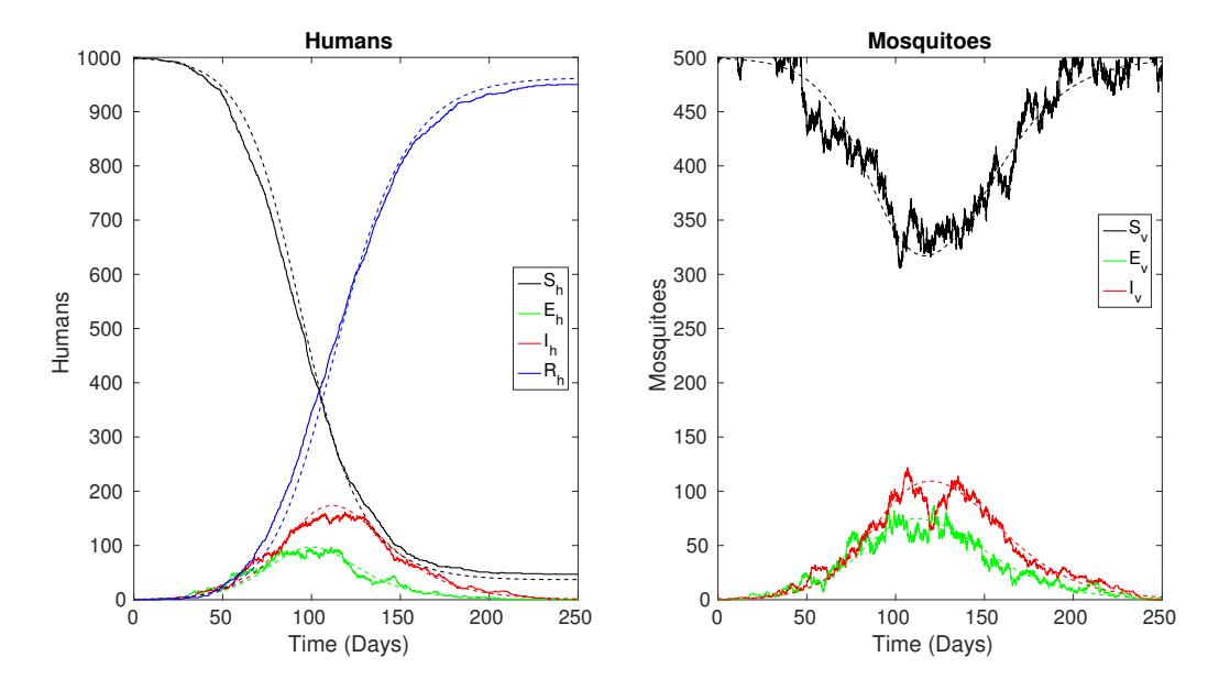
Figure 2: Comparison of one sample path of the CTMC model (solid line) and the ODE solution (dashed line). Parameter values are as in Table 2 with initial conditions \(S_h(0) = 999\), \(E_h(0) = 0\), \(I_h(0) = 1\), \(R_h(0) = 0\), \(S_v(0) = 499\), \(E_v(0) = 0\), and \(I_v(0) = 1\). The probability of disease extinction is \(P_0 = 0.2092\).
The probability of disease extinction is calculated for several sets of initial conditions using the expression in equation (21) obtained from the branching process approximation. This expression is compared to a numerical approximation obtained from the proportion of 10,000 sample paths of the CTMC model which exhibit disease extinction (i.e. \(E_h(t) = I_h(t) = E_v(t) = I_v(t) = 0\)) prior to time t = 150 which is approximately the time of peak infection for the ODE model. The results are summarized in Table 3.
The expressions for \(q_1, q_2, q_3\), and \(q_4\) in (23)-(26) represent the probability of disease extinction in the states \(E_h, I_h, E_v\), and \(I_v\), respectively. In Figure 3, the sensitivity of each of these quantities is shown to the fogging-related death rate, \(\theta_v\).
Table 3: Probability of disease extinction P0 and a numerical approximation (Approx.) based on 10,000 sample paths of the CTMC model with parameter values as in Table 2 and initial conditions Sh(0) = 1000, Eh(0), Ih(0), Rh(0) = 0, Sv(0) = 500, Ev(0), and Iv(0). The value of P0 was obtained from the expression in (21).
| Eh(0) | Ih(0) | Ev(0) | Iv(0) | P0 | Approx. |
|---|---|---|---|---|---|
| 1 | 0 | 0 | 0 | 0.4831 | 0.4831 |
| 0 | 1 | 0 | 0 | 0.4829 | 0.4834 |
| 0 | 0 | 1 | 0 | 0.6599 | 0.6564 |
| 0 | 0 | 0 | 1 | 0.4332 | 0.4398 |
| 1 | 0 | 1 | 0 | 0.3188 | 0.3204 |
| 0 | 1 | 0 | 1 | 0.2092 | 0.2092 |
| 1 | 1 | 0 | 0 | 0.2333 | 0.2350 |
| 0 | 0 | 1 | 1 | 0.2859 | 0.2809 |
| 1 | 1 | 1 | 1 | 0.0669 | 0.0653 |
| 2 | 0 | 0 | 0 | 0.2334 | 0.2374 |
| 0 | 2 | 0 | 0 | 0.2332 | 0.2336 |
| 0 | 0 | 2 | 0 | 0.4355 | 0.4366 |
| 0 | 0 | 0 | 2 | 0.1877 | 0.1875 |
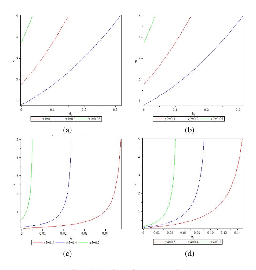
Figure 3: Level set of q1, q2, q3, and q4.
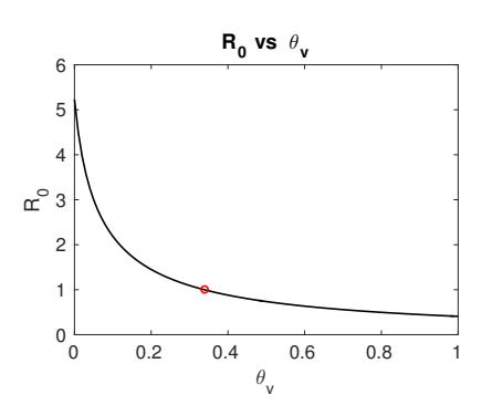
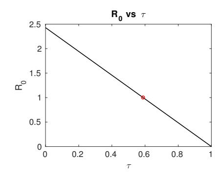
Figure 4: Plots of the basic reproduction number illustrating the effects of fogging and the use of effective repellent. Parameter values are as in Table 2 with the exception of \(\theta_v\) and \(\tau\) which vary over the domain \(0 \le \theta_v \le 1\) and \(0 \le \tau \le 1\), respectively. The red circle indicates the point at which \(\mathcal{R}_0 = 1\).
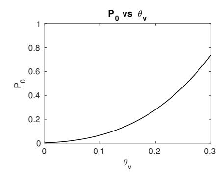
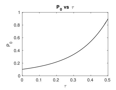
Figure 5: Plots of the probability of disease extinction \(P_0\) illustrating the effects of fogging and the use of an effective repellent. Parameter values are as in Table 2 with the exception of \(\theta_v\) and \(\tau\) which vary over the domain \(0 \le \theta_v \le 0.3\) and \(0 \le \tau \le 0.5\), respectively. The initial conditions used to calculated \(P_0\) are \(E_h(0) = 1\), \(I_h(0) = 1\), \(E_v(0) = 1\), and \(I_v(0) = 1\).
4.2. Control Efforts
In this section, we explore the utility of fogging and mosquito repellent. To explore the effects of fogging, we consider the basic reproduction number and probability of disease extinction as functions of the fogging-related death rate of vectors, \(R_0 = R_0(\theta_v)\) and \(P_0 = P_0(\theta_v)\), and allow \(\theta_v\) to vary over a domain of biologically-feasible values. Similarly, to explore the effects of mosquito repellent, we consider \(R_0\) and \(P_0\) as functions of \(\tau \in [0,1]\). We are primarily interested in the values of \(P_0\) for \(P_0 > 1\). Therefore, we only consider values of \(\theta_v\) and \(\tau\) for which \(P_0 > 1\) in our exploration of \(P_0\). In the subcritical (critical) case \(P_0 < 1\) (\(P_0 = 1\)), the probability of disease extinction is given by \(P_0 = 1\).
The effects of fogging and mosquito repellent can be seen in Figures 4 and 5. Recall that \(P_0\) is dependent on the initial number of exposed/infectious hosts and vectors. To gain a better understanding of the ways in which \(\theta_v\) and \(\tau\) affect the probability of disease extinction, we plot several of the level sets for the extinction probabilities \(q_1, \ldots, q_4\).
Control efforts may not be implemented until the number of infectious hosts reaches a critical level. It is of interest to determine the expected time at which the number of infectious individuals reaches this critical level. In Figure 6, we plot the approximate probability distribution for the time at which the number of infectious hosts reaches a threshold level of \(I_h(t) = 10\) prior to a maximum time of \(t_{\rm max} = 250\). Parameter values are as in Table 2 with initial conditions \(E_h(0) = 1\), \(I_h(0) = 1\), \(E_v(0) = 1\), and \(I_v(0) = 1\). The mean time at which the threshold is reached is \(\bar{t} = 51\) days. Calculations are based on 10,000 sample paths of the CTMC model. Note that approximately 6.5% of the sample paths exhibit disease extinction prior to reaching the treshold level resulting in the spike at tmax = 250 days. This is consistent with our expression for P0 given the same set of initial conditions (see Table 3).
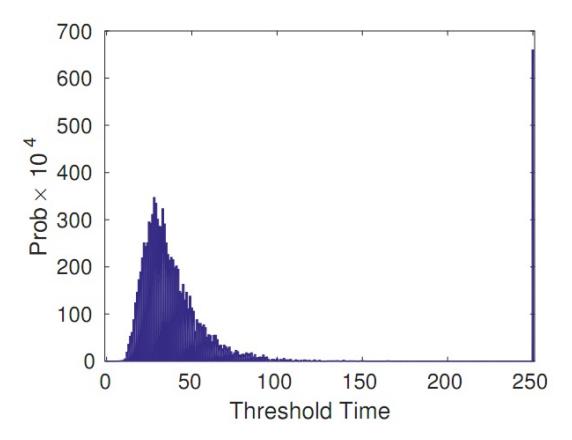
Figure 6: Approximate probability distribution for the time at which the number of infectious hosts reaches a threshold level of Ih(t) = 10 prior to a maximum time of tmax = 250. Parameter values are as in Table 2 with initial conditions Eh(0) = 1, Ih(0) = 1, Ev(0) = 1, and Iv(0) = 1. The mean time at which the threshold is reached is t¯ = 51 days. Calculations are based on 10,000 sample paths of the CTMC model.
4.3. Sensitivity Analysis
We calculate the sensitivity indices of the basic reproduction number, R0, and the probability of disease extinction P0, to the model parameters. How much influence each parameter is for disease transmission and outbreak / extinction is determined by these two indices.
To calculate the sensitivity indices, we use the normalized forward sensitivity index as defined in [18]. Specifically, the normalized variable forward sensitivity index, u, which depends on the parameter, p, is defined as
\[\Upsilon_p^u = \frac{\partial u}{\partial p} \times \frac{p}{u}.\tag{27}\]
Since we have a explicit expressions for R0 and P0 in 9 and 21, Two sensitivity indices R0 and P0 can be calculated for each parameter of the model in the Table 2.
4.4. Sensitivity Indices of R0
The sensitivity index of R0 with respect to τ is
\[\Upsilon_{\tau}^{\mathcal{R}_0} = -\frac{\tau}{1-\tau}.\tag{28}\]
The sensitivity index of R0 with respect to Ah is
\[\Upsilon_{A_h}^{\mathcal{R}_0} = -\frac{1}{2}.\tag{29}\]
The sensitivity index of R0 with respect to βh is
\[\Upsilon_{\beta_h}^{\mathcal{R}_0} = \frac{1}{2}.\tag{30}\]
The sensitivity index of R0 with respect to γh is
\[\Upsilon_{\gamma_h}^{\mathcal{R}_0} = -\frac{1}{2} \frac{\gamma_h}{\gamma_h + \mu_h}.\tag{31}\]
The sensitivity index of R0 with respect to Ah is
\[\Upsilon_{A_v}^{\mathcal{R}_0} = \frac{1}{2}.\tag{32}\]
\[\Upsilon_{\beta_v}^{\mathcal{R}_0} = \frac{1}{2}.\tag{33}\]
Table 4: Based on the basic parameter values given in Table 2, the indices of sensitivity of R0 to the parameters for the dengue 1 model is evaluated. The parameters are in order of the most sensitive. θv, the mosquito mortality rate related to fogging is the most sensitive parameter, and ϕh, the human rate of progression from the latent state is the least sensitive parameter.
| Parameter, p | R0 Sensitivity Index, Υ p |
|---|---|
| θv | −0.90 |
| Ah | −0.50 |
| µh | +0.50 |
| βh | +0.50 |
| Av | +0.50 |
| βv | 0.50 |
| γh | −0.50 |
| µv | −0.30 |
| ϕv | +0.20 |
| τ | −0.11 |
| ϕh | +0.00014 |
5. CONCLUSION
A continuous-time Markov chain model for the transmission of dengue fever with mosquito fogging and use of repellent was presented. Two control parameters are used in the model in the form of mosquito repellent for reducing the contacts between mosquitoes and humans, and in the form of fumigation (fogging) for reducing the mosquito population. In a multitype branching process approximation, the offspring probability generating functions for the infected states are constructed and the existence of a nontrivial fixed point which is related to the basic reproduction number is found. An expression for the probability of disease extinction is obtained and numerical simulations are performed including sensitivity analysis of the basic reproduction number. The results are expected to give a more comprehensive insight of dengue transmission.
ACKNOWLEDGEMENT
The author 2 acknowledges the support from the Indonesian RistekDikti HKLN grant 2018-2019.