

1. INTRODUCTION
Coronaviruses (CoVs) are large enveloped viruses with a single-stranded, unsegmented RNA genome that is positive in sense. It has the largest genome of any RNA. Because CoVs are RNA viruses, they can easily evolve through homologous and non-homologous mutation and recombination, allowing them to spread to a wider range of hosts [1]. COVID-19 was first reported in December 2019 in Wuhan, China, and was declared a pandemic by WHO on March 11, 2020, infecting around 170 million confirmed cases and resulting in over 3 million deaths [2],[3]. Thus, COVID-19 became a disease that emerged with a rapid increase in cases and deaths since the first identification [4]. COVID-19 spreads from person to person via direct contact with sneezing or coughing, or through contact with an infected person's secretions. Therefore, the mechanism of its spread is the same as that of a common cold virus or another influenza [5],[6]. COVID-19 pandemic is a global public health emergency with potentially catastrophic consequences. This pandemic has impacted the burden in tropical and subtropical regions of the world where dengue fever, caused by the dengue virus (DENV), is already prevalent. Concerns have been raised about the similar clinical manifestations of COVID-19 and dengue fever, particularly in dengue-endemic countries [7]. Coexistence of COVID-19 with other illnesses is not uncommon during the COVID-19 pandemic, and misdiagnosis is possible. These problems are particularly prevalent in tropical regions where other infectious illnesses, such as dengue fever, exhibit symptoms comparable to COVID-19[8][9]. In tropical countries, dengue is diagnosed by identifying distinctive symptoms such as fever and test abnormalities such as thrombocytopenia and capillary leakage[10]. Serological assays are being utilized to confirm dengue virus infection at the moment. Nonetheless, the resemblance in some symptoms between dengue and COVID-19, as well as the possibility of cross-reactions in serological testing, might lead to difficulties in diagnosis and is an essential topic to address [11].
Dengue is a common infection in the tropic and subtropic areas that is caused by the dengue virus (DENV) that transmitted by bite mosquitoes of Aedes Aegypty and Aedes albopictus. It is estimated that 400 million
*Corresponding Author
Received November 20th, 2021, Revised December 10th, 2021, Accepted for publication December 24th, 2021. Copyright ©2021 Published by Indonesian Biomathematical Society, e-ISSN: 2549-2896, DOI:10.5614/cbms.2021.4.2.5
dengue infections occur each year, caused by four antigenically related but distinct viruses, DENV-1, DENV-2, DENV-3, and DENV-4 [12]. Primary infection with one of the serotypes is usually not dangerous, even if some people develop asymptoms [15]. Because there is no immunity, secondary infection by other serotypes can be more severe and lead to life-threatening conditions such as Dengue Haemorrhagic Fever or Dengue Shock Syndrome (DSS) [14]. In recent years, mathematical modeling has become an important tool for understanding the epidemiology and dynamics of infectious diseases. Multi-strain dengue dynamics have been modeled at the population level using extended (susceptible-infected-recovered) SIR-type models that include immunological aspects of the disease such as temporary cross-immunity and ADE phenomenology [15],[16]. Pongsumpun et al. [17] have studied a mathematical model of Dengue Hemorrhagic Fever (DHF) transmission in a two-age structure in the human population, namely Juveniles class and adults class. Nuraini et al. has studied dengue transmission models with two strains involving the role of immunity [18]. In addition, they have also built a within-host model involving cells, viruses, and immunity [19].
Several investigations have found false-positive dengue serology findings in individuals with COVID-19. Coinfection of COVID-19 and dengue have been found and confirmed in several countries, including Argentina with 13 cases, Singapore with 2 cases and Indonesia with 1 case [20],[21],[22]. To simply explain coinfection transmission and when it can occur, mathematical models with various assumptions have been explored and evaluated, with a focus on evaluating the components that allow widespread transmission and controlling for pathogen transmission [24]. We developed the Susceptible-Invected-Recovered model by Kermack and McKendrick in 1927 [25]. One of the tools that facilitate the understanding of the spread of infectious diseases is mathematical modeling. Several mathematical approaches to study the dengue transmission, the COVID transmission and coinfection of COVID-19 and dengue dynamics which Nuraini et al.[26] proposed a mathematical model of dengue internal transmission process, Samui et al.[27] proposed a mathematical model for COVID-19 transmission dynamics with a case study of India, furthermore Masyeni et al.[22] serological cross-reaction and co-infection of COVID-19 and dengue in Asia: experience from Indonesia. Yang et al. [23] developed a mathematical model encompassing two subpopulations based on different fatality rates in young (60 years old or less) and elder (60 years old or more) subpopulations, with the goal of studying the effects of quarantine and further relaxation (release) on the CoVID-19 epidemic. In this study, we propose a SIR-SI mathematical model for coendemic of COVID-19 and dengue in human population that consist of susceptible human, infected dengue human, infected COVID-19 human, recovery dengue human, recovery COVID-19 human, recovery COVID-19 and dengue.
In this model, we will discuss which parameters influence the coendemic occurrence of these two diseases. Furthermore, we derive basic reproductive ratio (R0), which represent the endemic ratio of the disease during period. The organization of the rest of this paper is as follows. In Section 2, we construct the mathematical model of a coendemic COVID-19 and dengue. Section 3 presents analysis model. Meanwhile, in Section 4, numerical simulations are proposed to explain the bifurcation, especially the Hopf bifurcation, the existence of the limit cycle, and their period. Finally, Section 5 presents the conclusions
2. MODEL FORMULATION
Herein, we construct a mathematical model for coendemic of COVID-19 and dengue disease in a human population. In this case, the host population is divided into eight subpopulations; susceptible host (Sh), infected dengue (Id), infected COVID-19 (Ic), infected dengue with COVID-19 immunity (Icd), infected COVID-19 with dengue immunity (Idc), recovery for dengue (Rd), recovery for COVID-19 (Rc), and recovery for dengue and COVID-19 (Rh). The total of host population is denoted by Nh, where Nh = Sh+Id+Ic+Icd+Idc+Rd+Rc+Rh. While the population of vector is divided into two subpopulations are susceptible vector Sv and infected vector Iv, where total population of vector is Nv = Sv+Iv. Susceptible host Sh is assumed only infected by either COVID-19 or dengue. Subpopulation Rd and Rc are assumed to get lifelong immunity to dengue but possible to be infected by COVID-19 and get lifelong immunity to COVID-19 but possible to be infected by dengue, respectively. While R is a population with lifelong dengue and COVID-19 immunity.
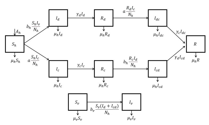
Figure 1: Compartement diagram for coendemic of COVID-19 and dengue.
Based on the above, we construct system of non-linear which describing the dynamic of coendemic COVID-19 and dengue disease, which is given by:
\[\begin{split} \frac{d\hat{S}_{h}(t)}{dt} &= A_{h} - b_{h} \frac{\hat{S}_{h}(t)\hat{I}_{v}(t)}{N_{h}(t)} - a \frac{S_{h}(t)\hat{I}_{c}(t)}{\hat{N}_{h}(t)} - \mu_{h}\hat{S}_{h}(t), \\ \frac{d\hat{I}_{d}(t)}{dt} &= b_{h} \frac{\hat{S}_{h}(t)\hat{I}_{v}(t)}{\hat{N}_{h}(t)} - \gamma_{d}\hat{I}_{d}(t) - \mu_{h}\hat{I}_{d}(t), \\ \frac{d\hat{R}_{d}(t)}{dt} &= \gamma_{d}\hat{I}_{d}(t) - a \frac{\hat{R}_{d}(t)\hat{I}_{c}(t)}{\hat{N}_{h}(t)} - \mu_{h}\hat{R}_{d}(t), \\ \frac{d\hat{I}_{dc}(t)}{dt} &= a \frac{\hat{R}_{d}(t)\hat{I}_{c}(t)}{\hat{N}_{h}(t)} - \gamma_{c}\hat{I}_{dc}(t) - \mu_{h}\hat{I}_{dc}(t), \\ \frac{d\hat{R}_{c}(t)}{dt} &= a \frac{\hat{S}_{h}(t)\hat{I}_{c}(t)}{\hat{N}_{h}(t)} - \gamma_{c}\hat{I}_{c}(t) - \mu_{h}\hat{I}_{c}(t), \\ \frac{d\hat{R}_{c}(t)}{dt} &= \gamma_{c}\hat{I}_{c}(t) - b_{h} \frac{R_{c}(t)\hat{I}_{v}(t)}{\hat{N}_{h}(t)} - \mu_{h}\hat{R}_{c}(t), \\ \frac{d\hat{I}_{cd}(t)}{dt} &= b_{h} \frac{\hat{R}_{c}(t)\hat{I}_{v}(t)}{\hat{N}_{h}(t)} - \gamma_{d}\hat{I}_{cd}(t) - \mu_{h}\hat{I}_{cd}(t), \\ \frac{d\hat{R}(t)}{dt} &= \gamma_{d}\hat{I}_{cd}(t) + \gamma_{c}\hat{I}_{dc}(t) - \mu_{h}\hat{R}(t), \\ \frac{d\hat{R}(t)}{dt} &= A_{v} - b_{v} \frac{\hat{S}_{v}(t)}{\hat{N}_{h}(t)}(\hat{I}_{d}(t) + \hat{I}_{cd}(t)) - \mu_{v}\hat{S}_{v}(t), \\ \frac{d\hat{I}_{v}(t)}{dt} &= b_{v} \frac{\hat{S}_{v}(t)}{\hat{N}_{h}(t)}(\hat{I}_{d}(t) + \hat{I}_{cd}(t)) - \mu_{v}\hat{I}_{v}(t), \\ \hat{N}_{h}(t) &= \hat{S}_{h}(t) + \hat{I}_{d}(t) + \hat{R}_{d}(t) + \hat{I}_{dc}(t) + \hat{I}_{c}(t) + \hat{R}_{c}(t) + \hat{I}_{cd}(t) + \hat{R}(t), \\ \hat{N}_{v}(t) &= \hat{S}_{v}(t) + \hat{I}_{v}(t), \end{split}\]
where all parameters are positive, \(\frac{d\hat{N}_h(t)}{dt}=A_h-\mu_h\hat{N}_h(t)\), and \(\frac{d\hat{N}_v(t)}{dt}=A_v-\mu_v\hat{N}_v(t)\). To reduce the dimension of System (1), we normalize variables by subtituting \(S(t) = \frac{\hat{S}(t)}{\hat{N}_h(t)}, I_d(t) = \frac{\hat{I}_d(t)}{\hat{N}_h(t)}, R_d(t) = \frac{\hat{R}_c(t)}{\hat{N}_h(t)}, I_c(t) = \frac{\hat{I}_c(t)}{\hat{N}_h(t)}, R_c(t) = \frac{\hat{R}_c(t)}{\hat{N}_h(t)}\). We assume that the total population \(\hat{N}_h(t)\) and \(\hat{N}v\) is constant, so we can represent \(A_h\) as \(\mu_h \hat{N}_h(t)\) and \(A_v\) as \(\mu_v \hat{N}v\). Further, to reduce the dimension of equation System (1) we normalize which are given as follow:
\[\frac{dS_{h}(t)}{dt} = \mu_{h} - b_{h}S_{h}(t)I_{v}(t) - aS_{h}(t)I_{c}(t) - \mu_{h}S_{h}(t), \frac{dI_{d}(t)}{dt} = b_{h}S_{h}(t)I_{v}(t) - \gamma_{d}I_{d}(t) - \mu_{h}I_{d}(t), \frac{dR_{d}(t)}{dt} = \gamma_{d}I_{d}(t) - aR_{d}(t)I_{c}(t) - \mu_{h}R_{d}(t), \frac{dI_{dc}(t)}{dt} = aR_{d}(t)I_{c}(t) - \gamma_{c}I_{dc}(t) - \mu_{h}I_{dc}(t), \frac{dI_{c}(t)}{dt} = aS_{h}(t)I_{c}(t) - \gamma_{c}I_{c}(t) - \mu_{h}I_{c}(t), \frac{dR_{c}(t)}{dt} = \gamma_{c}I_{c}(t) - b_{h}R_{c}(t)I_{v}(t) - \mu_{h}R_{c}(t), \frac{dI_{cd}(t)}{dt} = b_{h}R_{c}(t)I_{v}(t) - \gamma_{d}I_{cd}(t) - \mu_{h}I_{cd}(t), \frac{dR_{h}(t)}{dt} = \gamma_{d}I_{cd}(t) + \gamma_{c}I_{dc}(t) - \mu_{h}R_{h}(t), \frac{dS_{v}(t)}{dt} = \mu_{v} - b_{v}S_{v}(t)(I_{d}(t) + I_{cd}(t)) - \mu_{v}S_{v}(t), \frac{dI_{v}(t)}{dt} = b_{v}S_{v}(t)(I_{d}(t) + I_{cd}(t)) - \mu_{v}I_{v}(t),\] where \(N_h = 1\) and \(N_v = 1\). For the biological meaning, System (2) can be expressed as follow:
\[\frac{dX(t)}{dt} = \mathcal{F}(X(t)),\tag{3}\]
where \(X(t)=(S_h(t),I_d(t),R_d(t),I_{dc}(t),I_c(t),R_c(t),I_{cd}(t),R_h(t),S_v(t),I_v(t))^T\) and \(\mathcal{F}:\Omega\to\Omega\), with feasible region \(\Omega=\{X(t)\in\mathbb{R}\mid 0\leq x_i\leq 1,i=1,2,...,10\}\). The most convenient analytical procedure to state the positivity invariant is that investigating the euclidean dot product between outgoing normal vectors to the hyperplane boundaries of the non-negative \(2^{10}\)-hyperoctant of 10-dimensional Euclidean space and the vector fields of the system along these boundaries. Since the non-positive result of such dot product at all points lying on the coordinate hyperplanes exclude the origin, it will tell us that once the initial condition is taken inside the \(2^{10}\)-non negative hyperoctant, and if the trajectory touches any boundary afterward, then the trajectory will either return into the interior of this hyperoctant or remain on the boundary for all time and in the future. It follows that the region \(\Omega\) is positively invariant of System (2). The Parameters used in the model are described in Table 1.
3. ANALYSIS MODEL
In this section, we will discuss model analysis which includes: the basic reproductive ratio, the existence of an equilibrium point and the stability requirements of each equilibrium point.
3.1. Disease-free equilibrium and basic reproductive ratio
The disease-free equilibirum points are steady state solution of the proposed System (2), where there is no disease. We obtain the positive equilibirum human and mosquito population which we will denote by \(E_0\) and it is given by
\[E_0 = (S_h^0, I_d^0, R_d^0, I_{dc}^0, I_c^0, R_d^0, I_{cd}^0, R^0, S_n^0, I_n^0) = (1, 0, 0, 0, 0, 0, 0, 0, 0, 0).\]
| Parameter | Description | Unit | Value | Source |
|---|---|---|---|---|
| \(\mu_h\) | Host mortality rate | \(\frac{1}{day}\) | \(\frac{1}{65 \times 365}\) | [28] |
| \(\mu_v\) | Vector mortality rate | \(\frac{1}{day}\) | \(\frac{1}{14}\) | [29] |
| a | Transmission rate of COVID-19 infection | [0;1] | Assumed | |
| \(b_h\) | Transmission rate of Dengue infection from vector to host | \(\frac{\frac{1}{day}}{\frac{1}{day}}\) | [0;1] | Assumed |
| \(b_v\) | Transmission rate of Dengue infection from host to vector | \(\frac{1}{day}\) | [0;1] | Assumed |
| \(\gamma_d\) | Recovery rate of infected dengue | \(\frac{\frac{day}{d}}{day}\) | \(\frac{1}{10}\) | Assumed |
| \(\gamma_c\) | Recovery rate of infected COVID-19 | \(\frac{1}{day}\) | \(\frac{1}{14}\) | Assumed |
Table 1: Description parameters in System (2).
From the disease-free equilibirum, we use next generation matrix (NGM) to define the basic reproductive ratio \(\mathcal{R}_0\). The basic reproductive ratio is an average number of secondary infections caused by an infected individual that enter to the fully susceptible population throughout the period of infection. To construct NGM, we only notice the infected compartements \(I_{hd}\), \(I_{hdc}\), \(I_{hcd}\), \(I_{v}\) and we obtain the following transition Matrix \(\mathbf{V}\) and transition Matrix \(\mathbf{F}\) follow
\[\mathbf{F} = \begin{bmatrix} 0 & 0 & 0 & 0 & b_h \\ 0 & 0 & 0 & 0 & 0 \\ 0 & 0 & a & 0 & 0 \\ 0 & 0 & 0 & 0 & 0 \\ b_v & 0 & 0 & b_v & 0 \end{bmatrix} \text{ and } \mathbf{V} = \begin{bmatrix} \mu_h + \gamma_d & 0 & 0 & 0 & 0 \\ 0 & \mu_h + \gamma_c & 0 & 0 & 0 \\ 0 & 0 & \mu_h + \gamma_c & 0 & 0 \\ 0 & 0 & 0 & \mu_h + \gamma_d & 0 \\ 0 & 0 & 0 & 0 & \mu_v \end{bmatrix}.\]
We get next generation matrix as follow
\[\mathbf{NGM} = \mathbf{FV^{-1}} = \begin{bmatrix} 0 & 0 & 0 & 0 & \frac{b_h}{\mu_v} \\ 0 & 0 & 0 & 0 & \frac{b_h}{\mu_v} \\ 0 & 0 & 0 & 0 & 0 \\ 0 & 0 & \frac{a}{\gamma_c + \mu_h} & 0 & 0 \\ b_v & 0 & 0 & b_v & 0 \end{bmatrix}.\]
Using the method of Van den Driesche [30] and Diekmann [31], we know that \(\mathcal{R}_0\) is calculated by finding the spectral radius of NGM
\[\mathcal{R}_0 = \max\{\mathcal{R}_{0d}, \mathcal{R}_{0c}\},\tag{4}\] where
\[\mathcal{R}_{0d} = \frac{b_v b_h}{\mu_v (\gamma_d + \mu_h)}, \mathcal{R}_{0c} = \frac{a}{\gamma_c + \mu_h}.\]
3.2. Stability analysis of disease-free equilibrium
The disease-free equilibrium point \(E_0\) represents the absence of disease spread in a population, both COVID-19 and Dengue. Stability analysis at point \(E_0\) is given by finding that point on the Jacobian Matrix as follows
\[\text{[rumus tidak dapat ditampilkan dengan baik — lihat PDF asli]}\] and then, we have the characteristic equation of \(J(E_0)\) is
\[P_{0}(\lambda) = (\lambda + \mu_{h})^{4}(\lambda + \mu_{v})(\lambda + \gamma_{d} + \mu_{h})(\lambda + \gamma_{c} + \mu_{h})(\lambda + (\mu_{h} + \gamma_{c})(1 - \mathcal{R}_{0c}))\]\[(\lambda^{2} + (\mu_{v} + \gamma_{d} + \mu_{h})\lambda + \mu_{v}(\gamma_{d} + \mu_{h})(1 - \mathcal{R}_{0d}) = 0.\]
The eigenvalue of \(\lambda\) on \(P_0(\lambda)\) is negative when \(\mathcal{R}_0 < 1\), so the equilibrium point of \(E_0\) is locally asymptotically stable. We deduce that the point \(E_0\) is locally asymptotically stable if \(\mathcal{R}_0 < 1\) and a saddle point where \(\mathcal{R}_0 > 1\).
3.3. Boundary equilibrium
Boundary equilibrium or endemic equilibrium point of dengue is steady state solution of (2) where the disease of dengue persists in the population. The endemic equilibrium point of dengue is given by
\[E_d = \{S_h^*, I_d^*, R_d^*, 0, 0, 0, 0, 0, S_v^*, I_v^*\}\] (5)
where
\[S_h^* = \frac{\mathcal{R}_{0d}\mu_h + b_h}{\mathcal{R}_{0d}(b_h + \mu_h)}, I_{hd}^* = \frac{\mu_v \mu_h (\mathcal{R}_{0d} - 1)}{(b_h + \mu_h)b_v}, R_{hd}^* = \frac{\mu_v (\mathcal{R}_{0d} - 1)\gamma_d}{(b_h + \mu_h)b_v},\]\[S_v^* = \frac{(b_h + \mu_h)}{(\mathcal{R}_{0d}\mu_h + b_h)}, I_v^* = \frac{(\mathcal{R}_{0d} - 1)\mu_h}{\mathcal{R}_{0d}\mu_h + b_h}\] and \(E_d\) exist if and only if \(\mathcal{R}_{0d} > 1\).
The equilibrium \(E_c\) shows the diseases COVID-19 persists in the population with
\[E_c = (S_h^{**}, 0, 0, 0, I_c^{**}, R_c^{**}, 0, 0, 1, 0).\] (6)
where
\[S_h^{**} = \frac{1}{\mathcal{R}_{0c}}, I_c^{**} = \frac{\mu_h}{a} (\mathcal{R}_{0c} - 1), R_c^{**} = \frac{\gamma_c}{a} (\mathcal{R}_{0c} - 1).\]
We obtain conditions for the existence of positive endemic equilibrium COVID-19 when \(\mathcal{R}_{0c} > 1\).
3.4. Stability analysis of dengue boundary equilibrium
Further, we study now the stability of \(E_d\). Endemic equilibrium of dengue \(E_d\) is locally asymptotically stable when \(\mathcal{R}_{0d} > 1\) and \(\mathcal{R}_{0c} < \frac{b_v \mu_h - \mathcal{R}_{0d}(\gamma_d + \mu_h)}{b_v \mu_h - (\gamma_d + \mu_h)} = 1 + \frac{(\gamma_d + \mu_h)(1 - \mathcal{R}_{0d})}{b_v \mu_h - (\gamma_d + \mu_h)}\). For more details, see appendix A.
3.5. Stability analysis of COVID-19 boundary equilibrium
Using the linearization method, the characteristic polynomial of the Jacobian Matrix at point \(E_2\) is given as
\[P_c(\lambda) = (\lambda + \mu_h)^2 (\lambda + \gamma_c + \mu_h) ((\gamma_c + \mu_h) \lambda + \mu_h a) (\lambda + \mu_v) (\lambda + \gamma_d + \mu_h)\] \[(m_0 \lambda^2 + m_1 \lambda + m_2) (n_0 \lambda^2 + n_1 \lambda + n_2) = 0,\] (7)
m_2 = \mu_h(\gamma_c + \mu_h)^2 (\mathcal{R}_{0c} - 1),
n_0 = a(\gamma_c + \mu_h),
n_1 = a(\gamma_d + \mu_h + \mu_v)(\gamma_c + \mu_h),
n_2 = (\gamma_c + \mu_h)\mu_v(\gamma_d + \mu_h)(\mathcal{R}_{0c}\gamma_c + \mu_h\mathcal{R}_{0c} - \mathcal{R}_{0c}\gamma_c - \mu_h\mathcal{R}_{0c})
Based on Equation (7), we deduce that all eigenvalues are negative when \(\mathcal{R}_{0c} > 1\) and \(\mathcal{R}_{0d} < \frac{\mathcal{R}_{0c}(\gamma_c + \mu_h)}{\mathcal{R}_{0c}\gamma_c + \mu_h} = 0\)\(1 + \frac{\mu_h(\mathcal{R}_{0c} - 1)}{\mathcal{R}_{0c}\gamma_c + \mu_h}\). As a result, this condition reflects stability at the point \(E_c\). The bifurcation diagram in the plane-\(ab_h\) is shown in Figure 2 based on the stability conditions for the points \(E_d\) and \(E_c\).
3.6. Coendemic equilibrium
In this section, we are interest to find coendemic equilibrium that all subpopulation are not zero. It is shown implicitly by subpopulation \(I_v\) as follows
\[E_{co} = (S_h^{***}, I_d^{***}, R_d^{***}, I_{dc}^{***}, I_c^{***}, R_c^{***}, I_{cd}^{***}, R_c^{***}, S_v^{***}, I_v^{***})\] (8)
where
\[\begin{split} S_h^{***} &= \frac{\gamma_c + \mu_h}{a} = \frac{1}{\mathcal{R}_{0c}}, \\ I_d^{***} &= \frac{b_h \left(\gamma_c + \mu_h\right) I_v^{***}}{a \left(\gamma_d + \mu_h\right)}, \\ R_d^{***} &= \frac{I_v^{***} b_h \gamma_d \left(\gamma_c + \mu_h\right)^2}{a \left(\gamma_d + \mu_h\right) \left(\mu_h a - b_h \left(\gamma_c + \mu_h\right) I_v^{***}\right)}, \\ I_{dc}^{***} &= \frac{I_v^{***} b_h \gamma_d (\mu_h \left(a - \gamma_c - \mu_h\right) - b_h \left(\gamma_c + \mu_h\right) I_v^{***}\right)}{a \left(\gamma_d + \mu_h\right) \left(\mu_h a - b_h \left(\gamma_c + \mu_h\right) I_v^{***}\right)}, \\ I_c^{***} &= \frac{\mu_h \left(a - \gamma_c - \mu_h\right)}{a \left(\gamma_c + \mu_h\right)} - \frac{b_h \left(\mu_h + \gamma_c\right) I_v^{***}}{a \left(\gamma_c + \mu_h\right)}, \\ R_c^{***} &= \frac{\gamma_c \left(\mu_h \left(a - \gamma_c - \mu_h\right) - b_h \left(\gamma_c + \mu_h\right) I_v^{***}\right)}{\left(I_v^{***} b_h + \mu_h\right) \left(\gamma_c + \mu_h\right) a}, \\ I_{cd}^{***} &= \frac{I_v^{***} b_h \gamma_c \left(\mu_h \left(a - \gamma_c - \mu_h\right) - b_h \left(\gamma_c + \mu_h\right) I_v^{***}\right)}{a \left(b_h \left(\gamma_d + \mu_h\right) \left(\gamma_c + \mu_h\right) I_v^{***} + \mu_h \left(\gamma_d + \mu_h\right) \left(\gamma_c + \mu_h\right) I_v^{***}\right)}, \\ R_c^{***} &= \frac{I_v b_h \gamma_c \gamma_d \left(\gamma_c + a + \mu_h\right) \left(\mu_h \left(a - \gamma_c - \mu_h\right) - b_h \left(\gamma_c + \mu_h\right) I_v^{***}\right)}{a \left(\gamma_d + \mu_h\right) \left(\gamma_c + \mu_h\right) \left(I_v^{***} b_h + \mu_h\right) \left(\mu_h a - b_h \left(\gamma_c + \mu_h\right) I_v^{***}\right)}, \\ S_v^{***} &= \frac{a \mu_v \left(\gamma_d + \mu_h\right) \left(\gamma_c + \mu_h\right) \left(I_v^{***} b_h + \mu_h\right)}{b_h b_v \mu_h \left(b_h \left(\gamma_c + \mu_h\right) I_v^{***} + a \gamma_c + \gamma_c \mu_h + \mu_h^2\right)}. \end{split}\] and and the polynomial subpopulation \(I_v^{***}\) is
\[P(I_n^{***}) = q_0(I_n^{***})^2 + q_1 I_n^{***} + q_2 = 0, (9)\]
where \(q_0 = b_h^2 b_v \mu_h \left(\gamma_c + \mu_h\right) \mu_v\), \(q_1 = b_h \mu_v \left(\left(\gamma_c + \mu_h\right) \left(a\mu_v \left(\gamma_d + \mu_h\right) - b_h b_v \mu_h \left(\gamma_c + \mu_h\right) + b_v \mu_h^2 \left(\gamma_c + \mu_h\right) + a b_v \gamma_c \mu_h\right)\), \(q_2 = \mu_v \left(a\mu_h^2 \mu_v \left(\gamma_d + \mu_h\right) - b_h b_v \mu_h^2 \left(\gamma_c + \mu_h\right) - a \gamma_c \mu_h \left(b_h b_v - \mu_v \left(\gamma_d + \mu_h\right)\right)\right)\). To see that the polynomial \(\left(P(I_v^{***})\right)\) has one positive root \(I_v^{***}\), observe \(q_2\) with \(q_0 > 0\), and then the coefficient \(q_2\) is expressed as follows
\[q_2 = \mu_v^2 \mu_h(\gamma_c + \mu_h)(\gamma_d + \mu_h)(\mu_h(\mathcal{R}_{0c} - \mathcal{R}_{0d}) - \mathcal{R}_{0c}\gamma_c(\mathcal{R}_{0d} - 1)). \tag{10}\]
When \(\mathcal{R}_{0c} > 1\) and \(\mathcal{R}_{0d} > 1 + \frac{\mu_h(\mathcal{R}_{0c} - 1)}{\mathcal{R}_{0c}\gamma_c + mu_h}\), the Equation (10) becomes negative. Consider the following form \(I_c^{***}\), which is rewritten as follow
\[I_c^{***} = \frac{\mu_h}{a} (\mathcal{R}_{0c} - 1) - \frac{b_h}{a} I_v^{***}. \tag{11}\]
The form \(I_c^{***}\) is positive when \(I_v^{***} < \frac{\mu_h}{b_h}(\mathcal{R}_{0c} - 1)\) with \(a \neq 0\) and must be \(\mathcal{R}_{0c} > 1\) for \(I_v^{***} > 0\). This condition also applies to \(R_c^{***} > 0\) and \(I_{cd}^{***} > 0\). Moreover, the existences of \(R_d^{***}\), \(I_{dc}^{***}\), and \(R^{***}\) are obtained when \(I_v^{***} < \frac{\mu_h}{b_h}\mathcal{R}_{0c}\). Since \(\frac{\mu_h}{b_h}(\mathcal{R}_{0c} - 1) < \frac{\mu_h}{b_h}\mathcal{R}_{0c}\), we can conclude that there is coexistence of equilibrium points when \(\mathcal{R}_{0c} > 1\), \(\mathcal{R}_{0d} > 1 + \frac{\mu_h(\mathcal{R}_{0c} - 1)}{\mathcal{R}_{0c}\gamma_c + \mu_h}\), and \(0 < I_v^{***} < \min\{1, \frac{\mu_h}{b_h}(\mathcal{R}_{0c} - 1) = \frac{\mu_h b_v(\mathcal{R}_{0c} - 1)}{\mu_v \mathcal{R}_{0d}(\gamma_d + \mu_h)}\}\). Based on the conditions of existence and stability of the point \(E_0, E_1, E_2\) and the existence of the
Based on the conditions of existence and stability of the point \(E_0, E_1, E_2\) and the existence of the equilibrium coendemic \(E_3\), a bifurcation diagram in the plane-\(ab_h\) is given in Figure 2. For better visualization, we use parameter \(b_v = 0.1, \gamma_c = \frac{1}{21}, \gamma_d = \frac{1}{365}, \mu_v = \frac{1}{14}\) in Figure 2(a). However, we also use parameter values according to biological parameters with parameters \(b_v = 0.1, \gamma_c = \frac{1}{21}, \gamma_d = \frac{1}{365*70}, \mu_v = \frac{1}{14}\) in Figure 2(b). Figure 2(b) has a very small area III, but Figure 2(b) will be used for bifurcation diagrams in the numerical simulation session later according to its biological parameters.
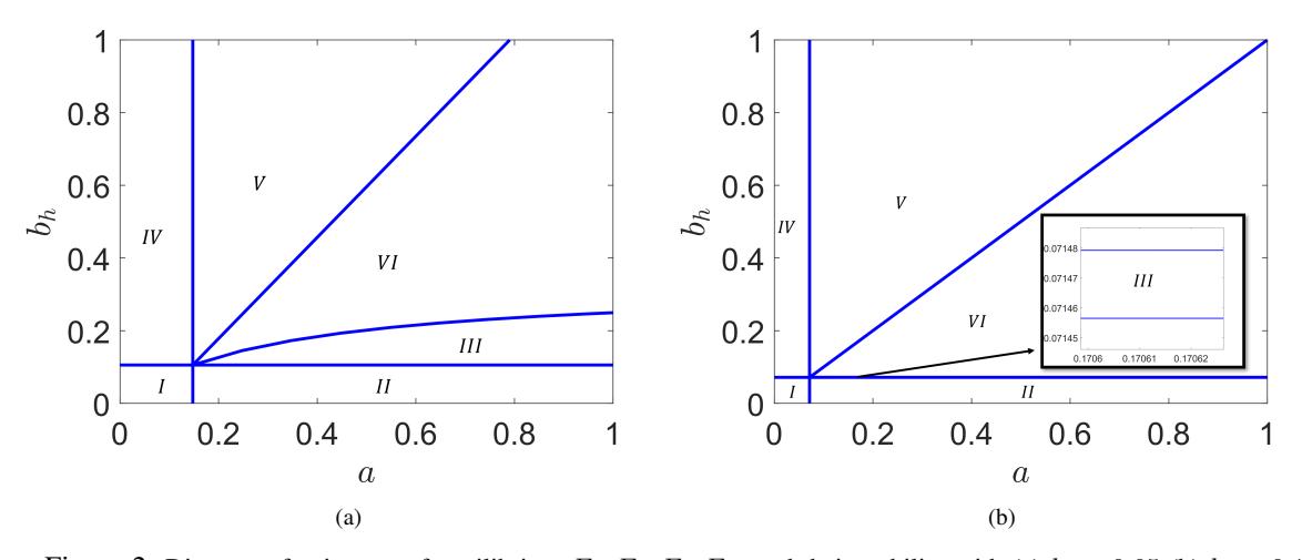
Figure 2: Diagram of existence of equilibrium \(E_0, E_d, E_c, E_{co}\) and their stability with (a) \(b_v = 0.05\) (b) \(b_v = 0.1\)
In Figure 2, there are six region of existence and stability equilibria:
\(I = \{E_0 \ exist \ and \ stable\},\\)
\(II = \{E_0 \text{ exist and unstable}, E_c \text{ exist and stable}\},\\)
\(III = \{E_0 \text{ exist and unstable}, E_c \text{ exist and stable}, E_d \text{ exist and unstable}\},\)
\(IV = \{E_0 \text{ exist and unstable}, E_d \text{ exist and stable}\},\)
\(V = \{E_0 \text{ exist and unstable}, E_c \text{ exist and unstable}, E_d \text{ exist and stable}\},\)
\(VI = \{E_0 \text{ exist and unstable}, E_c \text{ exist and unstable}, E_d \text{ exist and unstable}, E_{co} \text{ exist}\}.\)
4. NUMERICAL SIMULATION
In this session, numerical simulations are given to confirm the analytics that have been discussed in the previous session. In addition, bifurcation diagrams are provided to explain the stability of coendemic points which cannot be found analytically. First, we consider all parameter biology in Table 1 and also parameter \(b_v = 0.1\). In Figure 3, we fix parameter a = 0.4 and we plot equilibrium \(I_d\) and \(I_c\) at points \(E_c\) (in blue),
\(E_d\) (in red) and \(E_{co}\) (in magenta) against parameter \(b_h\). This result is consistent with Figure 2(b), when we set a=0.4 and vary the parameter \(b_h\), then there are three regions that are traversed, namely region II (\(E_c\) stable), region VI (existence of point \(E_{co}\)), and region V (\(E_d\) stable). In more detail, Figure 3(a) shows that when \(b_h < 0.07145652782\) (condition \(R_d < 1\)), point \(E_c\) exists and is unstable, and point \(E_d\) and \(E_{co}\) do not exist. Furthemore, when \(b_h^* < b_h < b_h^{*****}\) (see in Figure 3), point \(E_c\) is stable and point \(E_d\) is not stable. An interesting thing happens when \(b_h^{*****} < b_h < b_h^{**}\), there are two points, \(E_d\) and \(E_{co}\). In this state, the point \(E_d\) is unstable. In contrast to the point \(E_{co}\), it is unstable when \(b_h^{***} < b_h < b_h^{*****}\), and others are stable under this condition. The stability of this \(E_{co}\) point is described in more detail in Figure 4.
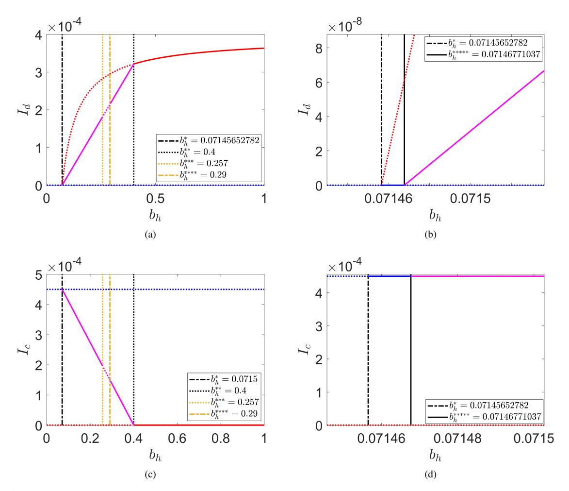
Figure 3: Bifurcation diagram (a) and (c) equilibrium \(I_d\) and \(I_c\) against parameter \(b_h\), respectively, (b) and (d) equilibrium \(I_d\) and \(I_c\) against parameter \(b_h\) version zoom (a) and (c), respectively, for equilibria \(E_c\) (in blue), \(E_d\) (in red), and \(E_{co}\) (in magenta). Stable equilibrium is marked solid curve and unstable equilibrium is denoted by dashed curve.
We use parameter \(b_v=0.1, \gamma_c=\frac{1}{21}, \gamma_d=\frac{1}{365*70}, \mu_v=\frac{1}{14}, a=0.4\) in Figure 4. Figure 4 describes the change in the coendemic equilibrium value of \(I_{cd}^{***}\) and \(I_{dc}^{***}\) against parameter \(b_h\). We use Matcont package in Matlab for simulating bifurcation diagram. In Figure 4, the unstable point has a pair of complex eigenvalues, one of them positive real and non-zero imaginary part, and the others have negative real parts. It is unstable when \(0.257 < b_h < 0.29\). There are two Hopf bifurcation points where the real part is zero and the imaginary part is not zero, when \(b_h=0.257\) and \(b_h=0.29\). We denote these two points as \(H_1\) and \(H_2\), respectively. When \(b_h\in(0.257;0.29)\), they are stable with a pair of complex eigenvalues that real part is negative and the imaginary part is not zero, and the other is negative. Limit cycle exists and is stable when \(0.257 < b_h < 0.29\). Figures 4(b) and 4(d) show equilibrium and amplitude when the limit cycle exists. The maximum peak of the limit cycle is \(I_{dc}^{***}=8*10^{-4}\) when \(b_h=0.258\) and \(I_{cd}^{***}=13*10^{-5}\) at the time of \(b_h=0.26\).
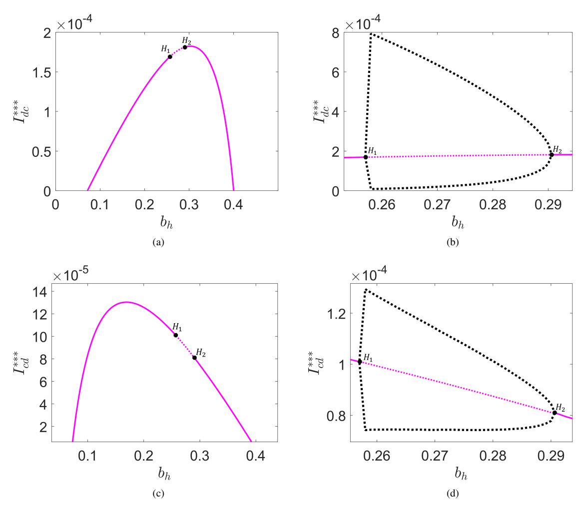
Figure 4: Bifurcation diagram for coexistence equilibrium (a) and (c) \(I_{dc}^{***}\) and \(I_{cd}^{***}\) against \(b_h\), respectively, (b) and (d) diagram bifurcation zoom version with amplitude. The black dashed curve indicates the maximum and minimum of the periodic solution of System (2). Point \(H_1\) and \(H_2\) label the first Hopf bifurcation and the second Hopf bifurcation.
Figure 4 shows that coendemic conditions exist when the dengue transmission rate from the vector to the host is between 0.05 and 0.38. Coendemic conditions always exist for \(t \to \infty\) for the transmission rates of \(b_h \in (0.05; 0.257)\) and \(b_h \in (0.29; 0.38)\) with a population size infected with dengue after recovering from COVID-19 (population size of infected with COVID-19 after recovering from dengue) is constant. However, at the time of \(b_h \in (0.258; 0.29)\), the population sizes of \(I_{cd}\) and \(I_{dc}\) are not constant but have a period. This condition provides an important warning to us that the maximum number of the infected population must be considered with the number of hospital facilities stock.
The amplitude in Figure 6 describes the difference between the maximum and minimum \(I_{cd}\) and \(I_{dc}\) when a limit cycle exists. Increasing the amplitude indicates a large maximum and minimum distance. Figure 6 shows that the amplitude of \(I_{dc}\) is greater than the amplitude of \(I_{cd}\). In Figure 5(a), when \(b_h=0.259\), the amplitude of \(I_{dc}\) is 0.00078. This means \(\frac{78}{10000}\) of the total population and this number is high. This value is quite large for the number of population who experience secondary infection with COVID-19 after recovering from dengue. We also display the period of the limit cycle in Figure 5. The result is that the average period is about 7-9 years. This time is long enough for one period of infection of one population.
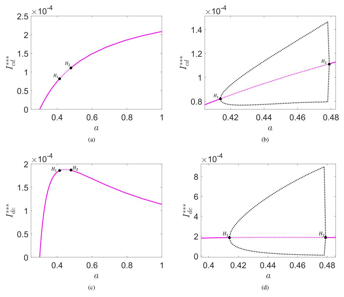
Figure 5: Bifurcation diagram for coendemic equilibrium (a) and (b) \(I_{cd}^{***}\) and \(I_{dc}^{***}\) against parameter a, respectively, and (b) and (d) diagram bifurcation zoom version with amplitude. The black dashed curve indicates the maximum and minimum of the periodic solution of System (2).
In Figure 5, we set the parameter \(b_v=0.1, \gamma_c=\frac{1}{21}, \gamma_d=\frac{1}{365*70}, \mu_v=\frac{1}{14}, b_h=0.1\). We also show bifurcation diagram of the coendemic equilibrium point \(I_{cd}^{***}\) and \(I_{dc}^{****}\) against the parameter a. The existence of a limit cycle between the two Hopf bifurcation points, \(H_1\) and \(H_2\), can also be found by varying parameter a and they are in a=0.414 (\(H_1\)) and in a=0.479 (\(H_2\)), while others are stable. In contrast to Figure 4, Figure 5 shows that the maximum is greatest when it approaches \(H_2\). In Figure 4 and Figure 5, the maximum \(I_{dc}^{***}\) is higher than the maximum \(I_{cd}\). It means that the number of the population of COVID-19 after recovering from dengue is always higher than the number of population infected with dengue after recovering from COVID-19. Another interesting thing is shown in Figure 6. The period in Figure 6(a) is higher with a variation of parameter \(b_h\) than in Figure 6(b) (variation of parameter a). Figure 7 shows the limit cycle (in red), and phase portrait with initial values from inside and outside the limit cycle (in blue).
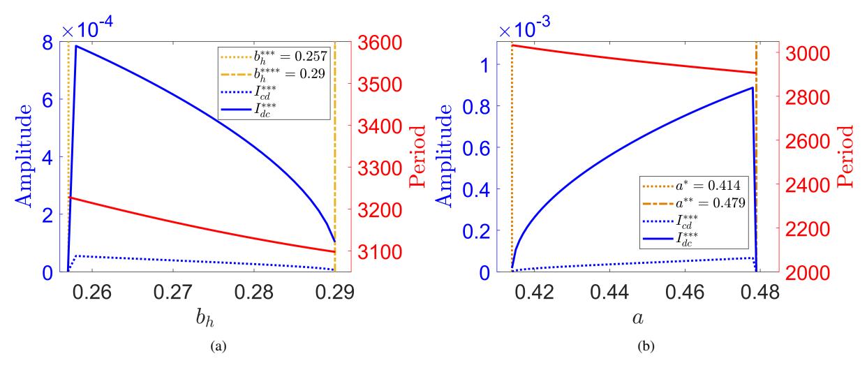
Figure 6: Amplitude and period solution periodic \(I_{cd}^{***}\) and \(I_{dc}^{***}\) with varied (a) parameter \(b_h\) and (b) parameter a.
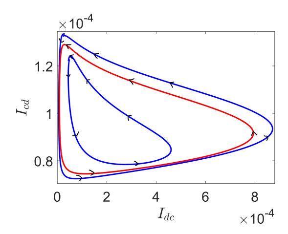
Figure 7: Phase portrait \(I_{cd}\) against \(I_{dc}\) with parameter \(b_v = 0.1, \gamma_c = \frac{1}{21}, \gamma_d = \frac{1}{365*70}, \mu_v = \frac{1}{14}, b_h = 0.258, a = 0.4\).
5. CONCLUSION
In this paper, we have constructed a coendemic model describing transmission of two pathogens leading to a coendemic phenomenon for dengue and COVID-19 disease. We divided the population into ten compartments: susceptible, infected by dengue, infected by COVID-19, infected by COVID-19 in secondary infection, infected by Dengue in secondary infection recovered from Dengue, recovered from Covid, and recovered from two pathogens. Four equilibria are discussed: pathogen-free equilibrium, two boundary equilibria (single
endemic Dengue, and single endemic COVID-19), and coendemic equilibrium. Basic reproductive ratio \(\mathcal{R}_0\) is obtained, followed by the existence of the boundary equilibria when \(\mathcal{R}_0 > 1\).
For the coendemic case, we use numerical simulation to determine its stability. Two Hopf bifurcations are found in the coendemic point bifurcation diagram with respect to parameter \(b_h\). The existence of a limit cycle is found between the two Hopf points. The limit cycle periods grow and reach the maximum value and decrease as the coendemicrates increase. Beyond the second Hopf point, the coexistence equilibrium is stable.
ACKNOWLEDGEMENT
HF respectfully acknowledges the financial assistance granted by the Ministry of Research and Technology of Indonesia through the PMDSU Program [grant No. 1511/E4.4/2015]. Part of this work of ES, NN, and HF are funded RistekDikti Doctor Grant 2021 [grant no. 111/IT1.C02/TA.00/2021 and 120L/IT1.C02/TA.00/2021].
APPENDIX A. STABILITY OF \(E_d\)
First, we evaluate point \(E_d\) in Matrix Jacobian and characteristic equation \(P_d(\lambda)\) is given by
\[P_d(\lambda) = (\lambda + \mu_h)^2 (\lambda + \mu_v)(\lambda + \gamma_d + \mu_h)(\lambda + \gamma_c + \mu_h)((b_v \mu_h + \gamma_d \mu_v + \mu_h \mu_v) \lambda + b_h b_v \mu_h + b_v \mu_h^2)(k_1 \lambda + k_2)(l_1 \lambda^3 + l_2 \lambda^2 + l_3 \lambda + l_4) = 0.\] where \[k_1 = -b_v (\mu_h + b_h)\] \[k_2 = a\mu_v (\gamma_d + \mu_h) - b_h b_v (\gamma_c + \mu_h) + b_v \mu_h (a - \gamma_c - \mu_h)\] \[= (\gamma_c + \mu_h)\mu_h b_v (\mathcal{R}_{0c} - 1) - (\gamma_c + \mu_h)(\gamma_d + \mu_h)(\mathcal{R}_{0c} - \mathcal{R}_{0d})\] \[l_1 = (\mu_h + b_h) (\gamma_d + \mu_h) (\mu_h (\mu_v + b_v) + \gamma_d \mu_v),\] \[l_2 = (2b_v + \mu_v) \mu_h^4 + ((3b_v + \mu_v)b_h + 3\gamma_d (\mu_v + b_v)) \mu_h^3\] \[+ \left(b_h^2 b_v + \left((4b_v + 3\mu_v) \gamma_d + (\mu_v + b_v)^2\right)b_h + \gamma_d^2 (b_v + 3\mu_v)\right) \mu_h^2\] \[+ \gamma_d \left(b_h^2 b_v + ((b_v + 3\mu_v) \gamma_d + 2\mu_v (\mu_v + b_v))b_h + \mu_v \gamma_d^2\right) \mu_h + b_h \mu_v \gamma_d^2 (\mu_v + \gamma_d),\] \[l_3 = \mu_h \mu_v (\gamma_d + \mu_h) (\mathcal{R}_{0d} - 1) \left(b_v \gamma_d \mu_h + 2b_v \mu_h^2 + \gamma_d^2 \mu_v + 3\gamma_d \mu_v \mu_h + \mu_v \mu_h^2\right) + b_v \mu_h^4 \mu_v\] \[+ b_v \gamma_d \mu_h^3 \mu_v + \gamma_d^2 \mu_h^2 \mu_v^2 + \gamma_d \mu_h^3 \mu_v^2 + b_v \mu_h (b_h^2 b_v \mu_h + b_h^2 \gamma_d^2 + 2b_h^2 \gamma_d \mu_h + b_h^2 \gamma_d \mu_v\] \[+ b_h^2 \mu_h^2 + b_h^2 \mu_h \mu_v + 2b_h \gamma_d^2 \mu_h + 4b_h \gamma_d \mu_h^2 + 2b_h \mu_h^3 + b_h \mu_h^2 \mu_v + \gamma_d^2 \mu_h^2 + 2\gamma_d \mu_h^3 + \mu_h^4),\] \[l_4 = \mu_h (\gamma_d + \mu_h)^2 (\mu_h (\mu_v + b_v) + \gamma_d \mu_v) (\mu_h + b_h) \mu_v (\mathcal{R}_{0d} - 1).\] Observe that \(l_1, l_2, l_3, l_4 > 0\) when \(\mathcal{R}_{0d} > 1\). Further, it can be seen that
\[l_2 l_3 > (\gamma_d + \mu_h)^3 (b_v \mu_h + \gamma_d \mu_v + \mu_h \mu_v)^2 (\mu_h + b_h)^2 \mu_h \mu_v (\mathcal{R}_{0d} - 1) = l_1 l_4.\]
Using Routh-Hurtwitz criteria, the roots of characteristic polynomial of \(P_d(\lambda)\) have negative real part when \(\mathcal{R}_{0d}>1\) and \(\mathcal{R}_{0c}<\frac{b_v\mu_h-\mathcal{R}_{0d}(\gamma_d+\mu_h)}{b_v\mu_h-(\gamma_d+\mu_h)}=1+\frac{(\gamma_d+\mu_h)(1-\mathcal{R}_{0d})}{b_v\mu_h-(\gamma_d+\mu_h)}\). Therefore the endemic equilibrium \(E_d\) is locally asymptotically stable.