

1. INTRODUCTION
In December 2019, first positive case of coronavirus was identified in the city of Wuhan, Hubei, China [1]. It follows on January 13th, 2020, the first case outside China was reported and the disease rapidly spread globally to at least 220 country in early 2020 [2]. As of January 30,2020, Coronavirus disease (COVID-19) was reported as a public health crisis of international attention [2].
Indonesia is also one of the countries affected by coronavirus infection. It reported its first confirmed cases of COVID-19 on March 2, 2020, with two people was tested positive [3]. As of March 31, 2020, Indonesia recorded 1,528 cases, spread across 31 provinces, with nearly 85% of cases occurring in Java [4]. Considering the advancing threat of COVID-19, it is indispensable to use real-time infodemiology data to monitoring the outbreak and people behaviour in responding to the epidemic. As the internet has grown an essential source for information seeking both for health information and non-health information, it can be employed as a "alternate" indicator of disease awareness in in the circumstances of public attention [6].
One of the most favourite infodemiology resources is Google Trends that has been extensively utilised in medicine and health for the prediction and research of epidemics and disease. Through Google Trends, it is possible to access the query share of a particular searches for a user specified search term among all searches. That such as data is often called as relative search volume (RSV), which the proportion of a particular search pattern according to specified keywords for a given time period and location, normalised by the highest query of that search term [7]. These approaches have been suggested to be necessary for the studying and forecasting of outbreaks and pandemics, such as dengue [8], COVID-19 [9], [10], [11], and influenza [12].
In this paper, Google Trends data on specific keywords on the topic of "Covid-19" are assess to explore the relationship between cases in Java Province, Indonesia with online interest in the outbreak of the disease. First, a lag correlation method is applied to analyse the linear-relation between RSV data and COVID-19. In this result, correlation is inclined to describe the synchronisation between each pair data of Covid-19 cases and RSV data [13]. However, the disadvantage of this approach is that it does not describe causal relation between two time series data. Second, the application of Granger causality in the second method will be
*Corresponding author
produced the causality relation in time series data. Thus, the relation between Covid-19 cases and Google Trend data can be analysed whether they occur due to a common cause or chance, or due to cause-effect relations.
The rest of the paper is structured as follows. The Description of data section details the data collection procedure of Google trend data and New Covid-19 Cases. The section method consists the statistical analysis tools and methods. The Results section consists of the correlation analysis and Granger causality result between Covid-19 time series data and Google Trend data. The conclusion section presents the main findings of this work, along with the limitations of this paper and future research suggestions.
2. DESCRIPTION OF DATA
2.1. Google Trend Data
Google Trends (GT) data have been impacted extensively for investigating care-seeking patterns and helath information using trends on either Google News, Web search, or YouTube [7]. Since the release, these data became commonly used in epidemiology when Ginsberg et al. utilize it as a valuable tool to predict influenza epidemics especially for large population areal [14]. On advancement, in 2014, it is reported that 60% of Google Trends research was focused human behavior and infectious diseases [15].
To access GT data, a user scans Google search outcome for a fraction of passages for a particular term ("keyword" or "search term") according to defined time frame and a specific area or location and. The keyword can be in the form of a single word or a phrase, and certain of these can be merged into a single search trend data which functions like "OR" by joining with the keyword with a "+". Then, the search result provides Google Trends Index for the keywords used, which represents relative search volume (RSV) for each query on a scale from 0 to 100, where 100 represents the highest point [16].
In this study, we regained GT data on the five commonly online searched keywords that Indonesians might have used associated to the response of COVID-19. The keywords or phrase that were carried out for the analysis were the the Indonesian equivalents to the English keywords "Covid" (Indonesian:"Covid"), "Covid-19" (Indonesian: "Covid-19"), "pandemic" (Indonesian:"pandemi"), "Corona" (Indonesian:"Corona"), "coronavirus disease 2019" (Indonesian: "penyakit korona virus 2019"). The focus of our analysis is only on Java in 6 different provinces: Banten, Special Capital Region of Jakarta, West Java, Central Java, Yogyakarta Special Region, and East Java with time limit from June 14, 2020, until February 14, 2021. For each province, Figure 1 shows plot of daily GT data in blue color for each province.
2.2. New COVID-19 Cases
A confirmed positive case of COVID-19 is specified as one in which the patient have positive positive test result of the reverse transcriptase-polymerase chain reaction (RT-PCR) test. As of February 14, 2021, the cumulative COVID-19 cases in Indonesia reached 1.22 million cases, and it was spread over 34 provinces [4]. It was reported that the majority of the cases occurred in Java (Table 1 which was almost 67% of the total cases. Thus, we narrowed our analysis to focus only on the Java area. There are six provinces in total on Java, Indonesia. The daily time series data is collected of each province and represents in Figure 1.
The number of daily new confirmed cases in Indonesia were obtained for the period June 14, 2020,
Table 1: Frequency of cumulative COVID-19 case in the provinces of Java. The cumulative data of COVID-19 cases was from the date of the first confirmed COVID-19 case in the respective province until February 14, 2021.
| Province | COVID-19 cumulative cases |
|---|---|
| Banten | 27145 |
| Special Capital Region of Jakarta | 315513 |
| West Java | 175003 |
| Central Java | 141437 |
| Yogyakarta Special Region | 25033 |
| East Java | 122375 |
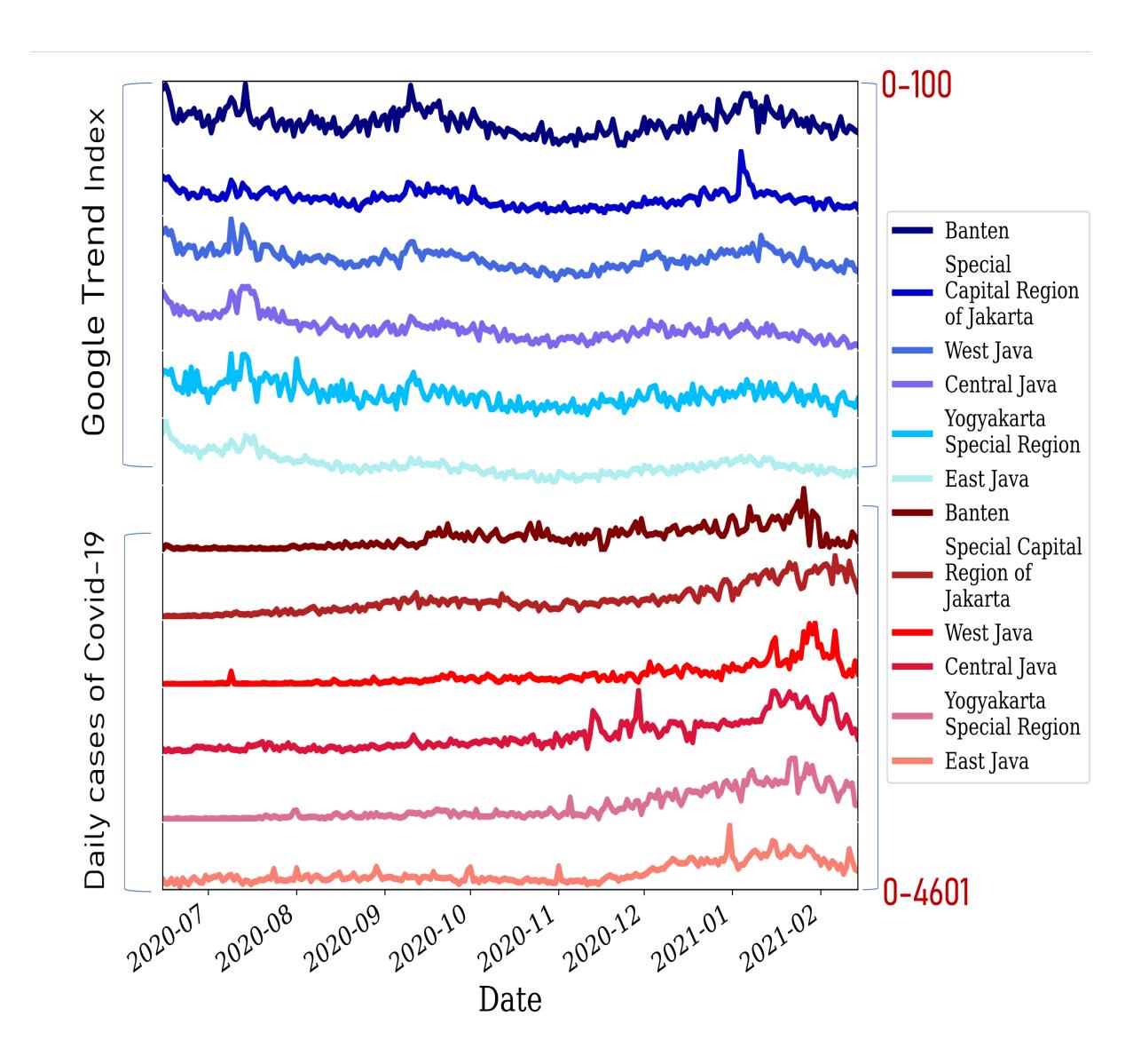
Figure 1: Time series plots of Google Trend relative search volume (RSV) in Web search, YouTube search, and News search.
until February 14, 2021 from https://covid19.go.id/peta-sebaran. The data were derived from this upstream repository maintained by the Health Ministry of Indonesia.
3. METHOD
3.1. Cross-Correlation Function
The CCF between two different time series helps to understand the nature of the relationship and how they are correlated in time [5]. Denoting two time series data by yt and xt, a simple method to examine a possible linear association between the processes is by using cross-correlation function (CCF). Since the series yt may be related to past lags of the series xt, CCF can also be used to identify the relationship with different time-shifted data.
The sample CCF ρˆxy(k) is accounted as the set of sample correlation between time series yt and different time-shifted time series xt+k for k = 0, ±1, ±2, .... For each possible lag number k, it is defined as
\[\hat{\rho}_{xy}(k) = \frac{1}{\hat{\sigma}_x \hat{\sigma}_y(n-k)} \sum_{t=1}^{n-k} (x_t - \bar{x})(y_t - \bar{y}), \tag{1}\] with n is the number of observations, σˆx, σˆy are the sample standard deviations of the processes, and x¯),(¯y are the mean estimation of time series data [18]. Noted that ρˆxy(k) ̸= ˆρxy(−k). Therefore, it is necessary to really pay attention to which variable is the response and which variable is the predictor.
To assure that the observed correlations do not happen by a chance, a significance test should be performed. To test the null hypothesis H0 : ρxy(k) = 0 of no cross-correlation at time lag k, it typically use t-statistic with
\[t_{xy}(k) = \sqrt{n}\hat{\rho}_{xy}(k) \tag{2}\]
at a α significance level [5] and and resulted (−tα/2/ √ n, tα/2/ √ n) for 100(1 − α)% confidence band (CB) This standard inferences are only valid for mutually independent bivariate/multivariate data and their size can be significantly distorted otherwise, in particular, by heteroscedasticity. The robust method [18] can be applied to avoid invalidated CCF by allowing testing under more general settings, e.g., heteroscedasticity and dependence in each series and mutual dependence across series. Rather than use Equation (2) to calculate the t-statistic, the robust procedures take t-statistic with
\[\tilde{t}_{xy}(k) = \frac{\sum_{t=k+1}^{n} e_{xy,tk}}{\sqrt{\sum_{t=k+1}^{n} e_{xy,tk}^{2}}},\] (3)
with exy,tk = (xt+k −x¯)(yt −y¯) and resulted (−tα/2 ρˆxy(k) t˜xy(k) , −tα/2 ρˆxy(k) t˜xy(k) ) for 100(1−α)% confidence band (CB).
3.2. Granger Causality
Granger causality is a method that was developed to enhance the predictability of the effect variable when the causal (driving) variable is followed. The use of this method is based on two assumptions: 1) cause befalls before effect and 2) the knowledge of the cause give information about the effect [21]. Indicating the cause and the effect variables by two stationary time series xt and yt, respectively, if the reduction in the autoregressive prediction error variance of time series yt at present occurs by the inclusion of past measurements from xt, then it is claimed to have a causal influence [22]. In implementation, it can be shown by estimating of multivariate vector autoregressions (MVAR) with lag p as follows
\[y_{t} = C + \sum_{i=1}^{p} \delta_{i} y_{t-i} + \epsilon_{y-t}\] \[y_{t} = C_{1} \sum_{i=1}^{p} (\delta_{i} y_{t-i} + \beta_{i} x_{t-i}) + \eta_{y_{t}}.\] \[(4)\]
According to Equation (4), the existence of Granger causality from xt to yt can be evidenced if
\[var(\epsilon_t) = var(y_t - \hat{y}_t y_{0:t-1}) > var(y_t - \hat{y}_t | x_{0:t-1}, y_{0:t-1}) = var(\eta_t).\] (5)
One might efficiently investigate this relationship based on hypothesis test using F test procedure to inquire for significant effects of past values of xt on the present value of yt [23]. let, the null and alternative hypotheses are defined as follows
\[H_0: \qquad \beta_1=\beta_2=...=\beta_p=0 \\ H_1: \quad \text{At least there is } \beta_i \text{ is not zero for } i=1,2,..,p\]
which the null hypothesis, H0 represents the absence of causality between time series and the alternative hypothesis corresponds to the significant influence of some past values of xt on time series yt but not certainly for all. In other direction, the causality from yt to xt can be shown as
\[x_{t} = D + \sum_{i=1}^{q} \gamma_{i} x_{t-i} + \epsilon_{x_{t}}\] \[x_{t} = D_{1} + \sum_{i=1}^{q} (\gamma_{i} x_{t-i} + \lambda_{i} y_{t-i}) + \eta_{x_{t}}.\] \[(7)\]
With same procedure, the hypothesis test is applied by using F test, the null and alternative hypotheses to test the significant effect of yt on the equation (7) is defined as
\[H_0:\] \(\lambda_1 = \lambda_2 = ... = \lambda_q = 0\) (8)
\(H_1:\) At least there is \(\lambda_i\) is not zero for \(i = 1, 2, ..., q\).
With significant level α, if H0 is rejected for both F tests as explained in (6) and (8) then there are two directions of Granger causality between the time series (xt influence yt and vice versa). However, if only H0 from hypothesis testing (6) is rejected, it concludes that there is only one direction of causality, e.g. xt Granger cause yt and vice versa if the hypothesis (8) is rejected.
4. RESULT
4.1. Break-Point of Time Series Data
Successive captures of daily Covid-19 cases throughout the observation period and google trend data are presented in Figure 1. In many applications, it is reasonable to assume that for different ranges of COVID-19 daily cases, there may be different linear relationships occur with GT data. In these cases, a single crosscorrelation value may not provide an adequate description over the observation period. The point at which the coefficient shifts from one stable relationship to a different one is called the breakpoints [20]. Thus, before the cross-correlation coefficient is calculated for every province, m breakpoints will be checked first, produced m + 1 segments in our time series data. The computation was processed using R package strucchange to obtain the segments data (daily Covid-19 cases for each province with google trend data). Figure 2 depicts several segments to illustrate the relationship between incidence data and Google Trend data.
The result in Figure 2 indicates that during 7 months period, there are 3 to 5 times changes in the relationship between COVID-19 daily cases and the behavioral response of the Indonesian people in seeking information on topics related to it via online. Uniquely, some of the periods of change are found in relatively the same time period in each province. For example around November 2020, every province was discovered to experience changes in behavior between COVID-19 daily cases and GT data. The second break-point is that 5 of 6 province encountered it around January 2021. Hence, rather then only calculated single cross-correlation coefficient, here, it computed per break-point time period.
4.2. Lag Cross Correlation Analysis
According to the outcome in subsection 4.1, we evaluate the lag CCF between GT data and new cases of COVID-19 for each period of the provinces in Java. We examine the CCF for lag in range [−7, 7] in which the result shows in Table 2. Using the significance level of 5%, the correlation values for each province are not proven to be significant in period 1. Conversely, the CCF values begin significantly in periods 2 and 3. It also reveals that each period has different characteristics of CCF value in each province. For example, Special capital region of Jakarta has negative linear relationship between GT data and new cases of COVID-19 in period 5 (except for lag -7), but have completely positive linear relationship in periods 2 and 3. It reveals that it is impossible to only get a single value of CCF through one set of time series data.
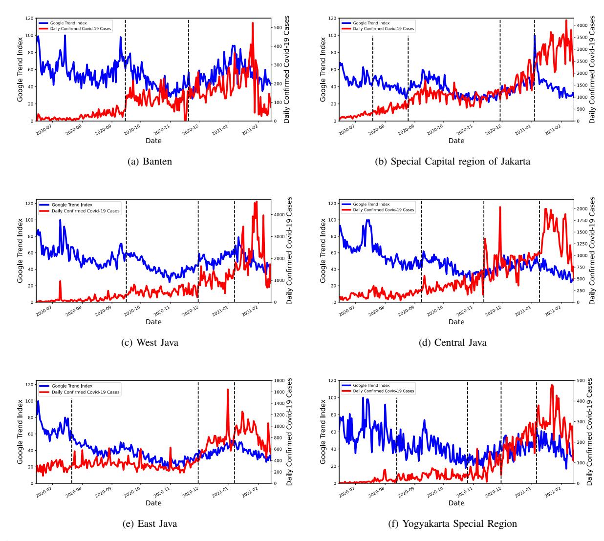
Figure 2: Segment data in time series of a linear relationship between COVID-19 daily cases and Google Trend Data for each province in Java.
In Yogyakarta, correlation between the GT data in terms of the keywords and the daily new laboratoryconfirmed COVID-19 cases in reaches the maximum during the lag periods of -7 days of GT data in period 3 with xyˆ = 0.545. For Banten, Jakarta and West Java, the maximum correlations reach in period 2 with lag period -3 days with ρˆxy = 0.575 , with lag period 7 days with ρˆxy = 0.545, and lag period -4 with ρˆxy = 0.381, respectively. In other hand, Central Java and East Java reach the maximum correlation in period 4 with lag -1 for both provinces with value 0.579 and 0.597, respectively. Here, we found that although the correlation in each period of time is not strong enough, the the synchronisations between GT data and Covid-19 cases in each province are different, regardless the behaviour of outbreak is the same. In addition, the East Java province is found, the highest lag-correlation relatively does not change much in each period. This is different from what happen in Yogyakarta province, the lag-correlation in second period is very weak, (almost with no linear-correlation), but in last period, the correlation is getting stronger.
Table 2: Lag correlation coefficients between Google Trends data and New confirmed cases of COVID-19 in Java, June 14, 2020 to February 14, 2021. Black dash line and red dash line indicates the 95% confidence band and robust confidence band, respectively.
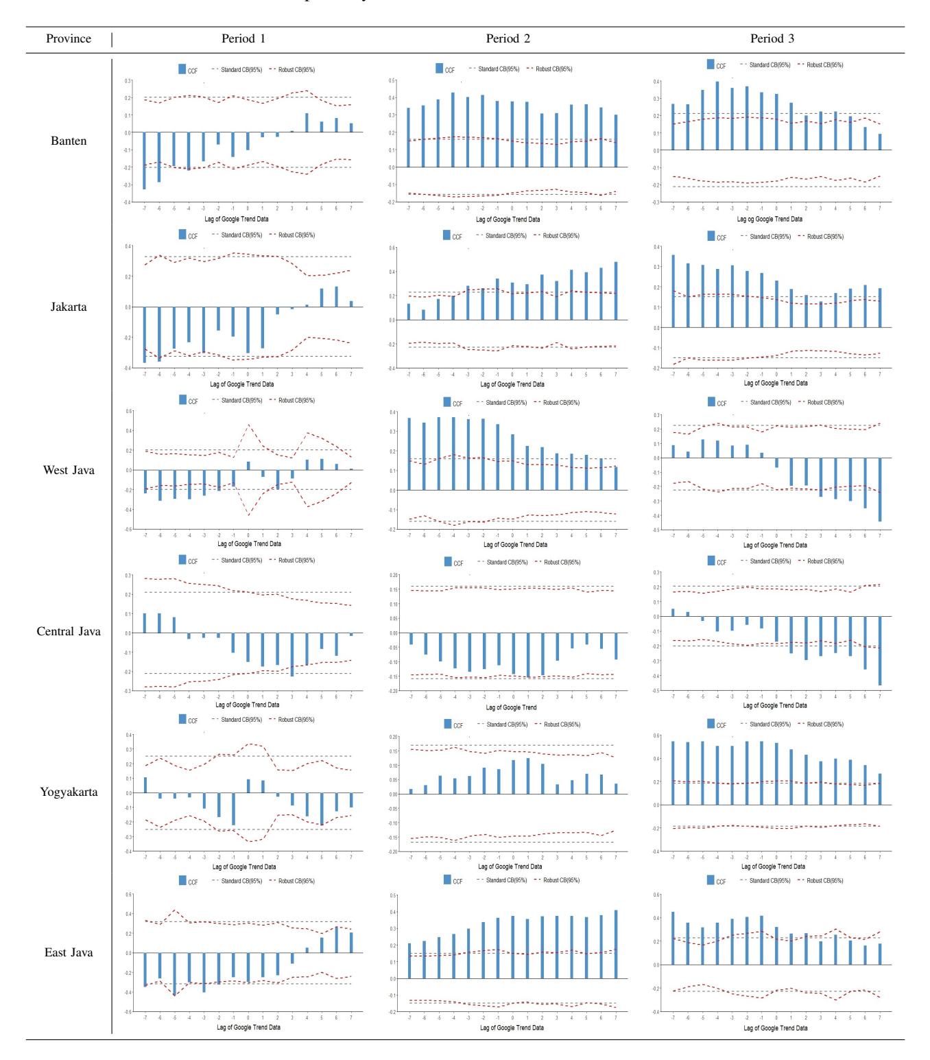
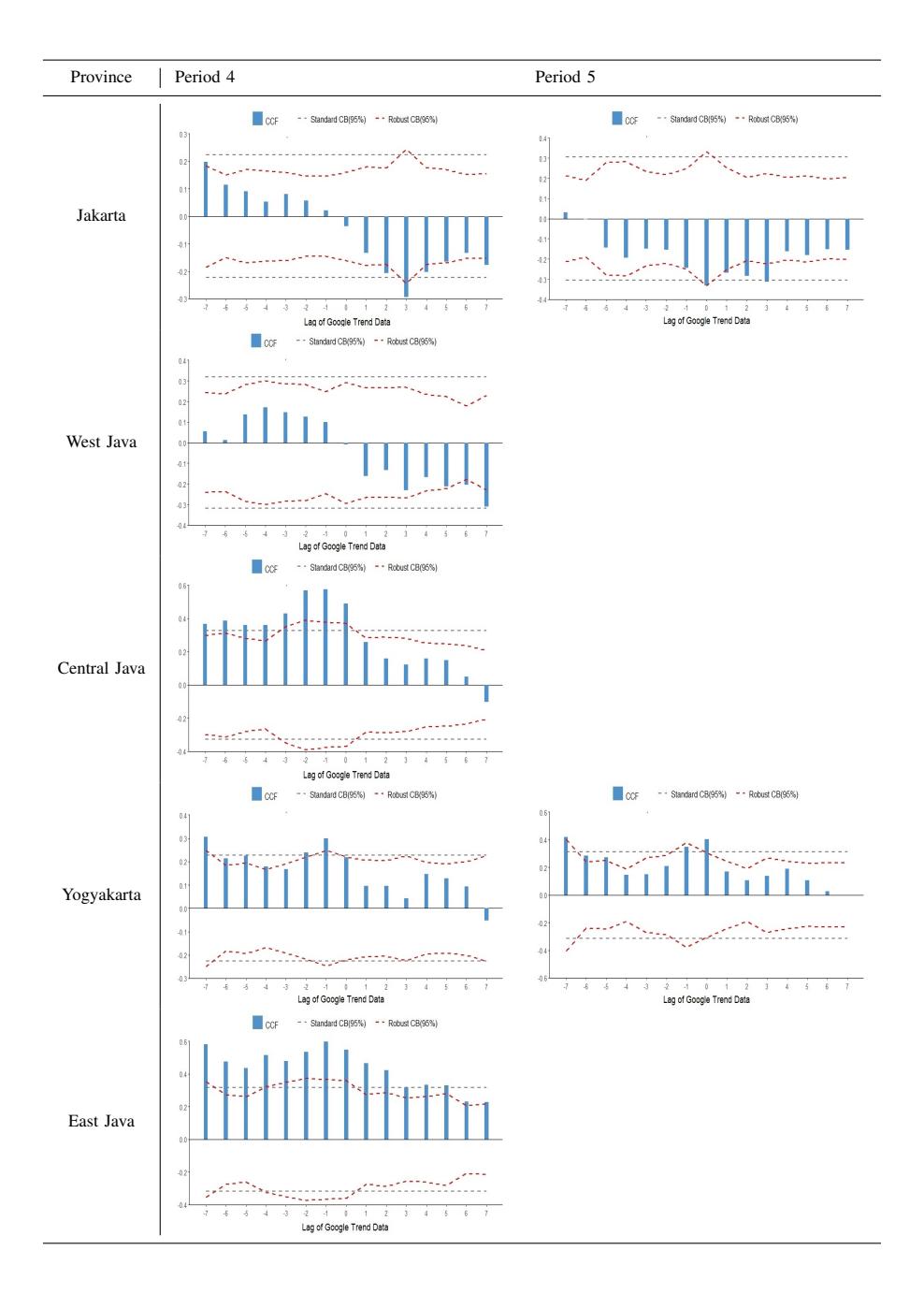
Table 3: Frequency of cumulative COVID-19 case in the provinces of Java. The cumulative data of COVID-19 cases was from the date of the first confirmed COVID-19 case in the respective province until February 14, 2021.
| Lag | Predictor | Banten | Jakarta | West Java | Central Java | Yogyakarta | East Java |
|---|---|---|---|---|---|---|---|
| GT data | 0.9316 (NR) | 0.4224 (NR) | 0.9262 (NR) | 0.3866 (NR) | 0.4979 (NR) | 0.9865 (NR) | |
| New COVID-19 Cases | 0.9877 (NR) | 0.2960 (NR) | 0.1221 (NR) | 0.0301*** (R) | 0.2658 (NR) | 0.6894 (NR) | |
| First Difference of GT index | 0.3520 (NR) | 0.0897* (R) | 0.4267 (NR) | 0.1846 (NR) | 0.9439 (NR) | 0.2769 (NR) | |
| First Difference of new COVID-19 | 0.1402 (NR) | 0.5375 (NR) | 0.2786 (NR) | 0.6731 (NR) | 0.4221 (NR) | 0.2784 (NR) | |
| 1 | Second Difference of GT index | 0.1834 (NR) | 0.0955*(R) | 0.5890 (NR) | 0.3928 (NR) | 0.6601 (NR) | 0.3074 (NR) |
| Second Difference of New COVID-19 | 0.0820*(R) | 0.2148 (NR) | 0.4566 (NR) | 0.8768 (NR) | 0.6503 (NR) | 0.0823* (R) | |
| log return google | 0.3450 (NR) | 0.01953** (R) | 0.0358* (R) | 0.0827* (R) | 0.3879 (NR) | 0.2609 (NR) | |
| log return covid | 0.06529* (R) | 0.2640 (NR) | 0.9487 (NR) | 0.5068 (NR) | 0.0828* (R) | 0.4997 (NR) | |
| GT data | 0.6141 (NR) | 0.1553 (NR) | 0.6394 (NR) | 0.2936 (NR) | 0.8742 (NR) | 0.5400 (NR) | |
| New COVID-19 Cases | 0.2872 (NR) | 0.6282 (NR) | 0.2882 (NR) | 0.1867 (NR) | 0.4834 (NR) | 0.5943 (NR) | |
| First Difference of GT index | 0.7537 (NR) | 0.2570 (NR) | 0.3516 (NR) | 0.2046 (NR) | 0.8769 (NR) | 0.5341 (NR) | |
| 2 | First Difference of New COVID-19 cases | 0.4254 (NR) | 0.7434 (NR) | 0.4892 (NR) | 0.3941 (NR) | 0.4998 (NR) | 0.5466 (NR) |
| Second Difference of GT index | 0.8209 (NR) | 0.4453 (NR) | 0.4406 (NR) | 0.1972 (NR) | 0.9415 (NR) | 0.4743 (NR) | |
| Second Difference of New COVID-19 | 0.2002 (NR) | 0.0636* (R) | 0.6578 (NR) | 0.6671 (NR) | 0.5032 (NR) | 0.3559 (NR) | |
| log return google | 0.8162 (NR) | 0.362 (NR) | 0.0750* (R) | 0.1457 (NR) | 0.8973 (NR) | 0.6205 (NR) | |
| log return covid | 0.2122 (NR) | 0.6282 (NR) | 0.2025 (NR) | 0.8630 (NR) | 0.2849 (NR) | 0.5911 (NR) | |
| GT data | 0.8510 (NR) | 0.2516 (NR) | 0.5982 (NR) | 0.2625 (NR) | 0.8941 (NR) | 0.6980 (NR) | |
| New COVID-19 Cases | 0.5531 (NR) | 0.5521 (NR) | 0.4954 (NR) | 0.3190 (NR) | 0.5229 (NR) | 0.7408 (NR) | |
| First difference of GT index | 0.8248 (NR) | 0.03323** (R) | 0.6400 (NR) | 0.5287 (NR) | 0.8360 (NR) | 0.7062 (NR) | |
| First difference of New COVID-19 | 0.2170 (NR) | 0.0004*** (R) | 0.2410 (NR) | 0.3819 (NR) | 0.5620 (NR) | 0.6054 (NR) | |
| 3 | Second Differences of GT index | 0.7965 (NR) | 0.0856* (R) | 0.5827 (NR) | 0.2025 (NR) | 0.9057 (NR) | 0.7467 (NR) |
| Second Differences of New COVID-19 | 0.3017 (NR) | 0.0069*** (R) | 0.4950 (NR) | 0.2211 (NR) | 0.6480 (NR) | 0.6076 (NR) | |
| log return google | 0.8028 (NR) | 0.09034* (R) | 0.0822* (R) | 0.2147 (NR) | 0.9680 (NR) | 0.7028 (NR) | |
| log return covid | 0.1526 (NR) | 0.1248 (NR) | 0.3048 (NR) | 0.6088 (NR) | 0.3350 (NR) | 0.7099 (NR) | |
| GT data | 0.8626 (NR) | 0.0466** (R) | 0.7783 (NR) | 0.6173 (NR) | 0.9134 (NR) | 0.4417 (NR) | |
| New COVID-19 Cases | 0.3982 (NR) | 0.0023*** (R) | 0.3835 (NR) | 0.4038 (NR) | 0.6501 (NR) | 0.7849 (NR) | |
| First Difference of GT index | 0.8233 (NR) | 0.2174 (NR) | 0.7307 (NR) | 0.6681 (NR) | 0.8653 (NR) | 0.5087 (NR) | |
| First Difference of New COVID-19 cases | 0.3533 (NR) | 0.0008*** (R) | 0.3799 (NR) | 0.5307 (NR) | 0.7135 (NR) | 0.7966 (NR) | |
| 4 | Second Difference of GT index | 0.8815 (NR) | 0.2378 (NR) | 0.8154 (NR) | 0.4959 (NR) | 0.7939 (NR) | 0.3066 (NR) |
| Second Difference of New COVID-19 | 0.4252 (NR) | 0.0121** (R) | 0.1931 (NR) | 0.1478 (NR) | 0.6478 (NR) | 0.7261 (NR) | |
| log return google | 0.8496 (NR) | 0.1927 (NR) | 0.1798 (NR) | 0.3905 (NR) | 0.9815 (NR) | 0.5438 (NR) | |
| log return google | 0.1456 (NR) | 0.2906 (NR) | 0.2902 (NR) | 0.5573 (NR) | 0.4363 (NR) | 0.8594 (NR) | |
| GT data | 0.8438 (NR) | 0.1597 (NR) | 0.8338 (NR) | 0.7705 (NR) | 0.9375 (NR) | 0.5260 (NR) | |
| New COVID-19 Cases | 0.5490 (NR) | 0.0038*** (R) | 0.5557 (NR) | 0.5192 (NR) | 0.7936 (NR) | 0.8946 (NR) | |
| First Difference of GT index | 0.7921 (NR) | 0.2379 (NR) | 0.2712 (NR) | 0.7565 (NR) | 0.8733 (NR) | 0.6132 (NR) | |
| First Difference of New COVID-19 cases | 0.5590 (NR) | 0.0006*** (R) | 0.5888 (NR) | 0.4348 (NR) | 0.8690 (NR) | 0.8363 (NR) | |
| Second Difference of GT index | 0.9525 (NR) | 0.9525 (NR) | 0.1938 (NR) | 0.8594 (NR) | 0.9250 (NR) | 0.4786 (NR) | |
| Second Difference of New COVID-19 | 0.4279 (NR) | 0.0003*** (R) | 0.1178 (NR) | 0.2773 (NR) | 0.7560 (NR) | 0.9630 (NR) | |
| log return google | 0.7807 (NR) | 0.1654 (NR) | 0.2669 (NR) | 0.5042 (NR) | 0.9965 (NR) | 0.6599 (NR) | |
| log return google | 0.4436 (NR) | 0.1447 (NR) | 0.4963 (NR) | 0.7041 (NR) | 0.4362 (NR) | 0.9026 (NR) | |
| GT data | 0.8155 (NR) | 0.1889(NR) | 0.3706 (NR) | 0.8494 (NR) | 0.9340 (NR) | 0.5890 (NR) | |
| New COVID-19 Cases | 0.7123 (NR) | 0.0027*** (R) | 0.6602 (NR) | 0.0939* (R) | 0.8985 (NR) | 0.9093 (NR) | |
| First Difference of GT index | 0.7846 (NR) | 0.5442 (NR) | 0.3879 (NR) | 0.8218 (NR) | 0.8791 (NR) | 0.6779 (NR) | |
| First Difference of New COVID-19 cases | 0.5675 (NR) | 0.0040*** (R) | 0.5613 (NR) | 0.3560 (NR) | 0.6357 (NR) | 0.8302 (NR) | |
| Second Difference of GT index | 0.4363 (NR) | 0.0939*(R) | 0.1168 (NR) | 0.9097 (NR) | 0.9523 (NR) | 0.7045 (NR) | |
| Second Difference of New COVID-19 | 0.4545 (NR) | 0.0001*** (R) | 0.2507 (NR) | 0.4610 (NR) | 0.6668 (NR) | 0.4909 (NR) | |
| log return google log return google | 0.6560 (NR) 0.2286 (NR) | 0.4372 (NR) 0.4421 (NR) | 0.3594 (NR) 0.5511 (NR) | 0.3982 (NR) 0.7493 (NR) | 0.9990 (NR) 0.2654 (NR) | 0.7921 (NR) 0.8683 (NR) | |
| 7 | |||||||
| GT data | 0.7995 (NR) | 0.2499 (NR) | 0.4288 (NR) | 0.9008 (NR) | 0.9332 (NR) | 0.6583 (NR) | |
| New COVID-19 Cases | 0.6594 (NR) | 0.0115*** (R) | 0.4723 (NR) | 0.3218 (NR) | 0.6715 (NR) | 0.9011 (NR) | |
| First Difference of GT index | 0.6602 (NR) | 0.6099 (NR) | 0.3562 (NR) | 0.8565 (NR) | 0.9469 (NR) | 0.8837 (NR) | |
| First Difference of New COVID-19 cases | 0.6793 (NR) | 0.0019*** (R) | 0.6408 (NR) | 0.4278 (NR) | 0.7149 (NR) | 0.7298 (NR) | |
| Second Difference of GT index | 0.4365 (NR) | 0.0720* (R) | 0.2325 (NR) | 0.8652 (NR) | 0.9408 (NR) | 0.8491 (NR) | |
| Second Difference of New COVID-19 | 0.5730 (NR) | 0.0005****(R) | 0.3768 (NR) | 0.4822 (NR) | 0.6179 (NR) | 0.5007 (NR) | |
| log return google log return google | 0.6419 (NR) | 0.5553 (NR) | 0.3873 (NR) | 0.3549 (NR) | 0.9990 (NR) | 0.9463 (NR) 0.9289 (NR) | |
| 0.3027 (NR) | 0.3152 (NR) | 0.7068 (NR) | 0.8446 (NR) | 0.3112 (NR) |
4.3. Causality Relationship
Table 3 shows the result of Granger Causality of each province in Indonesia from lag 1 until lag 7. Instead of Granger Causality between the original data of Covid-19 and GT data, we also conduct the result for the rate of changes in GT data and COVID-19 data also for Acceleration of the data. Since the for Granger Causality, the assumption of stationery of time series data must be full-filled, the stationery of the data is evaluated first with ADF test using R package tseries. Then, the Granger causality is performed for each pair of time series, one as predictor and the other as response. In Table 3, the left column after lag column shows the predictor of Granger Causality test. For example, if the predictor in Table 3 shows Google Trend (GT) data, then the response is New Covid-19. Further in the next row, the role is reversed, the New Covid-19 data acts as predictor and GT data acts as response. Hence, the Granger Causality is applied for 4 pairs data in total for every lag for each province with eight tests predictor-response test. The four pairs data are Google Trend data-New Covid-19 Cases, The Changes of GT index-Rate of New Covid-19 Cases, Acceleration of Gt index (second difference of GT index)-Second difference of Covid-19 cases, and logarithmic difference of GT index-logarithmic difference of Covid-19 cases.
The significant result of Granger causality relation is given with bolt result in Table 3. Here, we found that for some lags, the pairs of data have two directions cause-effect relations, but in some other lags only have one direction cause-effect relations. For example, in lag 2 for Capital Region of Jakarta, the Granger causality found only from the second difference (acceleration) of new Covid-19 cases to the second difference of GT index. But, in lag 3, it was found there are two direction cause-effect relation between these pairs data of second difference (acceleration) of new Covid-19 cases and the second difference of GT index.
The use of GT data as predictor (cause) only located in some lags in three provinces of six province. For Capital Region of Jakarta, the result shows that the role of GT data as predictor (causes) for Covid-19 cases are in lag 1,3,4,6, and 7. The interesting fact here is that only in lag 4, the original GT data can be used to predict the the occurrence of Covid-19 in future. The rest (in lag 1,2,4, and 7), the cause variables are first difference, second difference, or logarithmic difference of GT data. The role GT trend data as predictors are given in lag one until one lag 3 for West java province with the data used is logarithmic difference of GT data, instead of the original data. It show that the logarithmic difference of Google Trend data can be utilized to forecast the future behaviour of Covid-19 outbreak. For Central Java, the behaviour of logarithmic difference that is employed as predictor in Granger causality relation only occurs in lag 1. However, for the rest of three provinces, i.e. Banten, Yogyakarta, and East Java, the Granger causality take place when the Covid-19 cases data behave as the predictor. It appears, it is related as in the previous section in Table 1, the most cases of COVID-19 occurs in Jakarta, West Java, and Central Java, in this case, the GT data can be used to give the information of COVID-19 incidence. However, for Banten, Yogyakarta, and East Java, the causality can be found only at lag-1 with Covid-19 as the predictors.
5. CONCLUSION
Infodemiology analysis have given an idea in controlling and monitoring the outbreak over time and in analyzing the public's awareness and response to the outbreak of the Covid-19. In this article, we provide an insight of using information seeking patterns as an indicator to inform public health or government during pandemics such as Covid-19. One of the most infodemiology used by populations is Google. By analysing Google Trend data using specific keywords related to Covid-19, the seeking pattern over time per location can be assessed. The increased tracking for information related to COVID-19 from information search portals during the pandemic can emphasise the pandemic situation in an area where people are trying to get as much true information about the disease as possible. In another way, the public's lack of interest in seeking information about Covid-19 during a pandemic can also serve as a reminder to the government and policymakers regarding public awareness of the pandemic or stating that the situation of the spread of the disease has indeed improved.
Google Trend data extend a robust quantitative analysis to predict and observe the behaviour of Covid-19 outbreak. In this study, the analysis was applied for cases in Java island of Indonesia, with total six province level. Fist, the analysis was carried out by determining the lag-correlaiton between time series data, with lag range for -7 until 7. For each province, statistically significant lag correlations were observed which in line with previous studies that discuss the linear relationship between Covid-19 and Google Trends data. From
Table 2, the result can be explained that some periods of time, the correlation between Google Trend data and Covid-19 appear signifcantly, but not quite strong. It shows that all the correlations are below 0.6.
The second method used to approach the causal relation is Granger Causality method. For this method, the result show that at some point, in Special Region of Jakarta, West Java, and Central Java, the Google Trend data can be utilized to predict or monitor the future behaviour of Covid-19 cases. Nevertheless, the causal relation does not happen in original data most of the result. It emerged in logarithmic difference data most of the result.
This study has limitations. First, data provided for analysis is extracted only from search engine are considered. Although the information of Covid-19 may come not only from Google Search engine. Second, The Granger Causality for cross order data is not performed. For example, the Goggle trend data acts as predictor and the First Difference of Covid-19 data is as the response. Hence, any conclusions drawn from this study refer to each case individually. In spite of the limitation in this study, the use of seeking patterns metrics for monitoring and informing the outbreak of the disease has obtained extensive attention for both government and public.
ACKNOWLEDGEMENT
Part of the research is funded by ITB Research Grant 2021.