

1. INTRODUCTION
Coronavirus Disease 2019 (COVID-19) is a infectious disease for humans caused by SARS-CoV-2 [3], [24], [35]. COVID-19 affects the human respiratory system which can cause acute pneumonia [37]. COVID-19 patients generally have initial symptoms such as fever, dry cough, and fatigue [4]. The spread of COVID-19 virus through the virus in patient droplets inhaled by humans either directly or indirectly [3]. Indirect spread can be through mediums that are commonly touched by humans, such as table, office tools, and so on. The patients with strong immune systems cause them to have no symptoms (they are called asymptomatic infected) [16], [27], [36]. Therefore, COVID-19 is of global concern because patients are difficult to detect and spread quickly.
The first case of COVID-19 was confirmed in Wuhan, China, in December 2019 [37]. At first, COVID-19 was considered a common and harmless disease such as influenza. Over time, COVID-19 spread rapidly so that the World Health Organization (WHO) declared COVID-19 as world pandemic on March 11, 2020 [9]. The impact of COVID-19 pandemic is not only on human health, but indirectly it has also reduced the quality and quantity of economic sectors, social, and educational in all countries. Therefore, it is necessary to have policies from government to improve the sectors affected by this world pandemic.
The prevention and mitigation to reduce COVID-19 cases is carried out by implementing health protocols, such as wearing masks, reducing contact, wash hands routinely, and social distancing as recommended by WHO [26], [27]. In addition, other mitigation policies have also been implemented such as lockdown, quarantine especially for COVID-19 patients, mobility restrictions, maximum member capacity for an event, and so on [37]. Some of these policies are implemented by adjusting the real conditions of the disease transmission. It is important to understand the mechanism of COVID-19 spread.
*Corresponding author
Mathematical modeling is an approach to understanding the dynamics of COVID-19 spread. The model can be a phenomenological model or a mechanistic compartment model. The paper [41] conducted an analysis of growth curve of COVID-19 cases using phenomenological model including the classical logistic growth model, generalized logistic model and generalized Richard model. The phenomenological model can provide an approximation of the growth curve of COVID-19 cases to real data, both daily data and cumulative data [13], [14], [32]. On the other hand, the phenomenological model cannot provide a mechanism of COVID-19 transmission. The mechanism of COVID-19 transmission including the measurement of intervention policies can be described by compartment models [14]. Many compartment models of COVID-19 spread have been developed, such as SIR (susceptible-infected-recovered), SEIR (susceptible-exposed-infected-recovered), and other development [39], [12], [24], [40], [43], [36], [35]. In particular, Soewono [39] has appied the SEIR model to fit the early period of COVID-19 cases in Wuhan, Diamond Princess, and Jakarta-cluster.
One of policies implemented for patients is self-quarantine. In [44], Zhang et al. constructing the susceptibleexposed-infected-quarantined-recovered (SEIQR) model because the infected individuals are required by government to either self-quarantine or hospital quarantine. The quarantined individuals cannot infect others due to loss of contact with susceptible individuals [9]. The existence of a quarantined subpopulation is expected to reduce the spread of COVID-19.
Other policies implemented for uninfected individuals (such as susceptible individuals) are by applying health protocols and vaccination [18], [9]. The group of individuals who adhere to health protocols such as wearing masks and social distancing will get protection due to loss of contact with other individuals. In [27], Lopez & Rodo constructed the susceptible-exposed-infected-quarantined-recovered-death-protected ´ (SEIQRDP) model by considering the existence of protected individuals. The protected individuals who neglect health protocols will become susceptible again and they can be infected by COVID-19 viruses. In other words, there is no guarantee that a protected individual will be completely spared from COVID-19. The one can reduce the risk of death due to COVID-19 is vaccination program that prioritizes uninfected individuals (susceptible or protected individuals). In [19], Ghostine et al. constructing the susceptible-exposedinfected-quarantined-recovered-death-vaccinated (SEIQRDV) model by considering the vaccine efficacy. In vaccination program, vaccine efficacy becomes a benchmark for community as a determination to follow vaccination or not [18]. Several types of COVID-19 vaccines such as BioNTech, Moderna, Sinovac, and BNT162b2 mRNA have efficacy above 90% [23], [34]. The vaccine efficacy p < 100% causes vaccinated individuals are still possible to be infected by viruses. Since the protected individuals do not guarantee to avoid COVID-19 infection [27], the protected individuals who are vaccinated may also be infected by viruses.
COVID-19 patients who have high immunity may become an asymptomatic infected. This individual group differs from exposed individuals who are developing the virus but are not infectious [16], [27]. Megasari et al. [29] have reported asymptomatic infections in East Java, Indonesia have spread which is characterized by a high prevalence of infection. Markets and crowded places have a high risk of COVID-19 transmission by asymptomatic infection because their status is not detected. To control the presence of asymptomatic infections, rapid testing for asymptomatic and symptomatic individuals can be a strategy to reduce the basic reproduction number [6]. Hence, a mathematical model which includes the asymptomatic infected is needed. In [37], Riyapan et al. constructed the susceptible-exposed-symptomatic infected-asymptomatic infected-quarantined-recovered-death (SEIAQRD) model by considering asymptomatic infections. After virus incubation period, exposed individuals become either symptomatic or asymptomatic infected. The transmission rates of both are different. Furthermore, in [5], Adila stated that the transmission rate of asymptomatic infection was lower than symptomatic infection due to the transmission through droplets was lower.
The various characteristics of COVID-19 disease and the policies implemented are important to consider in the mathematical model. In this work, we propose the COVID-19 model by considering asymptomatic infections and the policies such as quarantine, implementing health protocols, and vaccination. First, in Section 2, we construct the susceptible-exposed-symptomatic infected-asymptomatic infected-recovered-deathprotected-quarantined-vaccination (SEIARDPQV) model. Several assumptions about vaccine efficacy in [18] are considered in the model. The first assumption is that some of vaccinated subpopulation has successfully acquired maximum immunity which is assumed to be recovered group [38]. The second assumption is that the proportion of vaccine inefficacy (failure of efficacy) from vaccinated subpopulation can be infected by COVID-19 virus. In Section 3–6, we study the dynamics of proposed model containing basic properties (non-negativity and boundedness of solutions), equilibrium points, basic reproduction number, and stability of equilibrium points, both locally and globally. In Section 7, we showed a numerical simulation using fourth
order Runge-Kutta. Finally, we conclude in Section 8.
2. MODEL FORMULATION
The model of COVID-19 transmission in this work describes the interaction between nine subpopulations, that is, S(t), E(t), I(t), A(t), R(t), D(t), P(t), Q(t), and V (t), which represent the subpopulations size of susceptible, exposed, symptomatic infected, asymptomatic infected, recovered, death due to COVID-19, protected, quarantined, and vaccinated individuals, respectively. The model assumes that susceptible individual (S(t)) may become exposed if there is a contact between susceptible individual with infected individual. Protected subpopulation (P(t)) is susceptible individuals who carry out health protocols such as wearing masks, maintaining cleanliness, social distancing, and restricting mobility. Hence, the protected subpopulation avoids contact with infected individuals. However, the protected individuals may lose their patience and become careless in implementing health protocols, and thus these individuals become susceptible again [27]. We also assumed that there are susceptible individuals who undergo a vaccination program so that they move into the vaccinated subpopulation (V (t)), where the proportion of vaccine efficacy p was successful in gaining immunity during period of a clinical experiment.
The interactions between nine subpopulations of the proposed model are shown by compartment diagram in Figure 1. The proposed model is expressed in a first-order ordinary differential equations system (1),
\[\frac{dS(t)}{dt} = \Lambda + \eta_2 P(t) - S(t) \left(\beta I(t) + \beta_a A(t)\right) - (\eta + \sigma + \mu) S(t),\] \[\frac{dE(t)}{dt} = S(t) \left(\beta I(t) + \beta_a A(t)\right) + V(t) \left(\delta I(t) + \delta_a A(t)\right) - (\alpha + \mu) E(t),\] \[\frac{dI(t)}{dt} = \theta \alpha E(t) - (\gamma + \gamma_4 + \mu) I(t),\] \[\frac{dA(t)}{dt} = (1 - \theta) \alpha E(t) - (\gamma_a + \gamma_5 + \mu) A(t),\] \[\frac{dR(t)}{dt} = \nu Q(t) + q V(t) + b \gamma I(t) + \gamma_a A(t) - \mu R(t),\] \[\frac{dD(t)}{dt} = \nu_2 Q(t) + (1 - b) \gamma I(t),\] \[\frac{dP(t)}{dt} = \eta S(t) - (\eta_2 + \sigma_1 + \mu) P(t),\] \[\frac{dQ(t)}{dt} = \gamma_4 I(t) + \gamma_5 A(t) - (\nu + \nu_2 + \mu) Q(t),\] \[\frac{dV(t)}{dt} = \sigma S(t) + \sigma_1 P(t) - V(t) \left(\delta I(t) + \delta_a A(t)\right) - (q + \mu) V(t),\]
with non-negative initial values S(0) = S0, E(0) = E0, I(0) = I0, A(0) = A0, R(0) = R0, D(0) = D0, P(0) = P0, Q(0) = Q0, V (0) = V0. The definition of parameters in model (1) could be seen in Table 1. To simplify the model (1), we introduce new symbols ξ1 = η + σ + µ, ξ2 = α + µ, ξ3 = γ + γ4 + µ, ξ4 = γa + γ5 + µ, ξ5 = η2 + σ1 + µ, ξ6 = ν + ν2 + µ, and ξ7 = q + µ. Since the first four equations and the last three equations of Model (1) do not depend on R(t) and D(t), we reduce the nine-dimensional model to a seven-dimensional model expressed in System (2).
\[\frac{dS(t)}{dt} = \Lambda + \eta_2 P(t) - S(t) \left(\beta I(t) + \beta_a A(t)\right) - \xi_1 S(t),\] \[\frac{dE(t)}{dt} = S(t) \left(\beta I(t) + \beta_a A(t)\right) + V(t) \left(\delta I(t) + \delta_a A(t)\right) - \xi_2 E(t),\] \[\frac{dI(t)}{dt} = \theta \alpha E(t) - \xi_3 I(t),\] \[\frac{dA(t)}{dt} = (1 - \theta) \alpha E(t) - \xi_4 A(t),\] \[\frac{dP(t)}{dt} = \eta S(t) - \xi_5 P(t),\] \[\frac{dQ(t)}{dt} = \gamma_4 I(t) + \gamma_5 A(t) - \xi_6 Q(t),\] \[\frac{dV(t)}{dt} = \sigma S(t) + \sigma_1 P(t) - V(t) \left(\delta I(t) + \delta_a A(t)\right) - \xi_7 V(t).\] (2)
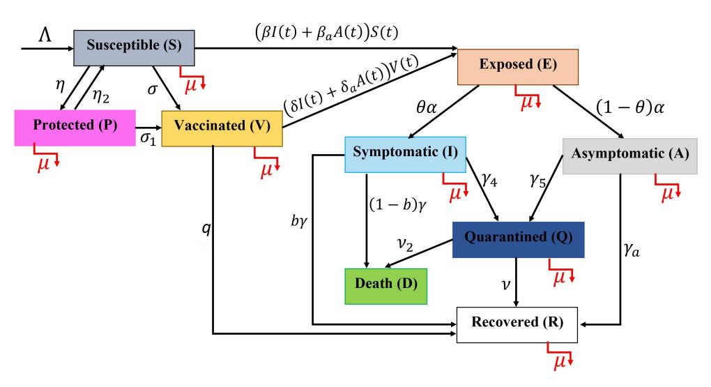
Figure 1: The compartment diagram of the proposed COVID-19 epidemic model.
3. NON-NEGATIVITY AND BOUNDEDNESS OF SOLUTIONS
Since Model (2) describes the interaction of human subpopulations, the solutions of the system must be nonnegative and ultimately bounded. The following theorem has guaranteed the non-negativity and boundedness of solutions of Model (2).
Theorem 3.1. All solutions of the reduced COVID-19 Model (2) subject to non-negative initial values are non-negative and ultimately bounded.
Proof: We first prove that S(t) and P(t) are non-negative. Assume the contrary; then let t1 and t2 be the first time such that they are equal to zero at t1 and t2, respectively. From first and fifth equations of Model (2), we get
Table 1: The definition of parameters in Model (2).
| Parameter | Definition | |
|---|---|---|
| Λ | Recruitment rate of \(S(t)\) | |
| \(\mu\) | Natural death rate | |
| \(\eta\) | Protection rate | |
| \(\eta_2\) | Rate of carelessness in protection | |
| \(\sigma\) | Vaccination rate of \(S(t)\) | |
| \(\sigma_1\) | Vaccination rate of \(P(t)\) | |
| p | Vaccine efficacy | |
| q | p/(Average time that V(t) need to obtain immunity) | |
| \(\begin{array}{c} q \ \beta \ \beta_a \end{array}\) | Transmission rate in \(S(t)\) from symptomatic infection | |
| \(\beta_a\) | Transmission rate in \(S(t)\) from asymptomatic infection | |
| \[\delta = (1 - p)\beta\] | Transmission rate in \(V(t)\) from symptomatic infection | |
| \[\delta_a = (1 - p)\beta_a\] | Transmission rate in \(V(t)\) from asymptomatic infection | |
| \(\alpha\) | 1/(Average incubation period) | |
| \(\theta\) | Symptomatic proportion | |
| \(\gamma\) | Disease-free rate of \(I(t)\) | |
| b | Recovery proportion | |
| \(\gamma_4\) | Quarantine rate of \(I(t)\) | |
| \(\gamma_a\) | Recovery rate of \(A(t)\) | |
| \(\gamma_5\) | Quarantine rate of \(A(t)\) | |
| \(\nu\) | Recovery rate of \(Q(t)\) | |
| \(\nu_2\) | COVID-19 death rate of \(Q(t)\) | |
\[\frac{dS(t)}{dt}\Big|_{t=t_1} = \Lambda + \eta_2 P(t_1),\] \[\frac{dP(t)}{dt}\Big|_{t=t_2} = \eta S(t_2).\] (3)
Since the right-hand side of equations (3) depends on \(t_1\) and \(t_2\), we separate this proof into two cases. If \(t_1 \le t_2\), then \(P(t_1) \ge 0\). We have
\[\frac{dS(t)}{dt}\Big|_{t=t_1} = \Lambda + \eta_2 P(t_1) > 0.\]
This means that S(t)>0 on \((t_1,t_1+\varepsilon_1)\) for arbitrary small positive constant \(\varepsilon_1\). This leads to a contradiction. As a result, \(S(t)\geq 0\) for all \(t\geq 0\). Consequently, \(\frac{dP(t)}{dt}|_{t=t_2}=\eta S(t_2)\geq 0\). Similarly, \(P(t)\geq 0\) on \((t_2,t_2+\varepsilon_2)\) for arbitrary small positive constant \(\varepsilon_2\). This leads to a contradiction. As a result, \(P(t)\geq 0\) for all \(t\geq 0\). If \(t_1>t_2\), then \(S(t_2)>0\). We have
\[\left. \frac{dP(t)}{dt} \right|_{t=t_2} = \eta S(t_2) > 0.\]
This means that P(t)>0 on \((t_2,t_2+\varepsilon_2)\) for arbitrary small positive constant \(\varepsilon_2\). This leads to a contradiction. As a result, \(P(t)\geq\) for all \(t\geq 0\). Consequently, \(\frac{dS(t)}{dt}|_{t=t_1}=\Lambda+P(t_1)>0\). Similarly, S(t)>0 on \((t_1,t_1+\varepsilon_1)\) for arbitrary small positive constant \(\varepsilon_1\). This leads to a contradiction. As a result, \(S(t)\geq 0\) for all t>0.
The non-negativity of E(t), I(t), A(t), Q(t), V(t) can also been shown in similar way. Therefore, all solutions of Model (2) are non-negative.
We next let N(t) = S(t) + E(t) + I(t) + A(t) + P(t) + Q(t) + V(t). Based on Model (2), we have
\[\frac{dN(t)}{dt} = \Lambda - \mu N(t) - pV(t) - \gamma I(t) - (\nu + \nu_2) Q(t) - \gamma_a A(t) \le \Lambda - \mu N(t).\]
It is easy to show that N(t) satisfies
\[N(t) \le \frac{\Lambda}{\mu} + \left(N(0) - \frac{\Lambda}{\mu}\right) \exp(-\mu t),\] and thus \(\lim_{t\to +\infty} N(t) \leq \frac{\Lambda}{\mu}\). The feasible region of Model (2) is
\[\Omega = \left\{ (S, E, I, A, P, Q, V) \in \mathbb{R}^7_+ \cup \{\vec{0}\} \middle| S + E + I + A + P + Q + V \le \frac{\Lambda}{\mu} \right\}.\]
Therefore, all solutions of Model (2) are ultimately bounded.
4. EQULIBRIUM POINTS AND BASIC REPRODUCTION NUMBER
We first let \(\omega = \frac{\beta\theta\alpha}{\xi_3} + \frac{\beta_a(1-\theta)\alpha}{\xi_4}\), \(\Psi_1 = \frac{\xi_7}{(1-p)}\), \(\Psi_2 = \frac{\mu\eta}{\xi_5} + \mu\), and X(t) = (S(t), E(t), I(t), A(t), P(t), Q(t), V(t)). By setting the right-hand side of equations in Model (2) to be zero, we get the solutions as equilibrium points. We see the second equation of Model (2):
\[S(t) \left( \frac{\beta \theta \alpha}{\xi_3} + \frac{\beta_a (1 - \theta) \alpha}{\xi_4} \right) E(t) + V(t) \left( \frac{\delta \theta \alpha}{\xi_3} + \frac{\delta_a (1 - \theta) \alpha}{\xi_4} \right) E(t) - \xi_2 E(t) = 0.\]
It is clear that either E(t)=0 or \(S(t)\left(\frac{\beta\theta\alpha}{\xi_3}+\frac{\beta_a(1-\theta)\alpha}{\xi_4}\right)+V(t)\left(\frac{\delta\theta\alpha}{\xi_3}+\frac{\delta_a(1-\theta)\alpha}{\xi_4}\right)=\xi_2\), from which we obtain two equilibrium points of Model (2), that is, disease-free equilibrium point \(\chi^{DFE}\) and endemic equilibrium point \(\chi^*\). The disease-free equilibrium point is \(\chi^{DFE}(S^{DFE},0,0,0,P^{DFE},0,V^{DFE})\) with
\[S^{DFE} = \frac{\Lambda \xi_5}{\xi_1 \xi_5 - \eta_2 \eta}, \quad P^{DFE} = \frac{\Lambda \eta}{\xi_1 \xi_5 - \eta_2 \eta}, \quad V^{DFE} = \frac{\Lambda (\sigma \xi_5 + \sigma_1 \eta)}{\xi_7 (\xi_1 \xi_5 - \eta_2 \eta)},\] which is always exists.
We next determine the basic reproduction number \((\mathcal{R}_0)\) of Model (2). First, we define Y(t) = (E(t), I(t), A(t), Q(t)), which is the vector of infected compartment. The expression \(\frac{d}{dt}Y(t)\) can be represented by \(\frac{d}{dt}Y(t) = \mathcal{F} - \mathcal{M}\) where
\[\mathcal{F} = \begin{pmatrix} S(t) \left( \beta I(t) + \beta_a A(t) \right) + V(t) \left( \delta I(t) + \delta_a A(t) \right) \\ 0 \\ 0 \\ 0 \end{pmatrix},\] and
\[\mathcal{M} = \begin{pmatrix} \xi_2 E(t) \\ -\theta \alpha E(t) + \xi_3 I(t) \\ -(1-\theta)\alpha E(t) + \xi_4 A(t) \\ -\gamma_4 I(t) - \gamma_5 A(t) + \xi_6 Q(t) \end{pmatrix}.\]
The Jacobian matrices of \(\mathcal{F}\) and \(\mathcal{M}\) at \(\chi^{DFE}\) are respectively
\[\text{[rumus tidak dapat ditampilkan dengan baik — lihat PDF asli]}\] and
\[M = \begin{pmatrix} \xi_2 & 0 & 0 & 0 \\ -\theta \alpha & \xi_3 & 0 & 0 \\ -(1-\theta)\alpha & 0 & \xi_4 & 0 \\ 0 & -\gamma_4 & -\gamma_5 & \xi_6 \end{pmatrix}.\]
Then the next generation matrix is
\[\text{[rumus tidak dapat ditampilkan dengan baik — lihat PDF asli]}\] where \(\mathcal{R}_I = \frac{\Lambda \xi_5}{\Psi_1 \xi_2 (\xi_1 \xi_5 - \eta_2 \eta)} \left( \Psi_1 + \sigma + \frac{\sigma_1 \eta}{\xi_5} \right) \left( \frac{\beta \theta \alpha}{\xi_3} \right)\) and \(\mathcal{R}_A = \frac{\Lambda \xi_5}{\Psi_1 \xi_2 (\xi_1 \xi_5 - \eta_2 \eta)} \left( \Psi_1 + \sigma + \frac{\sigma_1 \eta}{\xi_5} \right) \left( \frac{\beta a (1 - \theta) \alpha}{\xi_4} \right)\). The basic reproduction number is the radius spectral \(\rho\) of the next generation matrix, which in our case is given by
\[\begin{array}{rcl} \mathcal{R}_{0} & = & \rho(FM^{-1}) \\ & = & \mathcal{R}_{I} + \mathcal{R}_{A} \\ & = & \frac{\Lambda \xi_{5}}{\Psi_{1} \xi_{2} (\xi_{1} \xi_{5} - \eta_{2} \eta)} \left( \Psi_{1} + \sigma + \frac{\sigma_{1} \eta}{\xi_{5}} \right) \left( \frac{\beta \theta \alpha}{\xi_{3}} + \frac{\beta_{a} (1 - \theta) \alpha}{\xi_{4}} \right) \end{array}\]
We notice that the basic reproduction number has two terms which are from the symptomatic and asymptomatic infections, respectively [37].
The second equilibrium point is endemic equilibrium point \(\chi^*(S^*, E^*, I^*, A^*, P^*, Q^*, V^*)\) with
\[S^* = \frac{\Lambda}{\xi_1 - \frac{\eta_2 \eta}{\xi_5} + \omega E^*}, \quad I^* = \frac{\theta \alpha}{\xi_3} E^*, \quad A^* = \frac{(1 - \theta)\alpha}{\xi_4} E^*, \quad P^* = \frac{\eta \Lambda}{\xi_1 \xi_5 - \eta_2 \eta + \omega \xi_5 E^*},\]\[Q^* = \left(\frac{\gamma_4 \theta \alpha}{\xi_3 \xi_6} + \frac{\gamma_5 (1 - \theta)\alpha}{\xi_4 \xi_6}\right) E^*, \quad V^* = \frac{\xi_2}{(1 - p)\omega} - \frac{\Lambda}{(1 - p)\left(\xi_1 - \frac{\eta_2 \eta}{\xi_5} + \omega E^*\right)},\] where \(E^*\) satisfies the following quadratic equation:
\[A_1(E^*)^2 + A_2E^* + A_3 = 0, (4)\] with
\[\begin{split} A_1 &= \xi_2 \omega, \\ A_2 &= \Psi_1 \xi_2 - \frac{\eta_2 \eta \xi_2}{\xi_5} + \xi_1 \xi_2 - \omega \Lambda, \\ A_3 &= \frac{\xi_1 \xi_2 \Psi_1}{\omega} - \Lambda \xi_1 - \frac{\eta_2 \eta \xi_2 \Psi_1}{\xi_5 \omega} + \frac{\eta_2 \eta \Lambda}{\xi_5} - \Lambda (\Psi_1 - \Psi_2). \end{split}\]
The existence and uniqueness of endemic equilibrium point is given by following theorem.
Theorem 4.1. The endemic equilibrium point \(\chi^*\) exists and unique if \(\mathcal{R}_0 > 1\), and does not exist if \(\mathcal{R}_0 < 1\).
Proof: Suppose that \(\mathcal{D}\) represents a discriminant of Equation (4). We first proof that the endemic equilibrium point \(\chi^*\) exists and unique if \(\mathcal{R}_0 > 1\). If \(\mathcal{R}_0 > 1\), then \(\frac{\Delta \omega}{\xi_2} \left( \Psi_1 - \Psi_2 + \xi_1 - \frac{\eta_2 \eta}{\xi_5} \right) > \frac{\Psi_1(\xi_1 \xi_5 - \eta_2 \eta)}{\xi_5}\). We consider that
\[-4A_{1}A_{3} = -4\xi_{2}^{2} \left( \xi_{1}\Psi_{1} - \frac{\Lambda\xi_{1}\omega}{\xi_{2}} - \frac{\eta_{2}\eta\Psi_{1}}{\xi_{5}} + \frac{\eta_{2}\eta\omega\Lambda}{\xi_{5}\xi_{2}} - \frac{\Lambda\omega(\Psi_{1} - \Psi_{2})}{\xi_{2}} \right)\] \[= 4\xi_{2}^{2} \left( \left( \frac{\Lambda\omega(\Psi_{1} - \Psi_{2})}{\xi_{2}} + \frac{\Lambda\xi_{1}\omega}{\xi_{2}} - \frac{\eta_{2}\eta\omega\Lambda}{\xi_{5}\xi_{2}} \right) - \Psi_{1} \left( \xi_{1} - \frac{\eta_{2}\eta}{\xi_{5}} \right) \right)\] \[> 0.\]
Therefore, \(E^*=\frac{-A_2+\sqrt{\mathcal{D}}}{2A_1}>0\) if \(\mathcal{R}_0>1\), which is unique.
The positivity \(V^*>0\) is equivalent to \(\frac{\Lambda}{\xi_1-\frac{\eta_2\eta}{\xi_2}+\omega E^*}<\frac{\xi_2}{\omega}\). In other words, by substituting \(E^*\), we have to show \(\sqrt{\mathcal{D}}>\xi_2\left(\Psi_1-\xi_1+\frac{\eta_2\eta}{\xi_5}+\frac{\omega\Lambda}{\xi_2}\right)\) if \(\mathcal{R}_0>1\). We consider that
\[\mathcal{D} = \xi_{2}^{2} \left( \Psi_{1} - \frac{\eta_{2}\eta}{\xi_{5}} + \xi_{1} - \frac{\omega\Lambda}{\xi_{2}} \right)^{2}\] \[+4\xi_{2}^{2} \left( \left( \frac{\omega\Lambda(\Psi_{1} - \Psi_{2})}{\xi_{2}} + \frac{\Lambda\omega\xi_{1}}{\xi_{2}} - \frac{\eta_{2}\eta\omega\Lambda}{\xi_{5}\xi_{2}} \right) - \Psi_{1} \left( \xi_{1} - \frac{\eta_{2}\eta}{\xi_{5}} \right) \right)\] \[= \xi_{2}^{2} \left( \Psi_{1}^{2} + 2\Psi_{1} \left( \xi_{1} - \frac{\eta_{2}\eta}{\xi_{5}} - \frac{\omega\Lambda}{\xi_{2}} \right) + \left( \xi_{1} - \frac{\eta_{2}\eta}{\xi_{5}} - \frac{\omega\Lambda}{\xi_{2}} \right)^{2} \right)\] \[+4\xi_{2}^{2} \left( \left( \frac{\omega\Lambda(\Psi_{1} - \Psi_{2})}{\xi_{2}} + \frac{\Lambda\omega\xi_{1}}{\xi_{2}} - \frac{\eta_{2}\eta\omega\Lambda}{\xi_{5}\xi_{2}} \right) - \Psi_{1} \left( \xi_{1} - \frac{\eta_{2}\eta}{\xi_{5}} \right) \right)\] \[= \xi_{2}^{2} \left( \Psi_{1}^{2} - 2\Psi_{1} \left( \xi_{1} - \frac{\eta_{2}\eta}{\xi_{5}} - \frac{\omega\Lambda}{\xi_{2}} \right) + \left( \xi_{1} - \frac{\eta_{2}\eta}{\xi_{5}} - \frac{\omega\Lambda}{\xi_{2}} \right)^{2} \right)\] \[+4\xi_{2}\Lambda\omega \left( \xi_{1} - \frac{\eta_{2}\eta}{\xi_{5}} - \Psi_{2} \right)\] \[> \xi_{2}^{2} \left( \Psi_{1} - \xi_{1} + \frac{\eta_{2}\eta}{\xi_{5}} + \frac{\omega\Lambda}{\xi_{2}} \right)^{2}.\]
It is clear that \(\sqrt{\mathcal{D}} > \xi_2 \left( \Psi_1 - \xi_1 + \frac{\eta_2 \eta}{\xi_5} + \frac{\omega \Lambda}{\xi_2} \right)\). Therefore, the endemic equilibrium exists and unique if \(\mathcal{R}_0 > 1\).
We next proof that the endemic equilibrium point does not exist if \(\mathcal{R}_0 < 1\). If \(\mathcal{R}_0 < 1\), then \(\frac{\Psi_1(\xi_1\xi_5 - \eta_2\eta)}{\xi_5\omega} > \frac{\Lambda}{\xi_2} \left( \Psi_1 - \Psi_2 + \xi_1 - \frac{\eta_2\eta}{\xi_5} \right)\) and \(\xi_1 - \frac{\eta_2\eta}{\xi_5} > \frac{\omega\Lambda}{\Psi_1\xi_2} \left( (\Psi_1 - \Psi_2) + \xi_1 - \frac{\eta_2\eta}{\xi_5} \right) > \frac{\omega\Lambda}{\xi_2}\). We consider that
\[\begin{array}{lcl} \frac{A_3}{A_1} & = & \frac{\xi_1\Psi_1}{\omega^2} - \frac{\Lambda\xi_1}{\xi_2\omega} - \frac{\eta_2\eta\Psi_1}{\xi_5\omega^2} + \frac{\eta_2\eta\Lambda}{\xi_5\xi_2\omega} - \Lambda\frac{(\Psi_1-\Psi_2)}{\xi_2\omega} \\ & = & \frac{\Psi_1(\xi_1\xi_5-\eta_2\eta)}{\xi_5\omega^2} - \frac{\Lambda\xi_1}{\xi_2\omega} + \frac{\eta_2\eta\Lambda}{\xi_5\xi_2\omega} - \Lambda\frac{(\Psi_1-\Psi_2)}{\xi_2\omega} \\ & > & 0, \end{array}\] and
\[\frac{A_2}{A_1} = \frac{1}{\omega} \left( \Psi_1 + \xi_1 - \frac{\eta_2 \eta}{\xi_5} - \frac{\omega \Lambda}{\xi_2} \right)\] \[> 0.\]
This means that Equation (4) has no positive solution. Thus, Theorem 4.1 is proven.
5. LOCAL STABILITY
In this section, we investigate the local stability of equilibrium points of non-linear Model (2) with linearization around equilibrium points. In this linearization, the Jacobian matrix at equilibrium point \(\chi^k\) is given by
\[J(\chi^k) = \begin{pmatrix} J_1 & 0 & -\beta S^k & -\beta_a S^k & \eta_2 & 0 & 0 \\ \omega E^k & -\xi_2 & \beta S^k + \delta V^k & \beta_a S^k + \delta_a V^k & 0 & 0 & (1-p)\omega E^k \\ 0 & \theta \alpha & -\xi_3 & 0 & 0 & 0 & 0 \\ 0 & (1-\theta)\alpha & 0 & -\xi_4 & 0 & 0 & 0 \\ \eta & 0 & 0 & 0 & -\xi_5 & 0 & 0 \\ 0 & 0 & \gamma_4 & \gamma_5 & 0 & -\xi_6 & 0 \\ \sigma & 0 & -\delta V^k & -\delta_a V^k & \sigma_1 & 0 & J_2 \end{pmatrix},\]
with \(J_1 = -\omega E^k - \xi_1\) and \(J_2 = -(1-p)\omega E^k - \xi_7\). By evaluating the real part of all eigenvalues of the Jacobian matrix, we get the following stability conditions for the disease-free equilibrium point and the endemic equilibrium point.
Theorem 5.1. The disease-free equilibrium point \(\chi^{DFE}\) of Model (2) is locally asymptotically stable if \(\mathcal{R}_0 < 1\).
Proof: Assume that \(\mathcal{R}_0 < 1\). By evaluating \(|J(\chi^{DFE}) - \lambda I| = 0\), we have the characteristic equation of Jacobian matrix J at \(\chi^{DFE}\) as follow.
\[(-\xi_7 - \lambda)(-\xi_6 - \lambda)((-\xi_5 - \lambda)(-\xi_1 - \lambda) - \eta_2 \eta)(b_1 + b_2) = 0,\] (5)
with
\[b_1 = (-\xi_4 - \lambda) \left( (-\xi_2 - \lambda)(-\xi_3 - \lambda) - \theta \alpha (\beta S^{DFE} + \delta V^{DFE}) \right),\]
\[b_2 = (1 - \theta) \alpha (\xi_3 + \lambda) (\beta_a S^{DFE} + \delta_a V^{DFE}).\]
It is clear that the first two eigenvalues are \(\lambda_1=-\xi_6<0\) and \(\lambda_2=-\xi_7<0\). Two other eigenvalues \((\lambda_3,\lambda_4)\) are determined by \(((-\xi_5-\lambda)(-\xi_1-\lambda)-\eta_2\eta)=0\) or equivalently by \(\lambda^2+(\xi_1+\xi_5)\lambda+(\xi_1\xi_5-\eta_2\eta)=0\). Since \(-(\xi_1+\xi_5)<0\) and \(\xi_1\xi_5-\eta_2\eta>0\), the real parts of eigenvalues \(\lambda_3\) and \(\lambda_4\) are negative. The rest of eigenvalues are determined by \(b_1+b_2=0\). By recalling the equalities \(\theta\alpha(\beta S^{DFE}+\delta V^{DFE})=\xi_2\xi_3\mathcal{R}_I\) and \((1-\theta)\alpha(\beta_a S^{DFE}+\delta_a V^{DFE})=\xi_2\xi_4\mathcal{R}_A\), \(b_1+b_2=0\) can be written as
\[\lambda^3 + c_1 \lambda^2 + c_2 \lambda + c_3 = 0 \tag{6}\] where \(c_1 = (\xi_1 + \xi_2 + \xi_3)\), \(c_2 = ((1 - \mathcal{R}_I)\xi_2\xi_3 + (1 - \mathcal{R}_A)\xi_2\xi_4 + \xi_4\xi_3)\), and \(c_3 = \xi_2\xi_3\xi_4(1 - \mathcal{R}_0)\).
Based on the well-known Routh-Hurwitz Criterion, the solutions of Equation (6) have negative real parts if and only if \(c_1>0\), \(c_3>0\), and \(c_1c_2-c_3>0\). We see that \(c_1\) is always positive and if \(\mathcal{R}_0<1\), then \(c_3=\xi_2\xi_3\xi_4(1-\mathcal{R}_0)>0\). Furthermore, if \(\mathcal{R}_0<1\), then \(\mathcal{R}_I<1\) and \(\mathcal{R}_A<1\). Hence, \(c_1c_2-c_3=((1-\mathcal{R}_I)\xi_2\xi_3+(1-\mathcal{R}_A)\xi_2\xi_4)\) \((\xi_1+\xi_2+\xi_3)+\xi_1\xi_4\xi_3+\xi_3^2\xi_4+\mathcal{R}_0\xi_2\xi_3\xi_4>0\). Therefore, all solutions of the characteristic Equation (5) have negative real parts if \(\mathcal{R}_0<1\). In other words, the disease-free equilibrium point is locally asymptotically stable if \(\mathcal{R}_0<1\).
Theorem 5.2. Let the endemic equilibrium point \(\chi^*\) of Model (2) exists. The point \(\chi^*\) is locally asymptotically stable if \(\Delta_3 > 0\), and \(\Delta_5 > 0\) where \(\Delta_3\) and \(\Delta_5\) are stated in the proof.
Proof: We first assume that the endemic equilibrium \(\chi^*\) exists and use the following notations
\[\begin{array}{lll} Y_1 & = & -(\xi_2+\xi_3+\xi_4) < 0, \\ Y_2 & = & \left(\frac{\xi_2\beta\theta\alpha}{\omega} + \frac{\xi_2\beta_a(1-\theta)\alpha}{\omega} - \xi_2\xi_3 - \xi_2\xi_4 - \xi_3\xi_4\right) < 0, \\ Y_4 & = & -(\beta\theta+\beta_a(1-\theta))\alpha S^* < 0, \\ Y_5 & = & \omega\xi_3\xi_4S^* > 0, \\ Y_6 & = & -(\delta\theta+\delta_a(1-\theta))\alpha V^* < 0, \\ Y_7 & = & \omega\xi_3\xi_4(1-p)V^* > 0, \\ Y_8 & = & -(\omega E^*+\xi_1) + Y_1 < 0, \\ Y_9 & = & -(\omega E^*+\xi_1)Y_1 - Y_2 > 0, \\ Y_{10} & = & -(\omega E^*+\xi_1)Y_2 - \omega E^*Y_4 > 0, \\ Y_{11} & = & \omega E^*Y_5 > 0, \\ Y_{12} & = & \eta\left(\sigma_1Y_4 - \eta_2Y_6\right), \\ Y_{13} & = & \eta\left(\eta_2Y_7 - \sigma_1Y_5\right). \end{array}\]
By evaluating \(|J(\chi^*) - \lambda I| = 0\), the characteristic equation of the Jacobian matrix J at \(\chi^*\) can be written as
\[(-\xi_6 - \lambda) \left(\lambda^6 + W_1 \lambda^5 + W_2 \lambda^4 + W_3 \lambda^3 + W_4 \lambda^2 + W_5 \lambda + W_6\right) = 0, \tag{7}\] where
\[\begin{array}{lll} W_1 &=& \xi_5 - Y_8 + (1-p)\omega E^* + \xi_7, \\ W_2 &=& Y_9 - \xi_5 Y_8 - \eta_2 \eta + ((1-p)\omega E^* + \xi_7) \left(\xi_5 - Y_8\right), \\ W_3 &=& \xi_5 Y_9 + Y_{10} + \eta_2 \eta Y_1 - (1-p)\omega E^* Y_6 + ((1-p)\omega E^* + \xi_7) \left(Y_9 - \xi_5 Y_8 - \eta_2 \eta\right), \\ W_4 &=& \xi_5 Y_{10} + Y_{11} + \eta_2 \eta Y_2 + ((1-p)\omega E^* + \xi_7) \left(\xi_5 Y_9 + Y_{10} + \eta_2 \eta Y_1\right) \\ && + (1-p)\omega E^* \left(Y_7 - (\omega E^* + \xi_1)Y_6 - \sigma Y_4 - \xi_5 Y_6\right), \\ W_5 &=& \xi_5 Y_{11} + ((1-p)\omega E^* + \xi_7) \left(\xi_5 Y_{10} + Y_{11} + \eta_2 \eta Y_2\right) \\ && + (1-p)\omega E^* \left(\xi_5 Y_7 - \xi_5 (\omega E^* + \xi_1)Y_6 - \xi_5 \sigma Y_4 + \sigma Y_5 + (\omega E^* + \xi_1)Y_7 - Y_{12}\right), \\ W_6 &=& \left((1-p)\omega E^* + \xi_7\right) \left(\xi_5 Y_{11}\right) + (1-p)\omega E^* \left(\xi_5 \sigma Y_5 + (\omega E^* + \xi_1)\xi_5 Y_7 - Y_{13}\right). \end{array}\]
From Equation (7), we get the first eigenvalue \(\lambda_1 = -\xi_6 < 0\). We next show that \(W_i > 0\) for all i = 1, 2, ..., 6.
- 1) It is clear that \(W_1 > 0\).
- Since \(-\xi_5 Y_8 > \xi_5 \xi_1 > \eta_2 \eta\), \(\xi_5 Y_9 > -\eta_2 \eta Y_1\), and \(\xi_5 Y_{10} > -\eta_2 \eta Y_2\), we have \(W_2 > 0\), \(W_3 > 0\), and 2) \(W_4 > 0\).
- Since \(\xi_5 Y_{10} > -\eta_2 \eta Y_2\) and \(-\xi_5 (\omega E^* + \xi_1) Y_6 > \eta_2 \eta Y_6 > Y_{12}\), we have \(W_5 > 0\). Since \((\omega E^* + \xi_1) \xi_5 Y_7 > \eta_2 \eta Y_7 > Y_{13}\), we have \(W_6 > 0\).
Based on Lienard-Chipart Criterion in [15], all characteristics roots of Equation (7) have negative real parts if and only if the third and the fifth Routh-Hurwitz Criterion are satisfied, that are \(\Delta_3 > 0\), and \(\Delta_5 > 0\), where
\[\Delta_3 = \begin{vmatrix} W_1 & 1 & 0 \\ W_3 & W_2 & W_1 \\ W_5 & W_4 & W_3 \end{vmatrix} = W_3(W_1W_2 - W_3) - W_1(W_1W_4 - W_5) > 0,\] and
\[\Delta_{5} = \begin{vmatrix} W_{1} & 1 & 0 & 0 & 0 \\ W_{3} & W_{2} & W_{1} & 1 & 0 \\ W_{5} & W_{4} & W_{3} & W_{2} & W_{1} \\ 0 & W_{6} & W_{5} & W_{4} & W_{3} \\ 0 & 0 & 0 & W_{6} & W_{5} \end{vmatrix} = W_{5}[W_{4}\Delta_{3} - W_{2}(W_{1}(W_{2}W_{5} - W_{1}W_{6}) - W_{3}W_{5}) - W_{3}W_{5})] + W_{1}(W_{4}W_{5} - W_{3}W_{6}) - W_{5}^{2}] - W_{6}[W_{3}\Delta_{3} - W_{1}(W_{1}(W_{2}W_{5} - W_{1}W_{6}) - W_{3}W_{5})] + W_{1}(W_{1}(W_{2}W_{5} - W_{1}W_{6}) - W_{3}W_{5})] + W_{1}(W_{1}(W_{2}W_{5} - W_{1}W_{6}) - W_{3}W_{5})] + W_{2}(W_{1}(W_{2}W_{5} - W_{1}W_{6}) - W_{3}W_{5})] + W_{3}(W_{1}(W_{2}W_{5} - W_{1}W_{6}) - W_{3}W_{5})] + W_{3}(W_{1}(W_{2}W_{5} - W_{1}W_{6}) - W_{3}W_{5})] + W_{3}(W_{1}(W_{2}W_{5} - W_{1}W_{6}) - W_{3}W_{5})]\]
Therefore, the endemic equilibrium point \(\chi^*\) is locally asymptotically stable if \(\Delta_3 > 0\), and \(\Delta_5 > 0\).
6. GLOBAL STABILITY
In this section, we investigate the global stability of equilibrium points by introducing suitable Lyapunov functions. The conditions for global stability of the equilibrium point of Model (2) are given by the following theorems.
Theorem 6.1. The disease-free equilibrium point \(\chi^{DFE}(S^{DFE}, 0, 0, 0, P^{DFE}, V^{DFE})\) of Model (2) is globally asymptotically stable if \(\mathcal{R}_0 < 1\).
Proof: Assume that \(\mathcal{R}_0 < 1\) and let \(\mathcal{Z}(x) = (x - 1 - \ln(x))\). Since the fifth equations and the last equation of Model (2) do not depend on variable Q(t), we consider the following positive definite Lyapunov function \(\mathcal{L}_1(\tilde{X}(t))\) where \(\tilde{X}(t) = (S(t), E(t), I(t), A(t), P(t), V(t))\):
\[\mathcal{L}_{1}(\tilde{X}(t)) = S^{DFE} \mathcal{Z}\left(\frac{S(t)}{S^{DFE}}\right) + \left(\frac{\eta_{2} + \sigma_{1}}{\xi_{5}}\right) P^{DFE} \mathcal{Z}\left(\frac{P(t)}{P^{DFE}}\right) + V^{DFE} \mathcal{Z}\left(\frac{V(t)}{V^{DFE}}\right) + E(t) + \frac{\beta_{4}\xi_{2}}{\xi_{3}\omega} I(t) + \frac{\beta_{4}\xi_{2}}{\xi_{4}\omega} A(t).\]
Since the geometric mean is less than or equal to the arithmetic mean [28], \(\Lambda = \xi_1 S^{DFE} - \eta_2 P^{DFE}\), \(\xi_7 = \frac{\sigma S^{DFE} + \sigma_1 P^{DFE}}{V^{DFE}}\), \(\xi_1 = \sigma + \mu + \frac{\eta_2 \eta}{\xi_5} + \frac{\eta \sigma_1}{\xi_5} + \frac{\eta \mu}{\xi_5}\), and \(\mathcal{R}_0 < 1\), we get
\[\text{[rumus tidak dapat ditampilkan dengan baik — lihat PDF asli]}\]
Moreover, \(\frac{d\mathcal{L}_1(\tilde{X}(t))}{dt}=0\) is achieved if and only if \(\tilde{X}(t)=\chi^{DFE}\). The LaSalle's Invariance Principle in [28] guarantees that the disease-free equilibrium point is globally asymptotically stable.
Theorem 6.2. Let the endemic equilibrium point \(\chi^*\) of Model (2) exists. The point \(\chi^*\) is globally asymptotically stable.
Proof: We consider a positive definite Lyapunov function
\[\mathcal{L}_{2}(\tilde{X}(t)) = S^{*}\mathcal{Z}\left(\frac{S(t)}{S^{*}}\right) + \left(\frac{\eta_{2} + \sigma_{1}}{\xi_{5}}\right)P^{*}\mathcal{Z}\left(\frac{P(t)}{P^{*}}\right) + V^{*}\mathcal{Z}\left(\frac{V(t)}{V^{*}}\right) + E^{*}\mathcal{Z}\left(\frac{E(t)}{E^{*}}\right) \\ + \frac{\beta\xi_{2}}{\xi_{3}\omega}I^{*}\mathcal{Z}\left(\frac{I(t)}{I^{*}}\right) + \frac{\beta_{a}\xi_{2}}{\xi_{4}\omega}A^{*}\mathcal{Z}\left(\frac{A(t)}{A^{*}}\right).\]
Since \(\tilde{X}^*\) exists and the geometric mean is less than or equal to the arithmetic mean [28], we get
\[\text{[rumus tidak dapat ditampilkan dengan baik — lihat PDF asli]}\]
Furthermore, \(\frac{d\mathcal{L}_2(\tilde{X}(t))}{dt}=0\) is obtained only if \(\tilde{X}(t)=\chi^*\). By applying the LaSalle's Invariance Principle in [28], the endemic equilibrium \(\chi^*\) is globally asymptotically stable.
7. NUMERICAL SIMULATIONS
In this section, we provide several numerical simulations to illustrate the spread of COVID-19 under several different scenarios. For this aim, we solve the model (2) numerically using the fourth-order Runge-Kutta scheme in [10] with the step size h=0.01. We first set the parameters value of Model (2) as given by Table 2. In Table 2, we assume the transmission rate \(\beta_a=0.5\beta\) due to asymptomatic infections spread fewer droplets than symptomatic infections [5]. Since vaccination can be reserved for both susceptible individuals and protection individuals without discrimination, we assume the vaccination rate \(\sigma_1=\sigma\). In our simulation, we use Moderna as vaccine type with vaccine efficacy 94.1% throughout 4 weeks in clinical trials [25].
7.1. The Impact of Asymptomatic Infection
Aguiar and Stollenwerk in [2] have noticed that asymptomatic infection has significant role in a disease transmission. Motivated by their work, we first study the impact of asymptomatic infection using the value of parameters in Table 2 to Model (2). We obtain two equilibrium points \(\chi^{DFE1}(3433117, 0, 0, 0, 1527075, 0, 51597)\) and \(\chi^*(2185185, 3650, 891, 1404, 971986, 3990, 32823)\) which are the disease-free equilibrium point and the endemic equilibrium point, respectively. The basic reproduction number is \(\mathcal{R}_0 = 1.57\) which
Table 2: The definition and value of parameters of Model (2).
| Parameter | Definition | Value | Source |
|---|---|---|---|
| Λ | Recruitment rate | \(\frac{49316712}{70 \times 365}\) | [5] |
| \(\mu\) | Natural death rate | \(\frac{1}{70 \times 365}\) | [6] |
| \(\eta\) | Protection rate | 0.015 | [27] |
| \(\eta_2\) | Rate of carelessness in protection | \[\begin{array}{c} \frac{1}{30} \\ \frac{3.5}{10^4} \\ \frac{3.5}{10^4} \\ 0.941 \end{array}\] | [27] |
| \(\sigma\) | Vaccination rate of \(S(t)\) | \(\frac{3.5}{10^4}\) | [19] |
| \(\sigma_1\) | Vaccination rate of \(P(t)\) | \(\frac{3.5}{10^4}\) | assumed |
| p | Vaccine efficacy | [25] | |
| q | p/(Average time that V(t) need to obtain immunity) | \(\frac{0.941}{4*7}\) | [25] |
| \(\beta\) | Transmission rate in \(S(t)\) from symptomatic infection | \(\frac{2.015}{10^7}\) | [6] |
| \(\beta_a\) | Transmission rate in \(S(t)\) from asymptomatic infection | \(\frac{1.0075}{1.0075}\) | assumed |
| \(\delta\) | Transmission rate in \(V(t)\) from symptomatic infection | \(\frac{11.8885}{10^9}\) | \((1-p)\beta\) |
| \(\delta_a\) | Transmission rate in \(V(t)\) from asymptomatic infection | \(\frac{10^9}{5.94425}\) | \((1-p)\beta_a\) |
| \(\alpha\) | 1/(Average incubation period) | \[\frac{\frac{5.94425}{109}}{\frac{1}{5.2}}\] 0.4 | [33] |
| \(\theta\) | Symptomatic proportion | 0.4 | [6] |
| \(\gamma\) | Disease-free rate of \(I(t)\) | 0.115 | [37] |
| \(\gamma_4\) | Quarantine rate of \(I(t)\) | 0.2 | [37] |
| \(\gamma_a\) | Recovery rate of \(A(t)\) | 0.1 | [37] |
| \(\gamma_5\) | Quarantine rate of \(A(t)\) | 0.2 | [37] |
| \(\nu + \nu_2\) | Disease-free rate of \(Q(t)\) | 0.115 | [37] |
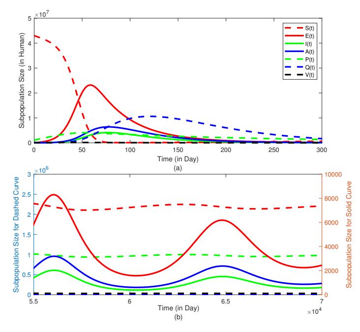
Figure 2: Numerical solution of Model (2) with parameter values in Table 2 at : (a) time interval [0,300] and (b) time interval \([5.5 \times 10^4, 7 \times 10^4]\). In (b), the left-hand side of y-axis represents a scale of solutions S(t), P(t), Q(t), and V(t), while the right-hand side of y-axis represents a scale of solutions E(t), I(t), and A(t). The solution of Model (2) subject to initial value X(0) and parameters value in Table 2 is convergent to \(\chi^*\) even though it is oscillating.
means that the average number of new exposed individual by one infected individual in susceptible and vaccinated subpopulations is 1.57. This indicates that the infection of virus SARS-CoV-2 will continue to exist. In addition, we also get the third and the fifth Routh-Hurwitz Criteria, \(\Delta_3=0.282>0\) and \(\Delta_5=1.139\times 10^{-8}>0\), respectively. This means that the endemic equilibrium point \(\chi^*\) is locally and globally asymptotically stable. The visualization for this stability is shown in Figure 2. Here, the initial value is set to be \(X(0)=(43000000,\ 1031,\ 30100,\ 20077,\ 1100000,\ 25089,\ 100225)\), which corresponds to the population size and relevant data reported by government in East Java Province, Indonesia. Figure 2(a) and 2(b) show the numerical solutions in the interval \(t\in[0,300]\) and \(t\in[5.5\times 10^4,7\times 10^4]\), respectively. It is seen that the solution oscillates but it converges to \(\chi^*\). According to Kassa et al. [21], such oscillation is caused by the asymptomatic infection, i.e., the asymptomatic infection could re-emerge the disease in the future. To verify this statement in proposed Model (2), we take \(\beta_a=0\) and then we get \(\mathcal{R}_0=0.88<1\). Hence, the disease will disappear in the future. This phenomenon is depicted in Figure 3, which shows that the disease-free equilibrium point \(\chi^{DFE1}\) of Model (2) is locally and globally asymptotically stable. Therefore, the asymptomatic infection in the epidemic model of COVID-19 has significant role, especially both \(\mathcal{R}_0\) and global stability of equilibrium points. This is in accordance with the results presented in [22].
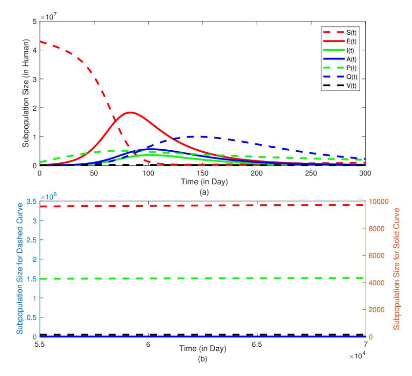
Figure 3: Numerical solution of Model (2) with parameter values in Table 2 except \(\beta_a=0\) at : (a) time interval [0,300] and (b) time interval \([5.5\times10^4,7\times10^4]\). In (b), the left-hand side of y-axis represents a scale of solutions S(t), P(t), Q(t), and V(t), while the right-hand side of y-axis represents a scale of solutions E(t), I(t), and A(t). The solution of Model (2) subject to initial value X(0) and this modified parameter value (that is, \(\beta_a=0\)) is convergent to \(\chi^{DFE1}\).
7.2. The Impact of Quarantine
The quarantine is one of COVID-19 mitigations that can reduce the size of infected subpopulations [8], [1], [31], [33], [45]. To see this effect, we take \(\gamma_4=0.4\) and \(\gamma_5=0.4\), which are twice the values of the quarantine rates in Table 2. In this case, we have \(\mathcal{R}_0=0.95<1\) and the disease-free equilibrium point \(\chi^{DFE2}(3433117, 0, 0, 0, 1527075, 0, 51597)\) is the only equilibrium point. The equilibrium point \(\chi^{DFE2}\) is locally and globally asymptotically stable. The visualization of this properties is shown in Figure 4. Notice that it is case, the COVID-19 disease will disappear in the future. This fact is caused by the increasing number of infected individuals who are quarantined such that they cannot spread COVID-19 to others. This shows that the greater quarantine rate leads to the lower basic reproduction number, which is a desirable condition for eradicating disease in future.
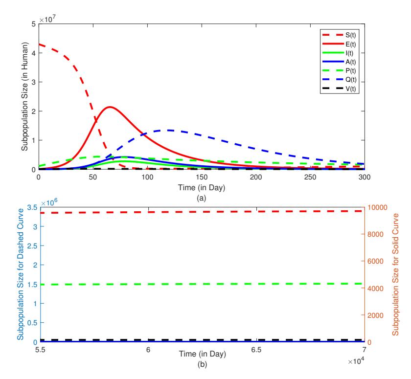
Figure 4: Numerical solution of Model (2) with parameter values in Table 2 except \(\gamma_4=0.4\) and \(\gamma_5=0.4\) at : (a) time interval [0,300] and (b) time interval \([5.5\times10^4,7\times10^4]\). In (b), the left-hand side of y-axis represents a scale of solutions S(t), P(t), Q(t), and V(t), while the right-hand side of y-axis represents a scale of solutions E(t), I(t), and I(t). The solution of Model (2) subject to initial value I(t)0 and this modified parameters value (that is, I(t)1 and I(t)3 and I(t)4 is convergent to I(t)5.
7.3. The Impact of Protection
In the proposed model (2), protected individuals are assumed to be individuals who adhere to health protocols such as wearing mask, reducing contact, wash hands routinely, and social distancing. The authors in [45], [17], [11] stated that one of the best ways to eliminate COVID-19 is to reduce contact between individuals. Based on that statement, we triple the value of protection rate in Table 2, which is \(\eta=0.045\). With this protection rate, the basic reproduction number \(\mathcal{R}_0=0.97<1\) and thus we only have the disease-free equilibrium point \(\chi^{DFE3}(2124805, 0, 0, 0, 2835386, 0, 51597)\), which is locally and globally asymptotically stable; see Figure 5.
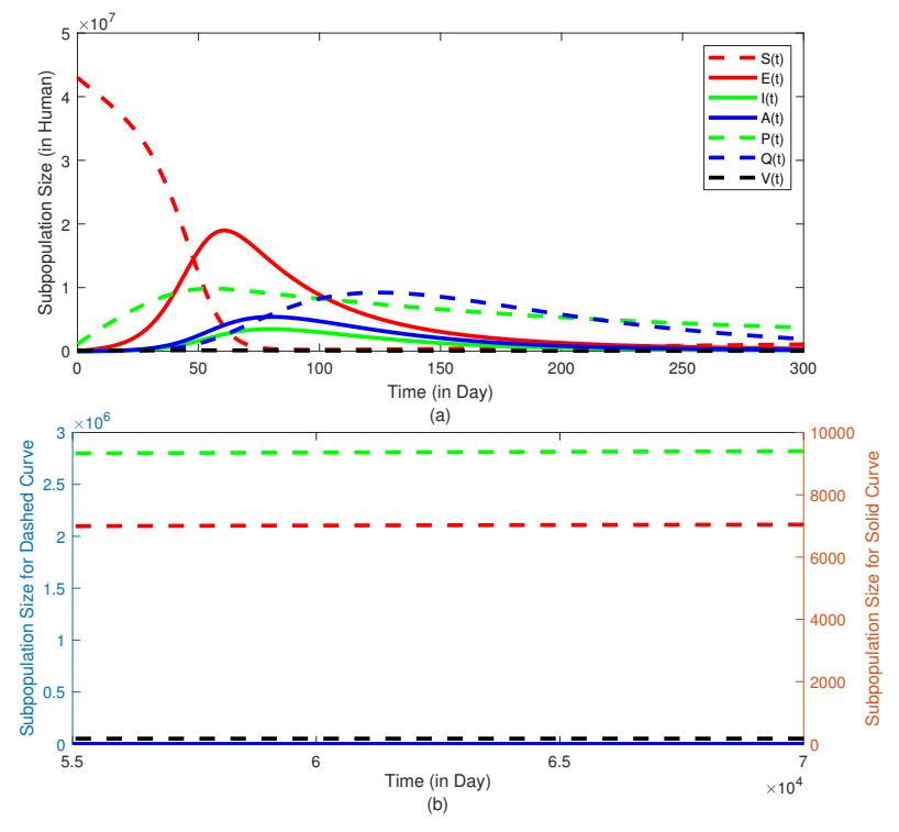
Figure 5: Numerical solution of Model (2) with parameter values in Table 2 except \(\eta=0.045\) at : (a) time interval [0,300] and (b) time interval \([5.5\times10^4,7\times10^4]\). In (b), the left-hand side of y-axis represents a scale of solutions S(t), P(t), Q(t), and V(t), while the right-hand side of y-axis represents a scale of solutions E(t), I(t), and A(t). The solution of Model (2) subject to initial value X(0) and this modified parameter value (that is, \(\eta=0.045\)) is convergent to \(\chi^{DFE3}\).
Since the protected subpopulation has no direct contact with the infected individuals, the size rate of both exposed and infected subpopulations is inversely proportional to size rate of protected subpopulation. We can see that the size of protected subpopulation is larger and the size of exposed and infected subpopulations is smaller than the case presented in Figure 2. This shows that an increase in rate of protection causes a decrease in transmission of COVID-19. Therefore, we also claim that increasing the rate of protection is strategy that can reduce the spread of COVID-19. In addition, implementing health protocols are the cost-effective strategies to control highly infected subpopulations [7].
7.4. The Impact of Vaccination
In March 2021, the vaccination program began to be implemented in East Java Province, Indonesia. Various efforts have been carried out to increase a vaccination rate by government, such as mandatory requirements for regional leaders, civil servants, health workers, and anyone involved in government administration [20]. This show that the vaccination program is a reliable COVID-19 mitigation because it can make active infections disappear in a limited time [42]. To see the impact of vaccination, we take vaccination rates \(\sigma_1 = \sigma = \frac{7}{10^4}\), which are much larger than the vaccination rates in Table 2. The basic reproduction number in this case \(\mathcal{R}_0 = 0.83 < 1\) and we do not have an endemic equilibrium point. The disease-free equilibrium point \(\chi^{DFE4}(1813187, 0, 0, 0, 798234, 0, 54329)\) is locally and globally asymptotically stable. Therefore, the increasing vaccination rates may avoid the endemic conditions. This situation is depicted in Figure 6.
In East Java Province, the most widely used vaccine types were AstraZenecca (with vaccine efficacy 70.4% during 12-week experimental period) and Sinovac (with vaccine efficacy 50.7% during 2-week experimental
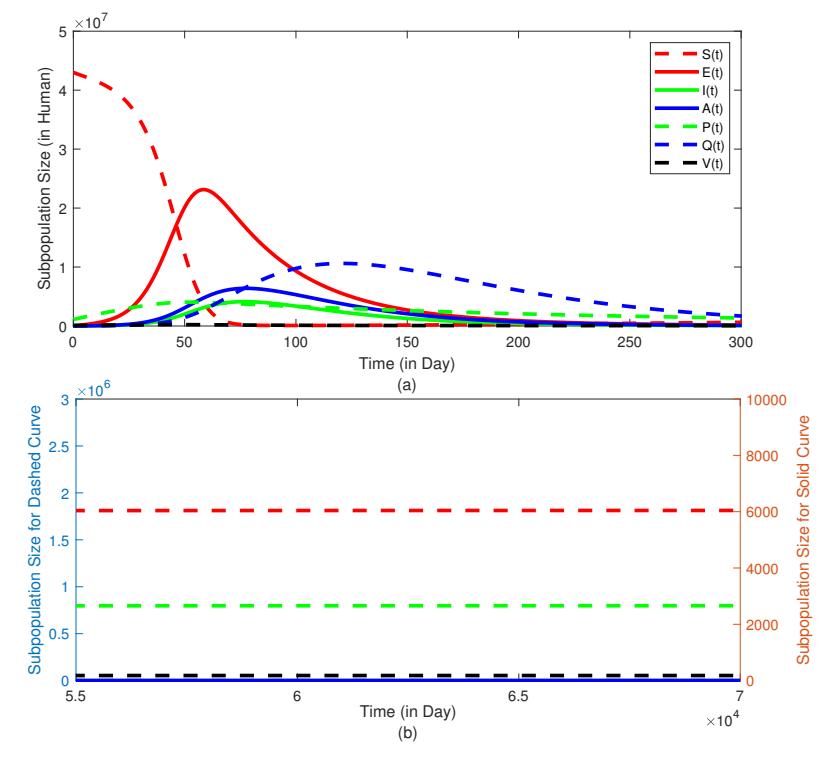
Figure 6: Numerical solution of Model (2) with parameter values in Table 2 except \(\sigma_1 = \sigma = \frac{7}{10^4}\) at : (a) time interval [0,300] and (b) time interval \([5 \times 10^4, 7 \times 10^4]\). In (b), the left-hand side of y-axis represents a scale of solutions S(t), P(t), Q(t), and V(t), while the right-hand side of y-axis represents a scale of solutions E(t), I(t), and A(t). The solution of Model (2) subject to initial value X(0) and this modified parameters value (that is, \(\sigma_1 = \sigma = \frac{7}{10^4}\)) is convergent to \(\chi^{DFE4}\).
period) [25]. If we apply parameter values as in Table 2, except \(p=0.704, q=\frac{0.704}{12\times7}\) for first scenario and \(p=0.507, q=\frac{0.507}{2\times7}\) for second scenario, then we get the basic reproduction number from both scenarios \(\mathcal{R}_0=1.59\) and \(\mathcal{R}_0=1.58\), respectively, which are almost the same as when we take p as in Table 2. This show that high vaccine efficacy has no significant effect on basic reproduction number.
8. CONCLUSION
In this paper, we introduce the new COVID-19 model by considering the asymptomatic infection and the policies such as protection (wearing mask, social distancing, and other health protocols), quarantine for infected individuals, and vaccination. The non-negativity and boundedness of solutions of the proposed model have been proven. The proposed model has two equilibrium points, that are, the disease-free equilibrium point and the endemic equilibrium point. From there, we have determined the formulation of basic reproduction number, \(\mathcal{R}_0\), using the spectral radius of next generation matrix. The local stability of equilibrium points is approximated by linearization and Jacobian Matrix. The global stability of equilibrium points is studied by defining the Lyapunov function and applying LaSalle's Invariance Principle in [28]. The disease-free equilibrium point always exists and is asymptotically stable, both locally and globally, if \(\mathcal{R}_0 < 1\). The endemic equilibrium exists uniquely and is global asymptotically stable if \(\mathcal{R}_0 > 1\). The sufficient conditions of local stability of endemic equilibrium point are more complex to be stated explicitly, that is, the third and fifth Routh-Hurwitz Criterion (see [30]). Such properties have been confirmed by numerical simulations. The simulations show that asymptomatic infections have an important role in the proposed model and the increasing of quarantine rates, protection rate, vaccination rates may cause the disappearing the COVID-19 case.
To model the spread of COVID-19, we consider the asymptomatic infections and some current government policies. For vaccination program, the increase in vaccinated community is very likely to lower the selfprotection such as wearing mask and social distancing. Therefore, it is necessary to carry out contact tracking and rapid tests into the model. We notice that hospitalization and reinfection in recovered subpopulation were not considered. This will be more interesting if these conditions are considered into the model and readjusted to the government's new policies in the future.
ACKNOWLEDGEMENT
This research was funded by FMIPA-UB via PNBP-University of Brawijaya according to DIPA-UB No. DIPA-023.17.2.677512/2021 and Contract of Professor and Doctoral Research Grant No. 1584/UN10.F09/PN/2021.