

1. INTRODUCTION
Atherosclerosis is an inflammatory disease that can be occurred when the blood vessels carry oxygen and nutrients to the rest of your body. It affects medium and large-sized arteries. The disease starts when the blood vessels become thick and stiff that is normally called hardening of the arteries. In other words, atherosclerosis is the accumulation process of fats, cholesterol and other elements in artery walls when people get older. This is commonly called plaque. The accumulation of plaque makes it difficult for blood to flow through your arteries, including around your heart, legs, and kidneys. Atheromatous plaques are appeared in the inner layers of arteries. These plaques are formed when the deposition of small cholesterol crystals started in the intima. After that the plaques are produced and bulged inside the arteries. Consequently, they reduce the blood flow. The disease starts after births and it usually a silent process. Then, it will progress during the person's life. There are several factors for the progression of this disease: hypertension, hyperlipidemia, diabetes mellitus, age, sex, smoking and life-style. Atherosclerosis is a common problem when people get older. This health problem can be treated and many successful prevention options exist [1], [2], [3].
*Corresponding Author
Most symptoms of atherosclerosis cannot be showed until a blockage occurs. There are some common symptoms: chest pain, pain in your leg, arm, and anywhere else that has a blocked artery, shortness of breath and fatigue. Atherosclerosis can cause several health problems including heart attack and stroke. Therefore, it is better to know the symptoms of both heart attack and stroke. They require immediate medical considerations and preventions [4], [5].
Atherosclerosis can be diagnosed if there are symptoms of atherosclerosis. Doctors may perform a physical exam and tests. This disease can also be treated. For example, changing lifestyle is a simple treatment in order to decrease the amount of fat and cholesterol in your body. This is how sometimes called the first line of treatment. Physical exercises are also effective treatments that may also use to improve the health of your heart and blood vessels. For some difficult cases, it may need additional medical treatments, such as medications or surgery. Medications can also help and work effectively to prevent atherosclerosis and use as treatment for infected people [6]. According to the above explanation, we can see that the number of doctors and the quality of the hospital is a crucial factor in determining the success of the atherosclerosis control strategy.
Many authors have done theoretical modeling on atherosclerosis, especially to model the mechanisms of chronic inflammation of artery walls [7], [8], [9]. Khatib et al. [7] use a reaction-diffusion model to understand the chronic inflammation of blood vessel walls. Calvez et al. [8] made a numerical approach to understanding atherosclerotic plaque formation. Silva et al. [9]continued this work using a Non-Newtonian Model of Blood Flow to model atherosclerotic Plaque Formation in the human body. Although many mathematical models have been introduced to understand atherosclerosis in the human body, not so many articles discuss the spread of this disease at the level of population dynamics. Therefore, we propose a modified atherosclerosis model from our previous work [10] by treating the hospitalization intervention as a saturated function. A routine dynamical analysis shows that our proposed model may exhibit a forward bifurcation with hysteresis or backward bifurcation at a basic reproduction number equal to one, depending on the value of the saturated parameter of the hospitalization rate. An optimal control simulation was also conducted in this article to perform some possible control strategies that may appear in a real-life situation.
2. THE MATHEMATICAL MODEL
We develop a mathematical model for atherosclerosis based on our previous work in [10], but changing the treatment rate into a saturated function to accommodate the limitation of specialist doctor to conduct surgery for infected individuals. We treat this control variable to treat the infected individual in the hospital as a timedependent variable such that we can find the best possible strategy to suppress the spread of atherosclerosis. We divide human population based on their health status and their treatment, namely susceptible human (S), Infected without treatment (I) and Infected undergo treatment (H). As one of the type of a Noncommunicable disease (NCDs), atherosclerosis do not spread through direct contact. However, social, economics and environmental condition hold an essential role in the way how these diseases spread among population. Some researchers called the infection on NCDs using the term of : "socially transmitted conditions" (STCs), which are urbanisation, industrialisation, and poverty, fast foods, alcohol and physical inactivity [11]. Hence, we assume that atherosclerosis may spread through routine social interaction between infected individuals and susceptible individuals. This approach is common to model the spread of Noncommunicable diseases (NCDs) such as diabetes, cancer, and many more [12], [13], [14], [15]. The model differential equations are given below:
\[\frac{dS}{dt} = A - \beta_1 \frac{SI}{S+I+H} - \mu S,\] \[\frac{dI}{dt} = \beta_1 \frac{SI}{S+I+H} - \frac{u(t)}{1+bI} I + \alpha H + \beta_2 \frac{IH}{S+I+H} - (\gamma + \mu) I,\] \[\frac{dH}{dt} = \frac{u(t)}{1+bI} I - \alpha H - \beta_2 \frac{IH}{S+I+H} - \mu H,\] (1)
where A present the natural recruitment rate, β1 and β2 present the infection rate of I and H, respectively, α as the progression rate, γ as death rate due to atherosclerosis, u as treatment rate, b as the half saturation parameter, and µ as the natural death rate.
Before we proceed to calculate the qualitative behavior regarding equilibrium points and the basic reproduction of the model, it is necessary to understand the basic properties of our proposed model. The following theorems state these properties.
Theorem 2.1. Given the initial condition of System (1) as follows:
\[S(t=0) > 0, I(t=0) > 0, H(t=0) > 0,\] then the solution of S(t), I(t), and H(t) from System (1) is always non-negative for all t>0.
Proof: For a non-negative initial condition, we have the following condition:
\[\begin{array}{c|ccc} \left. \frac{dS}{dt} \right|_{S=0,I\geq 0,H\geq 0} &=& A>0, \\ \left. \frac{dI}{dt} \right|_{S>0,I=0,H\geq 0} &=& \alpha H \geq 0, \\ \left. \frac{dH}{dt} \right|_{S>0,I>0,H=0} &=& \frac{u(t)}{1+bI} I \geq 0. \end{array}\]
It can be seen from the above calculation that the rates of S(t), I(t), and H(t) at the boundary of \(\mathbb{R}^3_+\) is always non-negative. Hence, we conclude that all the vector field direction goes inward from the boundary planes. Therefore, whenever the initial condition of System (1) is non-negative, then the solution will always be non-negative for all time t > 0.
Theorem 2.2. The solution of System (1) is bounded in the region
\[\Omega = \left\{ (S, I, H) \in \mathbb{R}^3_+ : S + I + H \le \frac{A}{\mu} \right\}.\]
Proof: Sum up the left and right hand sides of system (1) gives us
\[\frac{d(S+I+H)}{dt} = \frac{dN}{dt} = A - \mu(S+I+H) - \gamma I \le A - \mu N.\]
Solving \(\frac{dN}{dt} \leq A - \mu N\) with respect to N(t) yield
\[0 \le N(t) \le \frac{A}{\mu} + N(0)e^{-\mu t},\] where N(0) is a non-negative initial condition of the total population. Therefore, if the initial condition starts from the inside area of the region \(\Omega\), then the solution will stay in \(\Omega\) for \(t \to \infty\). On the other hand, if we have the initial condition starts from the outside area of the region \(\Omega\), the solution will eventually tend to \(\Omega\) as \(t \to \infty\). Hence, the proof is complete.
The main contribution here is to reduce the number of infected individual I and H using an optimal treatment rate u such that the cost of intervention can be as low as possible. This task shows minimizing the following cost function
\[\mathcal{J}(u, S, I, H) = \int_0^T \left(\omega_1 u^2 + \omega_2 I + \omega_3 H\right) dt, \tag{2}\] where \(\omega_i\) for i = 1, 2, 3 are the weight parameters, while T is the final simulation time.
3. THE DYNAMICAL BEHAVIOUR OF THE MODEL
3.1. The equilibrium points and the basic reproduction number
To analyze the dynamical behaviour of our atherosclerosis model in System (1). We consider the treatment variable as a constant parameter (u(t) = u). Hence, our model now takes the following form:
\[\frac{dS}{dt} = A - \beta_1 \frac{SI}{S+I+H} - \mu S,\] \[\frac{dI}{dt} = \beta_1 \frac{SI}{S+I+H} - \frac{u}{1+bI} I + \alpha H + \beta_2 \frac{IH}{S+I+H} - (\gamma + \mu) I,\] \[\frac{dH}{dt} = \frac{u}{1+bI} I - \alpha H - \beta_2 \frac{IH}{S+I+H} - \mu H.\] (3)
The free atherosclerosis free-equilibrium point is given by
\[\mathcal{E}_1 = (S, I, H) = \left(\frac{A}{\mu}, 0, 0\right),\tag{4}\] which represents a community without atherosclerosis. Using the next-generation matrix method [16], we develop the basic reproduction number of our proposed model in System (3). In our case, the basic reproduction number presents the number of secondary cases of atherosclerosis due to one primary atherosclerosis infection through social contact during his/her infection period in a completely susceptible population. Using a similar approach as in [16], [17], [18], [19], [20] and references therein, the basic reproduction number \((\mathcal{R}_0)\) of our model is given by
\[\mathcal{R}_0 = \frac{\beta_1(\mu + \alpha)}{\mu^2 + (\mu + \alpha + \gamma)\mu + \alpha\gamma},\tag{5}\]
which is similar with our previous work in [10]. Using results in [21], we have the following theorems.
Theorem 3.1. The atherosclerosis free equilibrium point is locally asymptotically stable when \(\mathcal{R}_0 < 1\) and unstable when \(\mathcal{R}_0 > 1\).
Theorem 3.1 represents a threshold such that community has a chance that atherosclerosis may dies out from the population. In a model where a forward bifurcation is the only possible condition at \(\mathcal{R}_0 = 1\), then we will always has a free disease condition when \(\mathcal{R}_0 < 1\). However, when a forward bifurcation is not the only possible bifurcation phenomena, then it is possible that disease still persist even though the basic reproduction number is already smaller than one. Our model shows this type of phenomena, which we will discuss later.
Theorem 3.1 show the importance of the basic reproduction number in determining the condition to guarantee the extinction of atherosclerosis from the population. Hence, it is important to know the behaviour of \(\mathcal{R}_0\) with respect to each parameter in (5), especially with controllable parameters: \(\beta_1, \alpha\), and u. Since \(\frac{\partial \mathcal{R}_0}{\partial \beta_1} = \frac{(\mu + \alpha)}{\mu^2 + (u + \alpha + \gamma)\mu + \alpha \gamma} > 0\), we know that reducing the infection rate (reduce the social interaction) will reduce \(\mathcal{R}_0\) linearly. Similarly, since \(\frac{\partial \mathcal{R}_0}{\partial \alpha} = \frac{\beta_1 u \mu}{(\mu^2 + (u + \alpha + \gamma)\mu + \alpha \gamma)^2} > 0\), then the increases of progression rate due to relapse of treated infected individual will increase \(\mathcal{R}_0\). On the other hand, since \(\frac{\partial \mathcal{R}_0}{\partial u} = -\frac{\beta_1 \mu (\mu + \alpha)}{(\mu^2 + (u + \alpha + \gamma)\mu + \alpha \gamma)^2} < 0\), then we know that increasing number of treatment rate for infected individual will increase the chance of free atherosclerosis condition in the population.
Then, we analyze the existence of the other equilibrium points. The atherosclerosis endemic equilibrium point of System (3) is given by
\[\mathcal{E}_2 = (S, I, H) = (S^*, I^*, H^*). \tag{6}\] with
\[S^* = \frac{A^2}{\mu (\beta_1 I^* + A)},\] \[H^* = \frac{u A I^*}{(\mu \beta_2 I^* + A (\alpha + \mu)) (b I^* + 1)}.\] (7)
While \(I^*\) is taken from a positive solution from the following equations:
\[f(I) = p(I)^{3} + q(I)^{2} + r(I) + s = 0,\] (8)
where p, q, r and s are expressed as follows:
\[p = b(\gamma + \mu)(\alpha \gamma \beta_{1} + \gamma \mu \beta_{1} + \gamma \mu \beta_{2})(v_{0} - 1),\] \[q = \gamma^{2} (\mu^{2} + (u + \alpha + \gamma) \mu + \alpha \gamma) + A\mu b ((\beta_{1} + \beta_{2}) \mu + \gamma \beta_{2}),\] \[+ (2 A\gamma b (\gamma + \mu) (\alpha + \mu) + (\gamma^{2} (\alpha + \mu) + \mu (u + \mu + \alpha) \gamma + Ab\beta_{2}\mu) \beta_{1} + \gamma \mu \beta_{2} (\gamma + \mu)),\] \[(w_{0} - 1)\] \[r = A (\gamma + \mu) ((Ab + \beta_{2}) \mu + A\alpha b) + (2 A (\mu^{2} + (u + \alpha + \gamma) \mu + \alpha \gamma) \gamma + A\beta_{1} (Ab (\alpha + \mu) + \mu \beta_{2})),\] \[(z_{0} - 1)\] \[s = A^{2} (\mu^{2} + (u + \alpha + \gamma) \mu + \alpha \gamma) (1 - \mathcal{R}_{0}).\] and
\[v_{0} = \frac{\alpha \gamma^{2} + \gamma^{2} \mu + \mu \beta_{1} \beta_{2}}{\alpha \gamma \beta_{1} + \gamma \mu \beta_{1} + \gamma \mu \beta_{2}},\] \[w_{0} = \frac{2 A \alpha b \gamma \beta_{1} + A \alpha b \mu \beta_{1} + 2 A b \gamma \mu \beta_{1} + A b \mu^{2} \beta_{1} + \gamma \mu \beta_{1} \beta_{2} + \mu^{2} \beta_{1} \beta_{2}}{2 A \gamma b (\gamma + \mu) (\alpha + \mu) + (\gamma^{2} (\alpha + \mu) + \mu (u + \mu + \alpha) \gamma + A b \beta_{2} \mu) \beta_{1} + \gamma \mu \beta_{2} (\gamma + \mu)},\] \[z_{0} = \frac{A \beta_{1} (\mu^{2} + (u + \alpha + 2 \gamma) \mu + 2 \alpha \gamma)}{2 A \gamma (\mu^{2} + (u + \alpha + \gamma) \mu + \alpha \gamma) + A (A b (\alpha + \mu) + \mu \beta_{2}) \beta_{1}}.\]
The following theorem states the existence of at least one endemic equilibrium when \(\mathcal{R}_0 > 1\).
Theorem 3.2. System (3) always has at least one endemic equilibrium when \(\mathcal{R}_0 > 1\).
Proof: From the expression of p and s, it is clear that \(p>0 \iff \beta_1>\beta_1^*=\gamma\), and \(s<0 \iff \mathcal{R}_0>1 \iff \beta_1>\beta_1^{**}=\gamma+\frac{\alpha\mu+\mu^2+\mu u}{\mu+\alpha}\). From this expression, it is easy to see that whenever \(\mathcal{R}_0>1\), then we always have p>0 and s<0.
When \(\mathcal{R}_0=1\), then we have s=0 which means that polynomial f(I) has exactly one zero root. Furthermore, since p>0, then we have that \(\lim_{I\to\infty} f(I)=\infty\) and \(\lim_{I\to-\infty} f(I)=-\infty\). Hence, when we have \(\mathcal{R}_0>1\), then we have s<0 which will shift f(I) downward. Hence, we have at least one positive root of f(I) when \(\mathcal{R}_0>1\).
Now, we analyze the possible existence of another positive equilibrium when \(\mathcal{R}_0 < 1\). The following theorem guarantee the existence of at least one atherosclerosis endemic equilibrium point when \(\mathcal{R}_0 < 1\).
Theorem 3.3. System (3) has at least one endemic equilibrium when \(\mathcal{R}_0 < 1\) if \(b > b^*\) where
\[b^* = \frac{(u+\mu+\alpha)\left(\mu^2 + (u+\alpha+\gamma)\mu + \alpha\gamma\right) - \mu u\beta_2}{A\alpha u + A\mu u}.\] (9)
Proof: We prove this theorem using a gradient analysis of f(I) at I=0 and \(\mathcal{R}_0=1\). At first, we set p as a function of \(\mathcal{R}_0\) by setting \(\beta_1\) as the bifurcation parameter and substitute it to each coefficient of f(I). Solving \(\mathcal{R}_0\) with respect to \(\beta_1\), and substitute it to f(I), then we have each coefficient on f(I) as a function of \(\mathcal{R}_0\) as follows.
\[p(\mathcal{R}_0)I^3 + q(\mathcal{R}_0)I^2 + r(\mathcal{R}_0)I + s(\mathcal{R}_0) = 0.\]
Taking the implicit derivative of above equation with respect to \(\mathcal{R}_0\), we have
\[\frac{\partial p}{\partial \mathcal{R}_0} I^3 + p(\mathcal{R}_0) 3I \frac{\partial I}{\partial \mathcal{R}_0} + \frac{\partial q}{\partial \mathcal{R}_0} I^2 + q(\mathcal{R}_0) 2I \frac{\partial I}{\partial \mathcal{R}_0} + \frac{\partial r}{\partial \mathcal{R}_0} I + r(\mathcal{R}_0) \frac{\partial I}{\partial \mathcal{R}_0} + \frac{\partial s}{\partial \mathcal{R}_0} = 0.\]
Substitute I=0 and \(\mathcal{R}_0=1\) to above equation, and solve it with respect to \(\frac{\partial I}{\partial \mathcal{R}_0}\) gives us
\[\frac{\partial I}{\partial \mathcal{R}_0} = A^2 \left( \alpha \gamma + \alpha \mu + \gamma \mu + \mu^2 + \mu u \right) \frac{1}{r},\] where \[r = -\frac{A\mu}{\mu+\alpha} \left( b(A\alpha u + A\mu u) + \mu u\beta_2 - (u+\mu+\alpha) \left( \mu^2 + (u+\alpha+\gamma) \mu + \alpha \gamma \right) \right)\].
From above analysis, we know that f(I) will have at least one positive root when \(\frac{\partial I}{\partial \mathcal{R}_0} < 0\) which equivalent to a condition when r < 0. Therefore, we have that r < 0 if and only if
\[b > b^* = \frac{(u + \mu + \alpha)(\mu^2 + (u + \alpha + \gamma)\mu + \alpha\gamma) - \mu u\beta_2}{A\alpha u + Auu}.\]
Hence, the proof is complete.
From the expression of \(\mathcal{R}_0\), we can see that \(\mathcal{R}_0\) is not depend on \(\beta_2\) and b. However, Theorem 3.3 shows us that these two parameters will determine a condition when an endemic equilibrium may still persist even \(\mathcal{R}_0 < 1\). Theorem 3.3 shows how b may trigger multiple endemic equilibriums if \(b > b^*\). Using the same formula, but choosing \(\beta_2\) as the critical parameter will give us a condition of multiple endemic equilibriums depend on \(\beta_2\). To be precise, the critical value of \(\beta_2\) is given by
\[\beta_2^* = \frac{b(A\alpha u + A\mu u) - (u + \mu + \alpha)\left(\mu^2 + (u + \alpha + \gamma)\mu + \alpha\gamma\right)}{\mu u}.\] (10)
Hence, if \(\beta_2 > \beta_2^*\), then we will have at least one endemic equilibrium when \(\mathcal{R}_0 < 1\). Therefore, reducing the spread of atherosclerosis by only paying attention in reducing \(\mathcal{R}_0\) without concerning to the number of doctors (b) or secondary infection \((\beta_2)\) is not wise, since it may trigger a complex condition in the field.
Next, we use Descartes rules of sign to analyze the possible number of endemic equilibrium when \(\mathcal{R}_0 < 1\) and \(\mathcal{R}_0 > 1\). The result is given in Table 1. We can see that it is possible that we have two endemic equilibriums when \(\mathcal{R}_0 < 1\), or even three endemic equilibriums when \(\mathcal{R}_0 > 1\).
| Case | p | q | r | s | \(\mathcal{R}_0\) | Change of sign | Possible roots |
|---|---|---|---|---|---|---|---|
| 1 | + | + | + | + | \(\mathcal{R}_0 < 1\) | 0 | 0 |
| 2 | + | + | + | - | \(\mathcal{R}_0 > 1\) | 1 | 1 |
| 3 | + | + | - | + | \(\mathcal{R}_0 < 1\) | 2 | 0 or 2 |
| 4 | + | + | - | - | \(\mathcal{R}_0 > 1\) | 1 | 1 |
| 5 | + | - | + | + | \(\mathcal{R}_0 < 1\) | 2 | 0 or 2 |
| 6 | + | - | + | - | \(\mathcal{R}_0 > 1\) | 3 | 1 or 3 |
| 7 | + | - | - | + | \(\mathcal{R}_0 < 1\) | 2 | 0 or 2 |
| 8 | + | - | - | - | \(\mathcal{R}_0 > 1\) | 1 | 1 |
Table 1: Possible number of positive roots of f(I).
From Theorem 3.2 and 3.3, our model suggests that atherosclerosis may still exist even though \(\mathcal{R}_0\) is already smaller than one. This result means that the basic reproduction number no longer can be the unique indicator to determine whether atherosclerosis may still exist or dies out. Therefore, to analyze the qualitative behaviour on the dynamic of System (3), we conduct our bifurcation analysis in the following section.
3.2. Existence of forward bifurcation with hysteresis
In this chapter, we analyze the bifurcation of System (3) using the well known Castillo-Song bifurcation theorem [22] at \(\mathcal{R}_0 = 1\). Let
\[S = x_1, \quad I = x_2, \quad H = x_3,\]
\[\frac{dS}{dt} = g_1, \quad \frac{dI}{dt} = g_2, \quad \frac{dH}{dt} = g_3.\]
Hence, System (3) becomes as follows:
\[g_{1} = A - \beta_{1} \frac{x_{1}x_{2}}{x_{1} + x_{2} + x_{3}} - \mu x_{1},\] \[g_{2} = \beta_{1} \frac{x_{1}x_{2}}{x_{1} + x_{2} + x_{3}} - \frac{u}{1 + bx_{2}} x_{2} + \alpha x_{3} + \beta_{2} \frac{x_{2}x_{3}}{x_{1} + x_{2} + x_{3}} - \gamma x_{2} - \mu x_{2},\] \[g_{3} = \frac{u}{1 + bx_{2}} x_{2} - \alpha x_{3} - \beta_{2} \frac{x_{2}x_{3}}{x_{1} + x_{2} + x_{3}} - \mu x_{3}.\] (11)
First, we have to check the existence of zero eigenvalue of linearized System (11) at \(\mathcal{R}_0 = 1\) and \(\mathcal{E}_1\) such that we can use center-manifold theory to conduct further analysis. Therefore, let us choose \(\beta_1\) as the bifurcation parameter. Solving \(\mathcal{R}_0\) with respect to \(\beta_1\), we have
\[\beta_1 = \beta_1^{\dagger} = \frac{\left(\alpha \gamma + \alpha \mu + \gamma \mu + \mu^2 + \mu u\right)}{\mu + \alpha}.\] (12)
Linearized System (11) at \(\mathcal{R}_0 = 1\) and \(\mathcal{E}_1\), we have
\[\boldsymbol{J}|_{\mathcal{E}_{1},\beta_{1}} = \begin{bmatrix} -\mu & \frac{-\mu^{2} + (-u - \alpha - \gamma)\mu - \alpha \gamma}{\alpha + \mu} & 0\\ 0 & -\frac{u\alpha}{\alpha + \mu} & \alpha\\ 0 & u & -\alpha - \mu \end{bmatrix}.\](13)
This matrix has three eigenvalues, i.e. \(\lambda_1=0, \lambda_2=-\mu\) and \(\lambda_3=-\frac{\alpha^2+2\mu\alpha+u\alpha+\mu^2}{\alpha+\mu}\). Since we have simple zero eigenvalue and the others are negative, then we can use center manifold theory to analyze the bifurcation of our model. Then, we calculate the right and left eigenvectors respected to the zero eigenvalue. The right eigenvectors of the zero eigenvalue, namely \(\vec{w}=(w_1,w_2,w_3)\) is given by
\[w_1 = -\frac{\left(\alpha\gamma + \mu\alpha + \gamma\mu + \mu^2 + u\mu\right)w_3}{\mu u},\]
\[w_2 = \frac{\left(\alpha + \mu\right)w_3}{u},\]
\[w_3 = 1.\]
On the other hand, the left eigenvector, namely \(\vec{v} = (v_1, v_2, v_3)\), is given by:
\[v_1 = 0,\] \[v_2 = \frac{(\alpha + \mu) v_3}{\alpha},\] \[v_3 = 1.\]
Since \(v_1 = 0\), then we do not need to calculate the partial derivative of \(g_1\). Hence, the partial derivative of \(g_2\) and \(g_3\) are given by:
\[\begin{split} &\frac{\partial^2 g_2}{\partial x_2^2} = -2 \, \frac{\left(\mu^2 + (\alpha + \gamma + u) \, \mu + \alpha \, \gamma\right)}{\left(\alpha + \mu\right) \, x_1} + 2 \, ub, \\ &\frac{\partial^2 g_2}{\partial x_2 \partial x_3} = \frac{\partial^2 g_2}{\partial x_3 \partial x_2} = -\frac{\left(\mu^2 + (\alpha + \gamma + u) \, \mu + \alpha \, \gamma\right)}{\left(\alpha + \mu\right) \, x_1} + \frac{\beta_2}{x_1}, \\ &\frac{\partial^2 g_2}{\partial x_2 \partial \beta_1} = \frac{\partial^2 g_2}{\partial \beta_1 \partial x_2} = 1, \quad \frac{\partial^2 g_3}{\partial x_2^2} = -2 \, u \, b, \quad \frac{\partial^2 g_3}{\partial x_2 \partial x_3} = \frac{\partial^2 g_3}{\partial x_3 \partial x_2} = -\frac{\beta_2}{x_1}. \end{split}\]
By using the formula of A and B in [22], we have
\[\begin{split} \mathcal{A} &= \sum_{k,i,j=1}^{3} v_k w_i w_j \frac{\partial^2 g_k}{\partial x_i \partial x_j}(0,0) \\ &= 2 \frac{\mu \left(\alpha + \mu\right)}{A u^2 \alpha} \left( u \, b A \alpha + u \, b A \mu - \left( \left(\mu^2 + \left(u + \alpha + \gamma\right) \mu + \alpha \, \gamma\right) \left(\alpha + \mu + u\right) \right) + \mu \, u \beta_2 \right), \end{split}\] and
\[\mathcal{B} = \sum_{k,i=1}^{3} v_k w_i \frac{\partial^2 g_k}{\partial x_i \partial \beta_1} (0,0),\] \[= v_2 w_2 \frac{\partial^2 g_2}{\partial x_2 \partial \beta_1},\] \[= \left( \frac{(\alpha + \mu) v_3}{\alpha} \right) \left( \frac{(\alpha + \mu) w_3}{u} \right) (1),\] \[= \frac{(\alpha + \mu)^2}{\alpha^2 u} > 0,\]
It can be seen that \(\mathcal{B}\) is always positive, while \(\mathcal{A}\) can be positive or negative. Hence, the type of bifurcation that may appear is depend on the sign of \(\mathcal{A}\) as follows:
1) A > 0 if and only if
\[ubA\alpha + ubA\mu + \mu u\beta_2 > (\mu^2 + (u + \alpha + \gamma)\mu + \alpha\gamma)(\alpha + \mu + u). \tag{14}\] 2) A < 0 if and only if
\[ubA\alpha + ubA\mu + \mu u\beta_2 < (\mu^2 + (u + \alpha + \gamma)\mu + \alpha\gamma)(\alpha + \mu + u). \tag{15}\]
Based on above results, we have the following theorem.
Theorem 3.4. System (3) undergoes a forward bifurcation phenomena when \(b < b^*\), and backward bifurcation when \(b > b^*\), where
\[b^* = \frac{(u + \mu + \alpha) (\mu^2 + (u + \alpha + \gamma) \mu + \alpha \gamma) - \mu u \beta_2}{A\alpha u + A\mu u}.\]
3.3. Numerical simulations on the type of bifurcation
To conduct numerical experiment on this section, we use the following parameter values: \(A = \frac{1000}{65 \times 365}\), \(\alpha = 10^{-5}\), \(\beta_2 = 0.2\), \(\gamma = 10^{-3}\), u = 0.2, \(\mu = \frac{1}{65 \times 365}\) while \(\beta_1\) and b are various. Using these parameter values, we have that \(\mathcal{R}_0 = 1\) when \(\beta_1 = 0.162\). Furthermore, we have that \(b^*\) in Theorem 3.4 is 0.025. The bifurcation diagram of System (3) have shown in Figure 1 based on different value of b.
The first bifurcation type is a forward bifurcation as shown in Figure 1a, when we choose \(b = 10^{-4} < b^*\). We can see that we have the atherosclerosis free equilibrium is always stable when \(\mathcal{R}_0 < 1\), and unstable when \(\mathcal{R}_0 > 1\). On the other hand, we only have one stable endemic equilibrium when \(\mathcal{R}_0 > 1\), and no endemic equilibrium otherwise. This means that, larger capacity of the hospital (smaller b) will reduce the possibility of misinterpretation of endemics in the field, and atherosclerotic disease is easier to control.
When we choose \(b=0.05>b^*\), then according to Theorem 3.4, we will have System (3) undergoes a backward bifurcation at \(\mathcal{R}_0=1\) as shown in Figure 1b. In this situation, it is still possible to reach a disease free state when \(\mathcal{R}_0<1\). However, it is also possible that the final condition when \(\mathcal{R}_0<1\) will end up in an endemic state depend on the initial condition of System (3). To be precise, we have two endemic equilibriums when \(\mathcal{R}_0<1\), one of them is stable and the other is unstable. When \(\mathcal{R}_0>1\), we have a higher values of the endemic equilibrium.
The last possible bifurcation type is the forward bifurcation with hysteresis. This condition is obtained when the value of b is not significantly smaller than \(b^*\), which in our case we take \(b = 2 \times 10^{-3} < b^*\). As we can see from Figure 1c, we have a complex situation around \(\mathcal{R}_0 = 1\). When \(\mathcal{R}_0 > 1\), but close to 1, we have three endemic equilibriums, two of them are stable, while the other one is unstable. On the other hand, when \(\mathcal{R}_0 < 1\) but close to one, we have a similar qualitative result with a backward bifurcation, where we have one stable endemic equilibrium and one unstable endemic equilibrium. This phenomena is not appears often in epidemiological model. Readers can see [23] for further discussion about this idea.
From these numerical experiments, it can be concluded that controlling atherosclerosis is much more difficult when there are limited health facilities, both hospitals and doctors, because the emergence of backward bifurcation and forward bifurcation with hysteresis can trigger difficulties in predicting the final state in the field. This is because the existence of the basic reproduction number is no longer the only indicator for the endemicity of the proposed model.
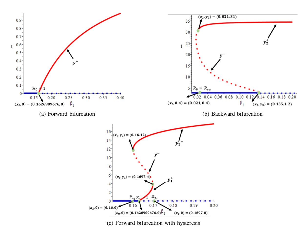
Figure 1: Three types of possible bifurcation phenomena of atherosclerosis model in (3).
4. OPTIMAL CONTROL SIMULATION
In this section, we carry out a numerical characterization and simulation of the optimal control problem for System (1) where the corresponding cost function is given by (2). We start by performing the characterization of the optimal control problem using the Pontryagin Maximum Principle (PMP) [24], and followed with some numerical experiments.
4.1. Characterization of the optimal control problem
As we mentioned before, we characterize our optimal control problem using the well-known Pontryagin's Maximum Principle (PMP) [24] to determine the optimality condition of treatment rate u(t). The Lagrangian of System (1) is defined as
\[\mathcal{L}(S, I, H, u, \lambda_{i}, \omega_{i}) = \omega_{1}u^{2} + \omega_{2}I + \omega_{3}H + \lambda_{1}\frac{dS}{dt} + \lambda_{2}\frac{dI}{dt} + \lambda_{3}\frac{dH}{dt}, = \omega_{1}u^{2} + \omega_{2}I + \omega_{3}H ... + \lambda_{1}\left[A - \beta_{1}\frac{SI}{S + I + H} - \mu S\right]... + \lambda_{2}\left[\beta_{1}\frac{SI}{S + I + H} - \frac{u(t)}{1 + bI}I + \alpha H + \beta_{2}\frac{IH}{S + I + H} - (\gamma + \mu)I\right]... + \lambda_{3}\left[\frac{u(t)}{1 + bI}I - \alpha H - \beta_{2}\frac{IH}{S + I + H} - \mu H\right],\] (16)
where \(\lambda_i\) for i = 1, 2, 3 are the adjoint variables for S, I, and H, respectively, while \(\omega_i\) for i = 1, 2, 3 are the weight parameters.
The adjoint variables \(\lambda_1, \lambda_2\) and \(\lambda_3\) satisfy the following conditions:
\[\frac{d\lambda_{1}}{dt} = -\frac{\partial \mathcal{L}}{\partial S}, = \beta_{1}I \left( \frac{I+H}{(S+I+H)^{2}} \right) (\lambda_{1} - \lambda_{2}) + \mu\lambda_{7}, \frac{d\lambda_{2}}{dt} = -\frac{\partial \mathcal{L}}{\partial I}, = -\omega_{2} + \beta_{1}S \left( \frac{S+H}{(S+I+H)^{2}} \right) (\lambda_{2} - \lambda_{1}) + (\mu + \gamma)\lambda_{2} \dots + \left[ \frac{u}{(1+bI)^{2}} - \beta_{2}H \left( \frac{S+H}{(S+I+H)^{2}} \right) \right] (\lambda_{3} - \lambda_{2}), \frac{d\lambda_{3}}{dt} = -\frac{\partial \mathcal{L}}{\partial H}, = -\omega_{3} + \beta_{1} \frac{SI}{(S+I+H)^{2}} (\lambda_{2} - \lambda_{1}) + \beta_{2}I \left[ \left( \frac{S+I}{(S+I+H)^{2}} \right) + \alpha \right] (\lambda_{3} - \lambda_{2}) + \mu\lambda_{3},\] (17)
with a transversality condition \(\lambda_i(T)=0\) for i=1,2,3. Solving \(\frac{\partial \mathcal{L}}{\partial u}=0\) with respect to u, we have
\[u = \frac{1}{2\omega_1} \frac{I}{1 + bI} (\lambda_2 - \lambda_3).\]
Combining above u with associated lower bound \(u^{\min}\) and upper bound \(u^{\max}\), we have the optimal control of \(u^*\) is given by
\[u^* = \min\left\{u^{\max}, \max\left\{u^{\min}, \frac{1}{2\omega_1} \frac{I}{1+bI}(\lambda_2 - \lambda_3)\right\}\right\}.\] (18)
4.2. Numerical experiments
We use the Fourth-order of Runge-Kutta Method to solve our optimal control problem numerically. The problem consists of the disease model in (1), cost function in (2), adjoint system in (17) with transversal condition, and optimal condition in (18). Using an initial guess of u for all \(t \in [0,T]\), we start our computation by solving the atherosclerosis model in System (1) forward in time since we have initial condition of S,I, and H are given. Next, we solve our adjoint system in (17) backward in time using the transversal condition. We update our control in (18) using the previous numerical calculation on state and adjoint variables, and update it until the convergence criteria is achieved. Please see [25], [26] for further examples of the implementation of this numerical algorithm to solve the optimal control problem from the epidemiological models. To conduct the numerical simulations, we use the following parameter values: \(A = \frac{1000}{65 \times 365}, \beta_1 = 0.2, \beta_2 = 0.1, \mu = \frac{1}{65 \times 365}, b = 0.005, \alpha = 0.0005\), and \(\gamma = 0.0001\) which give us \(\mathcal{R}_0 > 1\) withoutcontrol implemented.
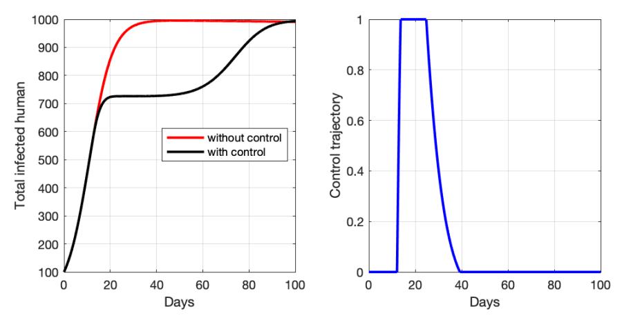
Figure 2: Optimal control simulations for scenario-1.
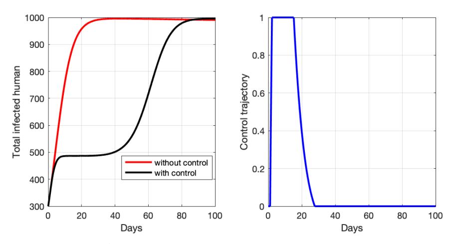
Figure 3: Optimal control simulations for scenario-2.
The first numerical simulation (scenario-1) conducted when the total number of infected individuals is only 10% from the population. The result is given in Figure 2. We can see that the control is given only for a short time period in day 13 until day 24, and tends to zero rapidly in the next days. With this control profile, we can see that the total number of infected individuals stop to increase at day-13, and continue to increase as soon as the control intervention stopped. The cost function for this scenario is 1526, 72.
For the second scenario (scenario-2), we perform our numerical experiment with different initial values used in scenario-1. In this scenario, we assume that 30% of total population is already infected by atherosclerosis. The result is given in Figure 3. Due to the high number of infected individuals at the start of the simulation, maximum intensity of control should be given for the first 18 days, before decreasing to zero the very next day of simulation. Therefore, we can see that number of infected individuals can be suppressed early on, before increasing again when the control disappears. The cost function for this simulation is 1663, 16. This cost function is higher than scenario-1, since the control reaches its maximum effect sooner and lasts longer in scenario-2. Therefore, we can conclude from these numerical experiments that giving control in a endemic prevention (scenario-1) has a lower cost of intervention then for an endemic reduction scenario (scenario-2).
5. CONCLUSIONS
This paper discussed the mathematical model of atherosclerosis with limited hospital resources. The intervention of hospitalization takes place in the model to reduce the death rate of atherosclerosis. Disease-free equilibrium and the basic reproduction number were found analytically, and we concluded that atherosclerosis can be eliminated from the population when the basic reproduction number is less than one. Numerical results show that it is possible to have a multiple endemic equilibrium when the basic reproduction number is less than one (backward bifurcation), or larger than one (forward bifurcation with hysteresis), depending on the saturation parameter of the hospitalization rate or the infection rate of treated infected individuals. These results indicate that controlling atherosclerosis should consider not only the value of the basic reproduction number, but also the quality of hospitalization intervention (maximum capacity of the hospital, availability of the doctor, etc). Furthermore, some numerical experiments on the optimal control problem indicated that the endemic prevention scenario is more easily (i.e. less costly) than the endemic reduction scenario.
ACKNOWLEDGEMENT
This research is funded by Indonesian RistekBRIN with PDUPT research grant scheme (ID Number: NKB-159/UN2.RST/HKP.05.00/2021), 2021.