1. INTRODUCTION

The coronavirus belongs to the family of viruses that causes respiratory and intestinal illnesses in humans and animals ([1], [2]). It leads to coronavirus disease in 2019 with accepted acronym COVID-19 worldwide. It results to fatality of millions of people and economic meltdown of many countries. The COVID-19 pandemic has created global anxiety that cut across Africa, Asia, Europe, America and other continents in the world. Non-African countries have had the worst hit of COVID-19 in the first quarter of the year 2020. It was estimated that 99.2% of the global total of 3,090,445 million people with COVID-19 lived in continents outside Africa [3]. People dying more from the disease comes from those with chronic co-morbidities such as cardio vascular and cerebra-vascular diseases, diabetes, hepatitis B virus and other infections [4]. Findings about the disease characteristics are rapidly changing and subject to selection bias. Incubation period has been found to be long as 19 or 24 days, beyond the 14 days window period, which has been a baseline of case definition [5]. Up till now, the spread and transmission of the disease rely heavily on human to human contact with human infected droplets, blood and infected objects. Apart from the index case in Wuhan, exposed immigrants (infected but without symptoms) have been the key drivers of the present COVID-19 pandemic and past epidemics ([6], [7], [8]). About 44% cases of COVID-19 due to pre-symptomatic transmission are widely reported [9]. In particular, 201 cases of coronavirus through pre-symptomatic and asymptomatic transfer were reported in Azad Jammu and Kashmir [10]. No nation in the world today apart from China has an index case of COVID-19 independent of exposed immigrants.

From the beginning of COVID-19 to date, a couple of mathematical models as indispensable tool have been constructed and applied in gaining better understanding on the spread and transmissibility, impacts of preventive and curative strategies of the disease. For example, see [11], [12] for details on general dynamics of COVID-19. Some works focus on testing and detection [13]. Some implements the use of vaccines [14] and others focus on influence of infective immigrants [15], quarantine and education ([16], [17]), lockdown,

^*Corresponding author

contact tracing and isolation ([18], [19]). Research in these areas have presented novel results on preventive and curable steps to contain the pandemic and have reported better outcomes in terms of completing time estimation for contact tracing. However, a robot form of models with a justifiable and satisfactory assessment is needed. In all the authors cited above, none of them has consider the impact of exposed immigrants (who escapes quarantine undetected at the point of entry) on the spread of COVID-19. It is on this plight that the present study proposes a mathematical model of COVID-19 transmission dynamics in the presence of exposed immigrants.

The rest of the paper is organized as follows: In Section 2, we present the model formulation and analysis of the model in Section 3. Simulations and discussion are given in Section 4. Section 5 deals with the conclusion of the paper.

2. MODEL FORMULATION

A population size denoted by N(t) at any time t with constant inflow of susceptibles at a rate \(\pi_s\) is examined. The total population is partitioned into four classes of susceptible (S), exposed (E), Quarantined \((Q_1)\), and isolated/hospitalized \((Q_2)\) individuals. Apart from the first case in Wuhan, China, we assume that all cases of COVID-19 in other countries were as a result of having contact with the exposed immigrants. Exposed individuals here are either asymptomatic or pre-symptomatic but infectious. \(Q_1\) are both locals and exposed immigrants that follow legal routes (airports) on their arrival while \(Q_2\) are infected individuals with symptoms isolated for treatment. Individuals in classes \((Q_1)\) and \((Q_2)\) are assumed not to be transmitting the disease since they are confined for symptoms observation and treatment respectively. Therefore, their interactions with the general susceptible population is negligible. The study does not consider a separate class for infectious people since they are placed under class \((Q_2)\) as required by the medical guidelines on COVID-19 prevention and treatment [20]. It is also assumed that exposed individuals do not die of COVID-19. In all classes, they experience a natural death rate, \(\mu\) and the COVID-19 induced death rate, \(\delta\) specified for the isolated individuals \((Q_2)\). The exposed individuals recover at a rate, \(\gamma_1\) by body immune system while \(\gamma_2\) remains the recovery rate of the hospitalized individuals due to treatment. Furthermore, \(\beta\) is the rate of exposure to the coronavirus that results to infection and \(\alpha\) is the number of exposed individuals that had contact with the susceptible individuals. As in [22], we introduce the immigrants who are exposed to the coronavirus as thus: \(q_1mE\) is the recruitment of exposed immigrants into the quarantine class at point of entry through legal routes and \(q_2mE\) is a complementary proportion of immigrants that escapes quarantine undetected into the exposed class, where m is the rate of influx of exposed immigrants. Apart from the quarantining of immigrants, individuals who are exposed within the community are also quarantined internally at rate \(\nu\). After being in the quarantine class for 14 days, those individuals without the symptoms of the disease are released to the susceptible class at a rate, \(\xi\) and individuals with clinical symptoms are isolated at a rate, \(\omega_1\). The exposed individuals develop symptoms of the disease are therefore isolated at rate, \(\omega_2\). We assumed that isolated individuals recover to gain susceptibility at a rate, \(\gamma_2\). It is also assumed that the interactions between susceptible and exposed individual follows a standard incidences function as given in the flow diagram of the model. In view of these assumptions and schematic diagram in Figure 1, we derive the following differential equations in System (1).

\[\begin{split} \frac{dS}{dt} &= \pi_s + \xi Q_1 + \gamma_1 E + \gamma_2 Q_2 - \frac{\beta \alpha ES}{N} - \mu S, \\ \frac{dE}{dt} &= \frac{\beta \alpha ES}{N} + q_2 mE - (\mu + \nu + \gamma_1 + \omega_2) E, \\ \frac{dQ_1}{dt} &= (q_1 m + \nu) E - (\mu + \xi + \omega_1) Q_1, \\ \frac{dQ_2}{dt} &= \omega_1 Q_1 + \omega_2 E - (\mu + \delta + \gamma_2) Q_2, \end{split} \tag{1}\]

with

\[S(0) = S^0, E(0) = E^0, Q_1(0) = Q_1^0, Q_2(0) = Q_2^0\] and \(q_2 = 1 - q_1\).

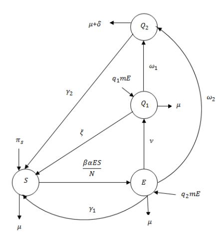
Figure 1: Schematic diagram of COVID-19 transmission dynamics with exposed immigrants.

Adding the entire equations of the system (1) accounts for the differential equation (2)

\[\frac{dN}{dt} = \pi_s - \mu N - \delta Q_2 + mE,\tag{2}\]

where \(N=S+E+Q_1+Q_2\). For a system free from influx of exposed immigrants (m=0), Equation (2) becomes \(\frac{dN}{dt} \leq \pi_s - \mu N\). Therefore, as in [12], it can be shown that \(\limsup N(t)_{t\longrightarrow\infty} \leq \frac{\pi_s}{\mu}\). Thus, the invariant set for model (1) is

\[\Upsilon = \{ (N, E, Q_1, Q_2) \in R_+^4 : N + E + Q_1 + Q_2 \le \frac{\pi_s}{\mu}, N > 0, E \ge 0, Q_1 \ge 0, Q_2 \ge 0 \}.\]

Without loss of generality, the system (1) can be rewritten as:

\[\frac{dN}{dt} = \pi_s - \mu N - \delta Q_2 + mE, \frac{dE}{dt} = \beta \alpha (N - E - Q_1 - Q_2) \frac{E}{N} + q_2 mE - (\mu + \nu + \gamma_1 + \omega_2) E, \frac{dQ_1}{dt} = (q_1 m + \nu) E - (\mu + \xi + \omega_1) Q_1, \frac{dQ_2}{dt} = \omega_1 Q_1 + \omega_2 E - (\mu + \delta + \gamma_2) Q_2.\] (3)

Continuity of the right-hand side of Equation (3) and its derivative implies the model is biologically well behaved.

3. MODEL ANALYSIS

3.1. Basic reproduction number \((R_0)\)

To obtain a COVID-19-free equilibrium, it is expected that the entire population is to be occupied by susceptibles and devoid of the other classes (i.e. all other classes go to extinction after some time). Following the work in [22], we set S=N and \(E=Q_1=Q_2\) considered to be zero in a situation where few infectives dominate the population. This is then substituted into the differential coefficient of exposed class to obtain

\[\frac{dE}{dt} = [\beta \alpha + q_2 m - (\mu + \nu + \gamma_1 + \omega_2)]E. \tag{4}\]

Since Equation (4) is a variable separable differential equation, we get by integration

\[E(t) = E_0 exp[(\beta \alpha + q_2 m - (\mu + \nu + \gamma_1 + \omega_2))t].\]

If \(\beta\alpha + q_2m - (\mu + \nu + \gamma_1 + \omega_2) < 0\), then the number of exposed diminishes exponentially with time. Therefore, exposure to COVID-19 at infinity (i.e. \(t \longrightarrow \infty\)) becomes minimal. Interestingly, if

\[\beta\alpha + q_2m - (\mu + \nu + \gamma_1 + \omega_2) < 0,\]

\[\Leftrightarrow \frac{\beta\alpha + q_2m}{\mu + \nu + \gamma_1 + \omega_2} < 1 \Leftrightarrow R_0 = \frac{\beta\alpha + q_2m}{\mu + \nu + \gamma_1 + \omega_2}.\]

Then, E can be given in terms of \(R_0\) as:

\[E(t) = E_0 exp(\frac{R_0 - 1}{T})t, \tag{5}\]

where \(T=\frac{1}{\mu+\nu+\gamma_1+\omega_2}\) is the time people remain exposed to the COVID-19 pandemic, while \(R_0\) is the average number of secondary COVID-19 cases produced by a single exposed individual being a local or an immigrant when introduced in the entire susceptible population. It is clear that \(R_0\) is an increasing function of inflow rate (m) of exposed immigrants since \(\frac{\partial R_0}{\partial m}=q_2T>0\). Thus, an increase in m above the bound, say \(\frac{\mu+\nu+\gamma_1+\omega_2-\beta\alpha}{q_2}\) can cause \(R_0>1\). When this happens, the number of exposed individuals increase exponentially, and invariably increases the COVID-19 cases. Also, when \(R_0<1\), the exposed people varnishes with time, as a consequence of the available control strategies in the study. Note that, \(R_0\) is expressed as a function of number of contacts of exposed with the susceptible population and the influx rate of immigrants. Therefore, to achieve minimal level of the spread of COVID-19 worldwide, preventive mechanisms and strict quarantine of exposed immigrants at the point of entry be enforced.

3.2. Impact of doubling time, \(t^d\) on COVID-19 pandemic

Following the approach in [22], let \(t = t^d\), \(E = 2E_0\), then Equation (5) becomes

\[2E_0 = E_0 exp((\frac{R_0 - 1}{T})t^d).\]

Taking the natural log of both sides and simplifying, we get

\[t^d = \left(\frac{T}{R_0 - 1}\right) \ln 2.\]

3.3. Equilibrium points of the model

In this sub-section, we determine the equilibrium points: COVID19-free equilibrium and COVID-19 endemic equilibrium states of Model (3) by setting the derivatives to zero as represented

\[0 = \pi_s - \mu N - \delta Q_2 + mE,\] \[0 = \beta \alpha (N - E - Q_1 - Q_2) \frac{E}{N} + q_2 mE - (\mu + \nu + \gamma_1 + \omega_2) E,\] \[0 = (q_1 m + \nu) E - (\mu + \xi + \omega_1) Q_1,\] \[0 = \omega_1 Q_1 + \omega_2 E - (\mu + \delta + \gamma_2) Q_2.\] (6)

Solving simultaneously the equations in System (6), we obtain the following equilibrium points

\[(P_1) \quad C_{19}^0 = \left(\frac{\pi_s}{\mu}, 0, 0, 0\right),\] \[(P_2) \quad \bar{C}_{19} = \left(\bar{N}, \bar{E}, \bar{Q}_1, \bar{Q}_2\right),\] where

\[\begin{split} \bar{N} &= \frac{\beta \alpha L_{\sigma} \bar{E}}{(\mu + \nu + \gamma_1 + \omega_2)(R_0 - 1)}, \\ \bar{Q}_1 &= (\frac{q_1 m + \nu}{\mu + \xi + \omega_1}) \bar{E}, \\ \bar{Q}_2 &= \Big(\frac{(q_1 m + \nu)\omega_1 + \omega_2(\mu + \xi + \omega_1)}{(\mu + \delta + \gamma_2)(\mu + \xi + \omega_1)}\Big) \bar{E}, \end{split}\] with

\[L_{\sigma} = 1 + \frac{(q_{1}m + \nu)(\mu + \delta + \omega_{1} + \gamma_{2}) + \omega_{2}(\mu + \xi + \omega_{1})}{(\mu + \xi + \omega_{1})(\mu + \delta + \gamma_{2})},\] \[\bar{E} = \frac{\pi_{s}}{\frac{\mu\beta\alpha L_{\sigma}}{(\mu + \nu + \gamma_{1} + \omega_{2})(R_{0} - 1)} + \frac{\delta(q_{1}m + \nu) + \delta\omega_{2}(\mu + \xi + \omega_{1})}{(\mu + \xi + \omega_{1})(\mu + \delta + \gamma_{2})} - m}.\]

Note that COVID-19-free equilibrium and COVID-19-endemic equilibrium points are given in \((P_1)\) and \((P_2)\) respectively.

3.4. Local stability analysis

The general Jacobian matrix of the model (3) is given by Equation (7)

\[J(N, E, Q_1, Q_2) = \begin{pmatrix} -\mu & m & 0 & -\delta \\ \beta \alpha E \left(\frac{E + Q_1 + Q_2}{N^2}\right) & J_{22} & -\beta \alpha \frac{E}{N} & -\beta \alpha \frac{E}{N} \\ 0 & q_1 m + \nu & -(\mu + \xi + \omega_1) & 0 \\ 0 & \omega_2 & \omega_1 & -(\mu + \delta + \gamma_2) \end{pmatrix}, \tag{7}\]

where

\[J_{22} = \beta \alpha + q_2 m - (\mu + \nu + \gamma_1 + \omega_2) - \beta \alpha (\frac{2E + Q_1 + Q_2}{N}).\]

Lemma 3.1. The COVID-19-free equilibrium for the model (3) is locally asymptotically stable provided \(R_0 < 1\).

Proof: At disease-free equilibrium point, \(C_{19}^0\), the matrix in Equation (7) becomes

\[J(N^{0}, E^{0}, Q_{1}^{0}, Q_{2}^{0}) = \begin{pmatrix} -\mu & m & 0 & -\delta \\ 0 & \frac{(R_{0}-1)}{T} & 0 & 0 \\ 0 & q_{1}m + \nu & -(\mu + \xi + \omega_{1}) & 0 \\ 0 & \omega_{2} & \omega_{1} & -(\mu + \delta + \gamma_{2}) \end{pmatrix}.\](8)

Clearly from Equation (8), \(\lambda_1 = -\mu, \lambda_2 = \frac{(R_0 - 1)}{T}, \lambda_3 = -(\mu + \xi + \omega_1)\) and \(\lambda_4 = -(\mu + \delta + \gamma_2)\) are the eigenvalues. It is quite understood that

\[\lambda_2 = \frac{(R_0 - 1)}{T} < 0\] if \(R_0 < 1\). This implies that \(\beta \alpha + q_2 m < (\mu + \nu + \gamma_1 + \omega_2)\) and the proof of Lemma 3.1 is thus justified. Lemma 3.2. The COVID-19-endemic equilibrium, \(\bar{C}_{19}\) for the model (3) is locally asymptotically stable when \(R_0 > 1\).

Proof: At endemic equilibrium point, the matrix in Equation (7) in terms of \(\frac{\bar{E}}{N}\) takes the form

\[J(\bar{N}, \bar{E}, \bar{Q}_1, \bar{Q}_2) = \begin{pmatrix} -\mu & m & 0 & -\delta \\ \frac{(R_0 - 1)}{T} \frac{\bar{E}}{\bar{N}} & -\beta \alpha \frac{\bar{E}}{\bar{N}} & -\beta \alpha \frac{\bar{E}}{\bar{N}} & -\beta \alpha \frac{\bar{E}}{\bar{N}} \\ 0 & q_1 m + \nu & -(\mu + \xi + \omega_1) & 0 \\ 0 & \omega_2 & \omega_1 & -(\mu + \delta + \gamma_2) \end{pmatrix}, \tag{9}\] with the following characteristic equation

\[x^4 + b_1 x^3 + b_2 x^2 + b_3 x + b_4 = 0, (10)\] where

\[\begin{split} b_1 &= 3\mu + \xi + \delta + \omega_1 + \gamma_2 + \beta \alpha \frac{\bar{E}}{\bar{N}}, \\ b_2 &= \beta \alpha \frac{\bar{E}}{\bar{N}} (3\mu + \xi + \delta + \omega_1 + \omega_2 + q_1 m + \nu + \gamma_2) + (\mu + \xi + \omega_1)(\mu + \delta + \gamma_2) \\ &+ \mu (2\mu + \xi + \delta + \omega_1 + \gamma_2) - m \frac{(R_0 - 1)}{T} \frac{\bar{E}}{\bar{N}}, \\ b_3 &= \beta \alpha \frac{\bar{E}}{\bar{N}} \Big[ (q_1 m + \nu)(\mu + \delta + \omega_1 + \gamma_2) + (\mu + \delta + \omega_2 + \gamma_2)(\mu + \xi + \omega_1) \\ &+ \mu (2\mu + \xi + \delta + q_1 m + \nu + \omega_1 + \omega_2 + \gamma_2) \Big] + \mu (\mu + \delta + \gamma_2)(\mu + \xi + \omega_1) \\ &+ \frac{(R_0 - 1)}{T} \frac{\bar{E}}{\bar{N}} \Big[ \delta \omega_2 - m(2\mu + \delta + \xi + \omega_1 + \gamma_2) \Big], \\ b_4 &= \mu \beta \alpha \frac{\bar{E}}{\bar{N}} \Big[ (q_1 m + \nu)(\mu + \delta + \omega_1 + \gamma_2) + (\mu + \delta + \omega_2 + \gamma_2)(\mu + \xi + \omega_1) \Big] \\ &+ \frac{(R_0 - 1)}{T} \frac{\bar{E}}{\bar{N}} \Big[ \delta \omega_1 (q_1 m + \nu) + (\mu + \xi + \omega_1)(\delta \omega_2 - m(\mu + \delta + \gamma_2)) \Big]. \end{split}\]

Therefore, by Routh-Hurwitz criteria on local stability [25], the COVID-19-endemic-equilibrium is locally asymptotically stable if these conditions \(b_i > 0\), i = 1, 2, 3, 4 and \(b_3(b_1b_2 - b_3) > b_1^2b_4\) are met.

3.5. Global stability analysis

We will first show the stability of \(C_{19}^0\) at the global level for the system free of exposed immigrants (m=0) and being subjected to the condition \(\frac{\beta\alpha\mu}{\pi_s}\leq (\mu+\gamma_1)\).

Theorem 3.3. If \(\frac{\beta \alpha \mu}{\pi_s} \leq (\mu + \gamma_1)\), then \(C_{19}^0\) is globally asymptomatically stable in \(\Upsilon\) (Note that \(\frac{\beta \alpha \mu}{\pi_s} \leq (\mu + \gamma_1)\) implies that \(R_0 < 1\)).

Proof: It should be noted from Equation (2) that \(N < \frac{\pi_s}{\mu}\) in \(\Upsilon\) for all t > 0. Applying the following Lyapunov function [26]

\[H = E + Q_1 + Q_2\]

Derivative of H at time, t after substitution of Equations (3) simplifies to

\[\frac{dH}{dt} = (\frac{\beta \alpha}{N} + m - (\mu + \gamma_1))E - \beta \alpha (E + Q_1 + Q_2) \frac{E}{N} - (\mu + \xi)Q_1 - (\mu + \delta + \gamma_2)Q_2.\]

Since \(N \leq \frac{\pi_s}{\mu}\) at m = 0, we have

\[\frac{dH}{dt} = (\frac{\beta \alpha \mu}{\pi_s} - (\mu + \gamma_1))E - \beta \alpha \mu (E + Q_1 + Q_2) \frac{E}{\pi_s} - (\mu + \xi)Q_1 - (\mu + \delta + \gamma_2)Q_2.\]

Thus, \(\frac{dH}{dt} < 0\) if \(\frac{\beta \alpha \mu}{\pi^s} \le (\mu + \gamma_1)\), and \(\frac{dH}{dt} = 0\) if \(E = Q_1 = Q_2 = 0\). Therefore, the only trajectory of the model on which \(\frac{dH}{dt} = 0\) is \(C_{19}^0\). Hence, by LaSalle invariance principle [27], \(C_{19}^0\) is globally asymptotically stable when \(R_0 < 1\). This theorem signifies that strong body immunity could be sufficient in ending COVID-19 globally when influx rate of exposed immigrants are restricted.

For the global stability of the model at endemic equilibrium \(C_{19}\), we prove Theorem 3.5 which depends on Theorem 3.4.

Theorem 3.4. The feasible region

\[G = \{(N, E, Q_1, Q_2) : 0 < N \le N^{\hat{}}, 0 < E \le E^{\hat{}}, 0 < Q_1 \le Q_1^{\hat{}}, 0 < Q_2 \le Q_2^{\hat{}}\}\] is attractive for \(\beta \alpha + q_1 m > \mu + \nu + \gamma_1 + \omega_2\) with

\[N^{\sim} = \frac{\pi_s + mE^{\sim}}{\mu}, E^{\sim} = \frac{\pi_s}{\mu} \left( 1 + \frac{q_2 m - (\mu + \nu + \gamma_1 + \omega_2)}{\beta \alpha} \right),\]\[Q_1^{\sim} = \frac{(q_1 m + \nu)E^{\sim}}{\mu + \xi + \omega_1}, Q_2^{\sim} = \frac{\omega_2 (\mu + \xi + \omega_1) + \omega_1 (q_1 m + \nu)}{(\mu + \xi + \omega_1)(\mu + \delta + \gamma_2)} E^{\sim}.\]

Theorem 3.5. The COVID-19-endemic equilibrium, \(\bar{C}_{19}\) for the model (3) is feasible when \(R_0 > 1\), and globally asymptotically stable in the region G, if the following inequalities are met

\[\left(\frac{\omega_1}{\sqrt{\omega_2}}\right)^2 < \frac{2}{3} \left(\frac{(\mu + \xi + \omega_1)(\mu + \delta + \gamma_2)}{q_1 m + \nu}\right),\tag{11}\]

\[Max\{T_{11}, T_{12}\} < p_1,\] (12)

where

\[T_{11} = \frac{3}{2} \left( \frac{\delta^2 \omega_2 \bar{N}}{\mu \beta \alpha (\mu + \delta + \gamma_2)} \right),\] \[T_{12} = \frac{3}{2} \left( \frac{\bar{N}}{\mu \beta \alpha} \right) \left( \frac{\beta \alpha p_1 (E^{\hat{}} + Q_1^{\hat{}} + Q_2^{\hat{}})}{\bar{N} N^{\hat{}}} + m \right)^2.\]

Proof: Following the approach in [22], we use the positive definite function around \(C_{19}\) as defined below

\[W = \left(\frac{N - \bar{N}}{\sqrt{2}}\right)^2 + p_1 \left(E - \bar{E} - \bar{E} \ln\left(\frac{E}{\bar{E}}\right)\right) + p_2 \left(\frac{Q_1 - \bar{Q}_1}{\sqrt{2}}\right)^2 + p_3 \left(\frac{Q_2 - \bar{Q}_2}{\sqrt{2}}\right)^2,\tag{13}\]

where the constants \(p_1, p_2\) and \(p_3\) can be determine later.

Therefore, differentiating Equation (13) with respect to time, we get

\[\frac{dW}{dt} = \frac{\partial W}{\partial N}\frac{dN}{dt} + \frac{\partial W}{\partial E}\frac{dE}{dt} + \frac{\partial W}{\partial Q_1}\frac{dQ_1}{dt} + \frac{\partial W}{\partial Q_2}\frac{dQ_2}{dt}\] from which we obtain

\[\frac{dW}{dt} = (N - \bar{N})\frac{dN}{dt} + p_1\left(\frac{E - \bar{E}}{E}\right)\frac{dE}{dt} + p_2(Q_1 - \bar{Q}_1)\frac{dQ_1}{dt} + p_3(Q_2 - \bar{Q}_2)\frac{dQ_2}{dt}.\]

After a rigorous manipulation, we obtain

\[\frac{dW}{dt} = -\mu(N - \bar{N})^2 - \frac{\beta \alpha p_1}{\bar{N}} (E - \bar{E})^2 - p_2(\mu + \xi + \omega_1)(Q_1 - \bar{Q}_1)^2 - p_3(\mu + \delta + \gamma_2)(Q_2 - \bar{Q}_2)^2 - \delta(N - \bar{N})(Q_2 - \bar{Q}_2) - \left(p_3\omega_2 - \frac{\beta \alpha p_1}{\bar{N}}\right)(E - \bar{E})(Q_2 - \bar{Q}_2) + p_3\omega_1(Q_1 - \bar{Q}_1)(Q_2 - \bar{Q}_2) + \left(\frac{\beta \alpha p_1(E^{\hat{}} + Q_1^{\hat{}} + Q_2^{\hat{}})}{\bar{N}N^{\hat{}}} + m\right)(N - \bar{N})(E - \bar{E}) + \left(p_2(q_1m + \nu) - \frac{\beta \alpha p_1}{\bar{N}}\right)(E - \bar{E})(Q_1 - \bar{Q}_1).\] (14)

Now, rewriting Equation (14) as the sum of quadratics, gives

\[\frac{dW}{dt} = -a_{11} \left(\frac{N - \bar{N}}{\sqrt{2}}\right)^2 + a_{12}(N - \bar{N})(E - \bar{E}) - a_{21} \left(\frac{E - \bar{E}}{\sqrt{2}}\right)^2 - a_{11} \left(\frac{N - \bar{N}}{\sqrt{2}}\right)^2 \\ + a_{13}(N - \bar{N})(Q_1 - \bar{Q}_1) - a_{33} \left(\frac{Q_2 - \bar{Q}_2}{\sqrt{2}}\right)^2 - a_{21} \left(\frac{E - \bar{E}}{\sqrt{2}}\right)^2 - a_{33} \left(\frac{Q_2 - \bar{Q}_2}{\sqrt{2}}\right)^2 \\ + a_{22}(E - \bar{E})(Q_1 - \bar{Q}_1) - a_{31} \left(\frac{Q_2 - \bar{Q}_2}{\sqrt{2}}\right)^2 - a_{21} \left(\frac{E - \bar{E}}{\sqrt{2}}\right)^2 - a_{31} \left(\frac{Q_1 - \bar{Q}_1}{\sqrt{2}}\right)^2 \\ + a_{23}(E - \bar{E})(Q_2 - \bar{Q}_2) - a_{33} \left(\frac{Q_2 - \bar{Q}_2}{\sqrt{2}}\right)^2 + a_{32}(Q_1 - \bar{Q}_1)(Q_2 - \bar{Q}_2),\] (15)

where

\[a_{11} = \mu, a_{12} = \frac{\beta \alpha p_1(E^{\sim} + Q_1^{\sim} + Q_2^{\sim})}{\bar{N}N^{\sim}} + m, a_{13} = -\delta, a_{21} = \frac{2\beta \alpha p_1}{3\bar{N}},\]

\[a_{22} = p_2(q_1m + \nu) - \frac{\beta\alpha p_1}{\bar{N}}, a_{23} = p_3\omega_2 - \frac{\beta\alpha p_1}{\bar{N}}, a_{31} = p_2(\mu + \xi + \omega_1), a_{32} = p_3\omega_1,\] and

\[a_{33} = \frac{2p_3(\mu + \delta + \gamma_2)}{3}.\]

Thus, \(\frac{dW}{dt}\) becomes negative definite if the following conditions hold:

\[\begin{cases} a_{12}^2 - a_{11}a_{21} < 0, a_{13}^2 - a_{11}a_{33} < 0, a_{22}^2 - a_{21}a_{31} < 0, \\ a_{23}^2 - a_{21}a_{33} < 0, a_{32}^2 - a_{31}a_{33} < 0. \end{cases}\] (16)

Carefully choosing \(p_2 = \frac{\beta \alpha p_1}{(q_1 m + \nu) \bar{N}}\) and \(p_3 = \frac{\beta \alpha p_1}{\omega_2 \bar{N}}\) in Eq. (16) satisfies the inequalities in Equations (11) and (12). Hence, W is a Lyapunov function with respect to \(\bar{C}_{19}\) whose domain of attraction is in G.

3.6. Transcritical bifurcation

Here, we study the local bifurcation near the disease-free equilibrium point of the system as done in the theorem below using Sotomayor's theorem [28]. System (3) can be rewritten in the form \(\frac{dX}{dt} = f(X)\), where \(X = (N, E, Q_1, Q_2)^T\) and \(f = (f_1, f_2, f_3, f_4)^T\) with \(f_i, i = 1, 2, 3, 4\) are represented in the right hand side of System (3).

Theorem 3.6. Let \(\beta = \beta^*\) be a bifurcation parameter. Then the system (3) experiences a transcritical bifurcation near the COVID-19 free equilibrium \(C_{19}^0\) at the point \(R_0 = 1\).

Proof: Assume \(R_0=1\), then \(\beta=\frac{(\mu+\nu+\gamma_1+\omega_2)-q_2m}{\alpha}=\beta^*\). Therefore, Jacobian matrix (8) at \(\beta=\beta^*\) has a zero eigenvalue with the following representation

\[J(C_{19}^{0}) = \begin{pmatrix} -\mu & m & 0 & -\delta \\ 0 & 0 & 0 & 0 \\ 0 & q_{1}m + \nu & -(\mu + \xi + \omega_{1}) & 0 \\ 0 & \omega_{2} & \omega_{1} & -(\mu + \delta + \gamma_{2}) \end{pmatrix}.\] \[(17)\]

Let V and W be the two eigenvectors respectively corresponding to the eigenvalue \(\lambda_2=0\) for the matrices \(J(C_{19}^0)\) and \(J(C_{19}^0)^T\). Then the solutions to the equations \(J(C_{19}^0)U=0\) and \(J(C_{19}^0)^TV=0\) gives respectively

\[V = \begin{pmatrix} v_1 \\ v_2 \\ v_3 \\ v_4 \end{pmatrix} = \begin{pmatrix} a_3 v_2 \\ v_2 \\ a_1 v_2 \\ a_2 v_2 \end{pmatrix}, W = \begin{pmatrix} w_1 \\ w_2 \\ w_3 \\ w_4 \end{pmatrix} = \begin{pmatrix} 0 \\ w_2 \\ 0 \\ 0 \end{pmatrix},\] where

\[a_1 = \frac{q_1 m + \nu}{\mu + \xi + \omega_1}, a_2 = \frac{\omega_2 + \omega_1 a_1}{\mu + \delta + \gamma_2}\] and \(a_3 = \frac{m}{\mu} - \delta a_2\) with \(v_2\) and \(w_2\) as non-zero real values. Note that, since

\[f_{\beta}(X,\beta) = \left(0, \frac{\alpha E}{N}(N - E - Q_1 - Q_2), 0, 0\right)^T,\] then

\[f_{\beta}(C_{19}^{0}, \beta^{*}) = (0, 0, 0, 0)^{T}.\]

This satisfies the condition

\[W^T f_{\beta}(C_{19}^0, \beta^*) = 0.\]

Therefore by Sotomayor's theorem, System (3) has no saddle-node bifurcation near \(C_{19}^0\) at \(\beta = \beta^*\). Also, since

\[\text{[rumus tidak dapat ditampilkan dengan baik — lihat PDF asli]}\] then,

\[W^{T} \left[ Df_{\beta}(C_{19}^{0}, \beta^{*}) V \right] = \alpha v_{2} w_{2} \neq 0.\]

Thus, the variational matrix of the second partial derivatives of \(f_i\), i = 1, 2, 3, 4 at \(C_{19}^0\) and \(\beta = \beta^*\) is given by

\[D^{2}f(C_{19}^{0},\beta^{*})(V,V) = \begin{pmatrix} -2\beta^{*} \frac{\alpha}{N^{0}} v_{1}v_{3} - 2\beta^{*} \frac{\alpha}{N^{0}} v_{2}v_{4} - 2\beta^{*} \frac{\alpha}{N^{0}} v_{2}^{2} \\ 0 \\ 0 \end{pmatrix},\] which shows that

\[W^{T}\left[D^{2}f(C_{19}^{0},\beta^{*})(V,V)\right] = -2\beta^{*}\frac{\alpha}{N^{0}}\left(1 + a_{2} + a_{3}a_{1}\right)v_{2}^{2}w_{2} \neq 0.\]

Hence, by Sotomayor's theorem, System (3) undergoes a transcritical bifurcation near \(C_{19}^0\) at \(\beta = \beta^*\) when \(R_0 = 1\).

4. SIMULATION

In this section, numerical simulations are carried out to demonstrate the significance of some parameters on COVID-19 transmission dynamics. This is done using these parameters values \(\pi_s=1252\) [21]; \(\beta=0.7\) [21]; \(\delta=0.392\) [21]; \(q_1=0.3\); m=0.01; \(\gamma_1=0.0164\) [21]; \(\gamma_2=0.1\) [21]; \(\alpha=1\); \(\alpha=1\); \(\alpha=0.0101\) [11]; \(\alpha=0.125\) [21]; \(\alpha=0.000036593\) [21]; \(\alpha=0.00020138\) [21]; \(\alpha=0.0002\) [11]. The parameter values without citations are assumed.

Figure 2 shows the variation of basic reproduction number \(R_0\) against doubling time with isolation rate. We observe that if \(R_0 > 1\) then, the pandemic is said to be growing and otherwise for \(R_0 < 1\), the pandemic is diminishing. If \(R_0\) is just above 1, then there is slow growth of the disease. In this instance, the doubling time gets longer. More so, an increment in \(R_0\) leads to the decrease in doubling time which indicates the rapid growth of COVID-19 cases. This is in line with the result interpreted in [23]. In Figure 3, we observed that the influx of immigrants increases the susceptibility of the people and rises the profile of the exposed and infected people living in a community, where entry and exist points are porous (not closed). The impact of quarantine strategy at point of entry as demonstrated in Figure 4 actually limits the spread of COVID-19 cases compared to the scenario where the exposed immigrants enter the community without being screened. This result conforms to the works of [13], [18] that suggested that lockdown and border closure will help to curtail the spread of COVID-19. In a similar fashion, it is noted in Figure 5 that strong body immune system has an encouraging response towards the mitigating of the pandemic. This is so because it reduces the tendencies of exposure to the virus and further diminishes COVID-19 cases being quarantined and isolated.

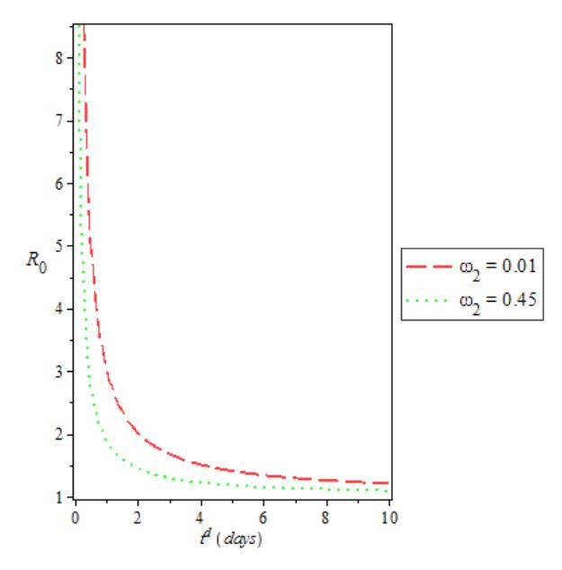
Figure 2: Impact of varying the rate of isolation rate, ω² on R⁰ against doubling time, t d .

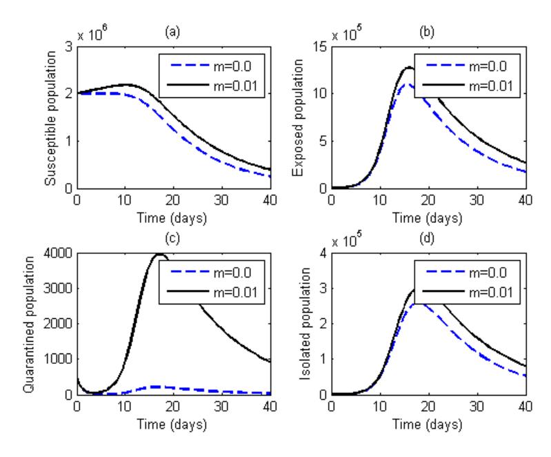
Figure 3: Impact of influx of exposed immigrants on (a) susceptible, (b) exposed individuals, (c) Quarantined and (d) Isolated population dynamics.

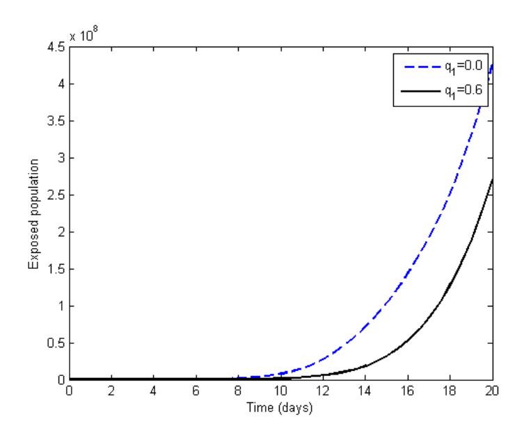
Figure 4: Impact of quarantine (q¹ = 0.6) at the point of entry on the exposed individuals.

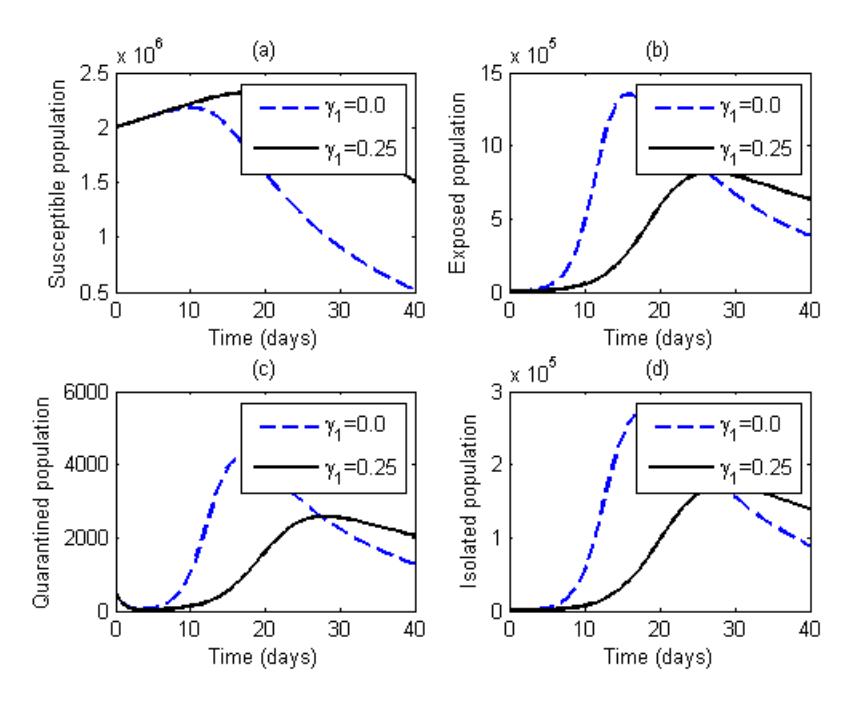
Figure 5: Impact of recovery rate due to body immune system on (a) susceptible, (b) exposed individuals, (c) Quarantined and (d) Isolated population dynamics.

5. CONCLUSION

In the study, a non-linear mathematical model is proposed and analyzed to study the transmission dynamics of COVID-19 in the presence of exposed immigrants. The model assumes strongly that any immigrant is suspected to be exposed to the virus and thus quarantined at the point of entry, and all symptomatic individuals of COVID-19 can not travel. By analyzing the model analytically, we computed a basic reproduction number, R0. We noted that when R⁰ < 1 (i.e. the product of transmission rate and number of contacts is less than the sum of natural death rate and recovery rate due to good body immune system) then the disease is eliminated. However, as long as exposed immigrants continue joining the population without being screened, the COVID-19-free equilibrium will always be unattainable, since the parameter m > 0 with immigrants force R⁰ > 1. When R⁰ > 1, COVID-19 becomes endemic and remain in the community. In addition, the system experiences transcritical bifurcation near the COVID-19-free equilibrium when R⁰ = 1. By simulation, it is shown that controlling the influx of exposed immigrants (by closing all borders through quarantine) will effectively reduce the number of exposed people who are infectious and placing immigration ban on immigrants during COVID-19 will limit the level of susceptibility of individuals in the community. The ban will also reduced the rate of infection of COVID-19 among the people. It is also revealed in the study that in the presence of isolation rate, the doubling time for COVID-19 gets longer and that slows the spread of the disease.

ACKNOWLEDGEMENT

The authors are thankful to the editor and anonymous reviewers for their careful reading, suggestions and useful comments that helped to improve the quality of the manuscript.