

1. INTRODUCTION
Malaria is one of the most infectious diseases in Sub-Saharan Africa and due to climatic dynamics in recent times, it continues to spread across other new places. Africa accounts for 94% of an estimated global cases of 229 million [1]. Malaria induced mortality is 409,000 for 2019 year alone [1]. The infected anopheles mosquitoes transmit the malaria parasites by biting human beings. The mosquitoes thrive on the moderate-towarm temperatures with high humidity and non-moving water bodies that are available for the vectors to lay their eggs [2]. The global warming phenomenon is one of the key drivers for the spread of malaria parasites across the continents. The quality of environmental management plays a major role in controlling the spread of the disease [3].
Poverty is characterized by the individuals inability to undertake so many humans activities. Man's inability to function properly due to poverty increases that possibility of being infected by diseases including malaria. Both material and human resources are needed to control malaria effectively in any community or society. The socio-economic conditions of a community or a country determines the quality of health facilities available for the people in accessing medical care [4], [3]. It is common in Africa to find a lot of individuals who have malaria parasites but cannot access health care because of their status or class in the society. The consequence is that these individuals may result to traditional treatment. This leads to drug resistance to the disease and other complications.
The effect of status or class on Sub-Saharan Africa cannot be ignored in this subject matter. Typically, individuals are either in the high or low status and this determines the quality of life the individual has in the society. Those in the lower status or class usually live in poor households where sanitary conditions are poor. This creates an environment that enhances the spread of malaria. In some extreme instances, those affected individuals are not able to access medical care because of poverty [2]. This sometimes leads to some complication such as lungs and kidneys related issues and eventually the individual may die. Persons who are of high ranked status and financially sound are mostly highly educated people. They live in good houses with standard environmental practices which minimizes the spread of the malaria.
The players in the health sector require reliable information in order to predict the future trend of epidemics such as malaria [3]. In recent times, mathematical modelling as an aspect of discipline in mathematics has been a valuable tool that provides qualitative information which leads to proper planning in many epidemic cases [2], [5], [6]. In the past century, many researchers have focused on developing different malaria models with deterministic approaches. The ultimate goal is to provide qualitative information that helps to reduce the spread of the disease.
In most recent times, fractional calculus has been noticed to be a formidable concept in mathematical modelling processes. The fractional derivative concepts hinge on both past and present data in order to predict the future [7], [8], [9]. This concept possesses memory effect which aids in accurate prediction. The Caputo operator is non-local and it obeys power law and cannot predict accurately in a complex phenomenon [7], [10]. Due to this shortcoming, a new operator called Caputo-Fabrizio was developed based on exponential law characterised by nonsingular kernel [11]. Even though this operator has a crossover property that makes it possible to stretch from one operator to another naturally, it is not every system in real life domain that follows exponential law. Atangana and Baleanu currently developed a robust operator that hinges on Mittag-Leffler function which is both non-local and non-singular [12], [13], [14], [15]. The operator has the ability to stretch from one operator to another leading to quality prediction in some complex systems.
Few years ago, Atangana and Araz [16] developed a stochastic version of all three basic operators as stated earlier. The stochastic aspect is to help account for the fluctuations in almost all real life applications of fractional calculus. In epidemics for example, disease cases including malaria are not the same everyday. Din et al., [17] examined dengue fever model utilising stochastic dynamics to account for the variations in the spread of the disease. Meksianis and Adi in [18], examined the impacts of individual awareness and vector controls on malaria dynamics based on multiple optimal control and found out that awareness in the presence of malaria infection was the best way of reducing the disease in the community. Suandi et al., [19] explored the dynamics of one-locus model and presented the evolutionary dynamics of resistance against insecticide in anopheles mosquitoes in the environment.
Alkahtani and Koca [20] investigated an SIR model using fractional stochastic to present the existence and uniqueness of solutions of the model. Alkinlar et al.,[21] constructed a mathematical model incorporating a white noise and obtained some useful numerical solutions. Omar et al., [22] studied a COVID model in the case of Egypt and obtained a conclusive evidence of the effect of the stochastic component on the spread of the COVID. Sweilam et al.,[23] developed a stochastic fraction order COVID model and examined the dynamics of the spread of the disease. Atangana and Araz [16] modelled COVID and presented a new numerical scheme in solving fractional stochastic models. They showed the existence and uniqueness of the COVID model solutions via stochastic approach.
The main aim of the fractional stochastic application to this work is to account for randomness and generalised Mittag-Leffler function behaviour in the malaria model. The operator employed for this study utilizes the crossover property which allows the tails of the kernel to extend beyond this Mittag-Leffler function (ML) to other operators. The fractional order stochastic model will provide more detailed information of the proposed model than the deterministic one, due to the crossover and random properties as stated earlier. Other studies buttress the point that stochastic simulation of a model is likely to provide information close to the actual data [24]. This paper therefore, utilises the Atangana and Araz nonlocal [16] and nonsingular operator with stochastic component to account for the fluctuations in the spread of malaria. The study would examine the existence and uniqueness of solutions of the malaria model.
2. MATHEMATICAL PRELIMINARIES
Definition 2.1. For a function \(u : [a, b] \to R\), the (left) Caputo fractional derivative of order p is expressed as:
\[{}_{a}^{C}D_{t}^{p}u(t) = \frac{1}{\Gamma(n-p)} \int_{a}^{t} u^{(n)}(\varpi)(t-\varpi)^{n-p-1} d\varpi, \qquad n-1
Similarly, the corresponding Caputo fractional integral is given by
\[{}_{a}^{C}I_{t}^{p}u(t) = \frac{1}{\Gamma(p)} \int_{a}^{t} u(\varpi)(t - \varpi)^{p-1} d\varpi.\] (2)
Definition 2.2. Let \(u \in A^1(a,b), b > a\), and 0 . Then, the newly developed fractional Atangana-Baleanu derivative in Caputo sense (AB) is expressed as:
\[{}_{a}^{AB}D_{t}^{p}u(t) = \frac{B(p)}{1-p} \int_{a}^{t} u'(\varpi)E_{P} \left[ -\frac{p}{1-p}(t-\varpi)^{p} \right] d\varpi, \tag{3}\] where AB(p) depicts the normalization function fulfilling AB(0) = AB(1) = 1 and \(E_p\) represents the Mittag-Leffler function
\[E_p(z) = \sum_{k=0}^{\infty} \frac{(z^p)^k}{\Gamma(pk+1)}, \qquad p > 0.\] (4)
The connected AB fractional integral is defined as:
\[{}_{a}^{AB}I_{t}^{p}u(t) = \frac{1-p}{B(p)}u(t) + \frac{p}{B(p)\Gamma(p)} \int_{a}^{t} u(\varpi)(t-\varpi)^{p-1}d\varpi.\] (5)
3. MODEL FORMULATION
This model fractionalised Olaniyi et al., [25] malaria status model in which the total population is partitioned into human population, \(Z_h(t)\) and vector population \(Z_v(t)\) respectively. Further, the total human population is subdivided into \(S_h(t)\) high status, susceptible high status humans, \(S_l(t)\) susceptible low status humans, \(I_h(t)\), infectious high status humans, \(I_h(t)\) infectious low status humans, \(R_h(t)\) recovered high status humans, \(R_l(t)\) recovered low status humans. Thus, \(Z_h = S_h(t) + S_l(t) + I_h(t) + I_l(t) + R_h(t) + R_l(t)\). The total vector population is partitioned into \(S_v(t)\) Susceptible mosquitoes and \(I_v(t)\) Infectious mosquitoes. Thus, \(Z_v(t) = S_v(t) + I_v(t)\). This operator is a non-local and non-singular which possesses a crossover property. In order to have same dimensions for both left and right hand, some parameters in the resultant fractional derivative model are modified. This leads to the following system of equations:
with the following initial condition
\[S_h(0) = S_{h0} \ge 0, S_l(0) = S_{l0} \ge 0, I_h(0) = I_{h0} \ge 0, I_l(0) = I_{l0} \ge 0,\] \[R_h(0) = R_{h0} \ge 0, R_l(0) = R_{l0} \ge 0, S_v(0) = S_{v0} \ge 0, I_v(0) = I_{v0} \ge 0\] (7)
The Table 1 shows the symbols and parameter description
Table 1: Parameters descriptions.
| Symbol | Parameter description |
|---|---|
| \(\omega\) | Fraction of high status humans' recruitment. |
| \(\Pi_h\) | Recruitment rate for humans. |
| a | Modification parameter for reduced transmission for humans. |
| \(\beta_l\) | Transmission rate of mosquitoes to humans. |
| \(\nu\) | Waning rates of high status acquired immunity. |
| \(\delta_l\) | Mobility rates of susceptible low status move into high status classes. |
| \(\mu_h\) | Natural mortality rates of humans. |
| \(\frac{\mu_h}{\delta_h}\) | Mobility rates of susceptible high status move into low status classes. |
| \(\sigma\) | Waning rates of low social acquired immunity. |
| \(\eta\) | Disease-induced mortality rates of high infectious humans. |
| \(\gamma\) | Recovery rates of low infectious individuals. |
| \(\Pi_v\) | Recruitment rate for mosquitoes. |
| \(\beta_v\) | Transmission rate of humans to mosquitoes. |
| \(\phi\) | Modification parameters for reduced transmission. |
| \(\mu_v\) | Mosquitoes natural mortality rate. |
4. MODEL ANALYSIS
4.1. Non-negative solution of the Model
Theorem 4.1. The solution of the malaria model (6) in the fractional order derivative of a AB operator with initial condition (7) singular and bound in \(R^8_{\perp}\).
Proof: The existence and uniqueness of the malaria model (6) on the given initial \((0, \infty)\) can be derived following the process as in the work of Muhammad et al., [26]. The positively invariant region of the malaria model (6) can be established as;
\[\begin{array}{lll} {}_{0}^{AB}D_{t}^{p}S_{h}|_{S_{h=0}} & = & \varpi^{p}\Pi_{h}^{p} + \nu^{p}R_{h} - \delta_{l}^{p}S_{l} \geq 0, \\ {}_{0}^{AB}D_{t}^{p}S_{l}|_{S_{l=0}} & = & (1 - \varpi^{p})\Pi_{h}^{p} + \sigma^{p}R_{l} - \delta_{h}^{p}S_{h} \geq 0, \\ {}_{0}^{AB}D_{t}^{p}I_{h}|_{I_{h=0}} & = & a^{p}\beta_{l}^{p}S_{h}I_{v} \geq 0, \\ {}_{0}^{AB}D_{t}^{p}I_{l}|_{I_{l=0}} & = & \beta_{l}^{p}S_{l}I_{v} \geq 0, \\ {}_{0}^{AB}D_{t}^{p}R_{l}|_{R_{l=0}} & = & \sigma^{p}I_{h} \geq 0, \\ {}_{0}^{AB}D_{t}^{p}R_{l}|_{R_{l=0}} & = & \gamma^{p}I_{l} \geq 0, \\ {}_{0}^{AB}D_{t}^{p}S_{v}|_{S_{v=0}} & = & \Pi_{v}^{p} \geq 0, \\ {}_{0}^{AB}D_{t}^{p}I_{v}|_{I_{v=0}} & = & \beta_{v}^{p}\left(I_{l} + \phi^{p}I_{h}\right)S_{v} \geq 0. \end{array} \tag{8}\]
If we have \((S_h(0),S_l(0),I_h(0),I_l(0),R_h(0),R_l(0),S_v(0),I_v(0))\in R^8_\alpha\), the solution of the model 6 \((S_h(t),S_l(t),I_h(t),I_l(t),R_h(t),R_l(t),S_v(t),I_v(t))\) cannot outflow from the hyperplanes \(S_h=0,S_l=0,I_h=0,I_l=0,R_h=0,R_l=0,S_v=0\), and \(I_v(0)\). The hyperplane points towards the non-negative orthant \(R^8_+\) and therefore, positively invariant set. This is the end of the proof of the Theorem 1.
Lemma 4.2. The closed set
\[\Phi_1 = \left\{ (S_h(t), S_l(t), I_h(t), I_l(t), R_h(t), R_l(t) : Z_h(t)) \in R_+^6 : Z_h(t) \le \frac{\Pi_h^p}{\mu_h^p} \right\},\,\] and
\[\Phi_2 = \left\{ (S_v(t), I_v(t)) \in R_+^2 : Z_h(t) \le \frac{\Pi_v^p}{\mu_v^p} \right\}.\]
It is considered positively invariant with regard to malaria status model (6).
Proof: The total human and vector populations in model (6), with respect to Atangana-Baleanu is given by:
\[{}_{0}^{AB}D_{t}^{p}Z_{h} = \Pi_{h}^{p} - \mu_{h}^{p}Z_{h}(t) \le \Pi_{h}^{p} - \mu_{h}^{p}Z_{h}(t),\] and \[{}_{0}^{AB}D_{t}^{p}Z_{v} = \Pi_{v}^{p} - \mu_{v}^{p}Z_{v}(t) \le \Pi_{v}^{p} - \mu_{v}^{p}Z_{v}(t),\] (9)
Utilizing the concept of Laplace Transform, the equation (9) is organised as:
\[Z_{h}(t) \leq \left(\frac{B(p)}{B(p) + (1-p)\mu_{h}^{p}} Z_{h}(0) + \frac{(1-p)\Pi_{h}^{p}}{B(p) + (1-p)\mu_{h}^{p}}\right) E_{p,1}(-\beta t^{p})\] \[+ \frac{\Pi_{h}^{p}(p)}{AB(p) + (1-p)\mu_{h}^{p}} E_{p,p+1}(-\beta_{0}t^{p}),\] \[Z_{v}(t) \leq \left(\frac{B(p)}{B(p) + (1-p)\mu_{v}^{p}} Z_{v}(0) + \frac{(1-p)\Pi_{v}^{p}}{B(p) + (1-p)\mu_{v}^{p}}\right) E_{p,1}(-\beta t^{p})\] \[+ \frac{\Pi_{v}^{p}(p)}{B(p) + (1-p)\mu_{v}^{p}} E_{p,p+1}(-\beta_{1}t^{p}),\] \[(10)\] where \(\beta_0 = \frac{\mu_h^p p}{B(p) + (1-p)\mu_h^p}\), \(\beta_1 = \frac{\mu_v^p p}{B(p) + (1-p)\mu_v^p}\) and \(E_{p,\beta_i}\) constitutes the two Mittag-Leffler(ML) function parameters. Considering the fact that ML function has an asymptotic characteristic and given by:
\[E_{p_1,p_2}(\varpi) \approx -\sum_{k}^{\lambda} \frac{\varpi^{-k}}{T(p_2 - p_1 k)} + o\left(|\varpi|^{-1 - \chi}\right) \left(|\varpi| \to \infty, \frac{p_1 \pi}{2} < |\arg(\varpi)| \le \pi\right), \tag{11}\]
it is recognizable to appreciate that \(Z_h \leq \frac{\Pi_h^p}{\mu_h^p}\) and \(Z_v \leq \frac{\Pi_v^p}{\mu_v^p}\) as \(t \to \infty\) respectively. Hence, the complete solutions of the malaria status class model (6), initial conditions which are in \(\Phi_1\) and \(\Phi_2\) respectively remain in \(\Phi_1\) and \(\Phi_2\) whenever t>0. Therefore, \(\Phi_1\) and \(\Phi_2\) are considered positively invariant in the region with regard to system (6).
4.2. Existence and Uniqueness of the Solution with AB operator
This section examines the existence and uniqueness of the solution connected with ML function malaria status model (6). To begin with, the system equation model (6) is reorganised we as:
\[\begin{cases} A^{B} D_{t}^{p} u(t) = J(u(t)), & 0 < t < T < \infty, \\ u(0) = u_{0}, & \end{cases}\] (12)
where u represents the state vector expressed as \(u = (S_h, S_l, I_h, I_l, R_h, R_l, S_v, I_v)\), J depicts an actual-valued continuous vector function given by:
\[J = \begin{pmatrix} J_1 \\ J_2 \\ J_3 \\ J_4 \\ J_5 \\ J_6 \\ J_7 \\ J_8 \end{pmatrix} = \begin{pmatrix} \omega^p \Pi_h^p - a^p \beta_l^p S_h I_v + \nu^p R_h + \delta_l^p S_l - (\mu_h^p + \delta_h^p) S_h, \\ (1 - \omega^p) \Pi_h^p - \beta_l^p S_l I_v + \sigma^p R_l + \delta_h^p S_h - (\mu_h^p + \delta_l^p) S_l, \\ a^p \beta_l^p S_h I_v - (\mu_h^p + \theta^p + \eta^p) I_h, \\ \beta_l^p S_l I_v - (\mu_h^p + \gamma^p) I_l, \\ \theta^p I_h - (\mu_h^p + \nu^p) R_h, \\ \gamma^p I_l - (\mu_h^p + \sigma^p) R_l, \\ \Pi_v^p - \beta_v^p (I_l + \phi^p I_h) S_v - \mu_v^p S_v, \\ \beta_v^p (I_l + \phi^p I_h) S_v - \mu_v^p I_v. \end{pmatrix}\] \[(13)\] and \(u_0\) stands for the initial state vector used in the malaria model (6). By the fact that J constitutes a quadratic vector function, it accomplishes the Lipschitz condition. Hence, there exist a constant Q in a manner that
\[||J(u(t)) - J(v(t))|| \le Q ||u(t) - v(t)||.\] (14)
It is interesting to note that the existence and uniqueness of solutions models using AB operator has been investigated by several authors[13], [14]. The following theorem will be used theoretically to examine the existence and uniqueness of solution of the malaria status model with ML function.
Theorem 4.3. (Existence and uniqueness). The fractional-order derivative malaria status model (12) possesses a distinctive solution whenever the following condition exists:
\[\frac{1-p}{AB(p)}Q + \frac{p}{AB(p)\Gamma(p)}Q\Gamma^p < 1. \tag{15}\]
Proof: Making use of the AB fractional integral operator (5), the following is obtained:
\[u(t) = u_0 + \frac{1-p}{AB(p)}J(u(t)) + \frac{p}{AB(p)\Gamma(p)} \int_0^t (t-\varpi)^{p-1}J(u(\varpi))d\varpi.\] (16)
It is assumed that F = (0,T) and \(G : E(G,R^8) \to E(G,R^8)\) operator is defined as:
\[J(u(t)) = u_0 + \frac{1-p}{AB(p)}J(u(t)) + \frac{p}{AB(p)\Gamma(p)} \int_0^t (t-\varpi)^{p-1}J(u(\varpi))d\varpi.\] (17)
The equation (16) is arranged as follows:
\[u(t) = J(u(t)). (18)\]
Let \(\|.\|_G\) symbolise the supremum norm on G, i.e.,
\[||u(t)||_G = \sup_{t \in G} ||u(t)||, \qquad u(t) \in E(G, R^8).\] (19)
Then \(E(G, \mathbb{R}^8)\) with \(\|.\|_G\) represents, a Banach space. Furthermore, it is simply demonstrated that
\[\left\| \int_{0}^{t} K(t, \varpi) u(\varpi) d\varpi \right\|_{G} \le T \left\| K(t, \varpi) \right\|_{G} \left\| u(t) \right\|_{G,} \tag{20}\]
where \(u(t) \in E(G, \mathbb{R}^8), K(t, \varpi) \in E(G^2, \mathbb{R})\) and
\[||K(t,\varpi)||_G, \sup_{t,\varpi\in G} |K(t,\varpi), \quad |K(t,\varpi)\in E(G^2,R).\] (21)
Making use of the definition of operator J given in equation (17), and in addition to equations (14) and (20), the following is arrived at:
\[||J(u(t)) - J(v(t))||_{G} \leq \frac{1-p}{AB(p)} ||J(u(t)) - J(v(t))||_{G} + \frac{p}{AB(p)\Gamma(p)} T^{p} ||G(u(\varpi)) - G(v(\varpi))||_{G}\] \[\leq \left(\frac{1-p}{AB(p)} Q + \frac{p}{AB(p)\Gamma(p)} Q T^{p}\right) ||u(t) - J(v(t))||_{G}.\] (22)
Thus, one obtains
\[\|J(u(t)) - J(v(t))\|_{G} \le Q \|u(t) - v(t)\|_{G}, \tag{23}\] where \(L = \frac{1-p}{AB(p)}Q + \frac{p}{AB(p)\Gamma(p)}QT^p\). If condition (15) is fulfilled, the operator J will be considered to be contraction on \(E(G^2,R)\). Hence, as a result of Banach fixed point theorem, model system (12) possesses a distinctive solution.
4.3. Existence and Uniqueness of Solutions with Stochastic Component
In this section, the existence and uniqueness solution of malaria status model with the stochastic component (24) is examined. Diseases such as malaria has dynamics very difficult to predict in a deterministic manner. The infection rate can change any time and therefore the fluctuation as an aspect ought be accounted for in modelling malaria transmission. It is against this principle that model is examined with a stochastic component. The equation is therefore reformulated to include the stochastic compartment as follows:
\[\begin{array}{lll} ^{AB}D_{t}^{p}S_{h}(t) & = & (\omega^{p}\Pi_{h}^{p} - a^{p}\beta_{l}^{p}S_{h}I_{v} + \nu^{p}R_{h} + \delta_{l}^{p}S_{l} - (\mu_{h}^{p} + \delta_{h}^{p})S_{h}) dt + b_{1}S_{h}(t)dF_{1}(t), \\ ^{AB}D_{t}^{p}S_{l}(t) & = & ((1 - \omega^{p})\Pi_{h}^{p} - \beta_{l}^{p}S_{l}I_{v} + \sigma^{p}R_{l} + \delta_{h}^{p}S_{h} - (\mu_{h}^{p} + \delta_{l}^{p})S_{l}) dt + b_{2}S_{l}(t)dF_{2}(t), \\ ^{AB}D_{t}^{p}I_{h}(t) & = & (a^{p}\beta_{l}^{p}S_{h}I_{v} - (\mu_{h}^{p} + \theta^{p} + \eta^{p})I_{h}) dt + b_{3}I_{h}(t)dF_{3}(t), \\ ^{AB}D_{t}^{p}I_{l}(t) & = & (\beta_{l}^{p}S_{l}I_{v} - (\mu_{h}^{p} + \gamma^{p})I_{l}) dt + b_{4}I_{l}(t)dF_{4}(t), \\ ^{AB}D_{t}^{p}R_{h}(t) & = & (\theta^{p}I_{h} - (\mu_{h}^{p} + \nu^{p})R_{h}) dt + b_{5}R_{h}(t)dF_{5}(t), \\ ^{AB}D_{t}^{p}R_{l}(t) & = & (\gamma^{p}I_{l} - (\mu_{h}^{p} + \sigma^{p})R_{l}) dt + b_{6}R_{l}(t)dF_{6}(t), \\ ^{AB}D_{t}^{p}S_{v}(t) & = & (\Pi_{v}^{p} - \beta_{v}^{p}(I_{l} + \phi^{p}I_{h})S_{v} - \mu_{v}^{p}S_{v}) dt + b_{7}S_{v}(t)dF_{7}(t), \\ ^{AB}D_{t}^{p}I_{v}(t) & = & (\beta_{v}^{p}(I_{l} + \phi^{p}I_{h})S_{v} - \mu_{v}^{p}I_{v}) dt + b_{8}I_{v}(t)dF_{8}(t). \end{array} \tag{25}\]
where \(F_i(t)\), i = 1, 2, 3, 4, 5, 6, 7, 8 depicts the standard Brownian motion and \(b_i = 1, 2, 3, 4, 5, 6, 7, 8\) is the stochastic constants.
Theorem 4.4. Let consider that there exist a certain positive constants q, \(\overline{q}\) such that:
(i) \[\forall \in \{1, ..., 8\}\]
\[|J(u,t) - J(u',t)|^2 \le q|u - u'|.\]
(ii) \[\forall (u,t) \in R \times [0,T]\] \[|J(u,t)|^2 \leq \overline{q}(1+|u|^2).\]
Proof: The proof begins by examining the function J1(t, Sh, Sl , Ih, Il , Rh, Rl , Sv, Iv). In this regard, the first condition is worked out as follows:
\[\begin{split} |J_{1}(S_{h},t)-J_{1}(S_{h}^{*},t)|^{2} &= |-a^{p}\beta_{l}^{p}I_{v}(S_{h}-S_{h}^{*})-(\mu_{h}^{p}+\delta_{h}^{p})(S_{h}-S_{h}^{*})|^{2} \\ &= |-(a^{p}\beta_{l}^{p}I_{v}+(\mu_{h}^{p}+\delta_{h}^{p}))(S_{h}-S_{h}^{*})|^{2}, \\ &\leq \left\{2(a^{p})^{2}(\beta_{l}^{p})^{2}|I_{v}|^{2}+2(\mu_{h}^{p}+\delta_{h}^{p})^{2}\right\}|S_{h}-S_{h}^{*}|^{2}, \\ &\leq \left\{2(a^{p})^{2}(\beta_{l}^{p})^{2}|S_{up}|I_{v}|^{2}+2(\mu_{h}^{p}+\delta_{h}^{p})^{2}\right\}|S_{h}-S_{h}^{*}|^{2}, \\ &\leq \left\{2(a^{p})^{2}(\beta_{l}^{p})^{2}||I_{v}||_{\infty}^{2}+2(\mu_{h}^{p}+\delta_{h}^{p})^{2}\right\}|S_{h}-S_{h}^{*}|^{2}, \\ &\leq \left\{2(a^{p})^{2}(\beta_{l}^{p})^{2}||I_{v}||_{\infty}^{2}+2(\mu_{h}^{p}+\delta_{h}^{p})^{2}\right\}|S_{h}-S_{h}^{*}|^{2}, \\ &\leq q_{1}|S_{h}-S_{h}^{*}|^{2}. \\ &|J_{2}(S_{l},t)-J_{2}(S_{l}^{*},t)|^{2} &= |-\beta_{l}^{p}I_{v}(S_{l}-S_{l}^{*})-(\mu_{h}^{p}+\delta_{l}^{p})(S_{l}-S_{l}^{*})|^{2}, \\ &\leq \left\{2(\beta_{l}^{p})^{2}I_{v}|^{2}+2(\mu_{h}^{p}+\delta_{l}^{p})^{2}\right\}|S_{l}-S_{l}^{*}|^{2}, \\ &\leq \left\{2(\beta_{l}^{p})^{2}S_{up}|I_{v}|^{2}+2(\mu_{h}^{p}+\delta_{l}^{p})^{2}\right\}|S_{l}-S_{l}^{*}|^{2}, \\ &\leq \left\{2(\beta_{l}^{p})^{2}||I_{v}||_{\infty}^{2}+2(\mu_{h}^{p}+\delta_{l}^{p})^{2}\right\}|S_{l}-S_{l}^{*}|^{2}, \\ &\leq q_{2}|S_{l}-S_{l}^{*}|^{2}. \\ &|J_{3}(I_{h},t)-J_{3}(I_{h}^{*},t)|^{2} &= |-(\mu_{h}^{p}+\theta^{p}+\eta^{p})(I_{h}-I_{h}^{*})|^{2}, \\ &\leq ((\mu_{h}^{p}+\theta^{p}+\eta^{p})^{2}|(I_{h}-I_{h}^{*})|^{2}, \\ &\leq q_{3}|I_{h}-I_{h}^{*}|^{2}. \end{aligned}\]
\[|J_{4}(I_{l},t) - J_{4}(I_{l}^{*},t)|^{2} = |-(\mu_{h}^{p} + \gamma^{p})(I_{l} - I_{l}^{*})|^{2},\] \[\leq (\mu_{h}^{p} + \gamma^{p})^{2} |(I_{l} - I_{l}^{*})|^{2},\] \[\leq ((\mu_{h}^{p} + \gamma^{p})^{2} + l_{2}) |(I_{h} - I_{h}^{*})|^{2},\] \[\leq q_{4} |I_{h} - I_{h}^{*}|^{2}.\] (28)
\[|J_{5}(R_{h},t) - J_{5}(R_{h}^{*},t)|^{2} = |-(\mu_{h}^{p} + \nu^{p})(R_{h} - R_{h}^{*})|^{2},\] \[\leq (\mu_{h}^{p} + \nu^{p})^{2} |(R_{h} - R_{h}^{*})|^{2},\] \[\leq ((\mu_{h}^{p} + \nu^{p})^{2} + l_{3}) |(R_{h} - R_{h}^{*})|^{2},\] \[\leq q_{5} |R_{h} - R_{h}^{*}|^{2}.\] \[(29)\]
\[|J_{6}(R_{l},t) - J_{6}(R_{l}^{*},t)|^{2} = |-(u_{h}^{p} + \sigma^{p})(R_{l} - R_{l}^{*})|^{2},\] \[\leq (\mu_{h}^{p} + \sigma^{p})^{2} |(R_{l} - R_{l}^{*})|^{2},\] \[\leq ((\mu_{h}^{p} + \sigma^{p})^{2} + l_{4}) |(R_{l} - R_{l}^{*})|^{2},\] \[\leq q_{6} |R_{l} - R_{l}^{*}|^{2}.\] (30)
\[|J_{7}(S_{v},t) - J_{7}(S_{v}^{*},t)|^{2} = |-\beta_{v}^{p}(I_{l} + \phi^{p}I_{h})(S_{v} - S_{v}^{*}) - \mu_{v}^{p}(S_{v} - S_{v}^{*})|^{2},\] \[= |-(\beta_{v}^{p}I_{l} + \beta_{v}^{p}\phi^{p}I_{h} + \mu_{v}^{p})(S_{v} - S_{v}^{*})|^{2},\] \[\leq \left\{3(\beta_{v}^{p})^{2} |I_{1}|^{2} + 3(\beta_{v}^{p})^{2}(\phi^{p})^{2} |I_{h}|^{2} + 3(\mu_{v}^{p})^{2}\right\} |S_{v} - S_{v}^{*}|^{2}, \qquad (31)\] \[\leq \left\{3(\beta_{v}^{p})^{2} \sup_{0 \leq t \leq T} |I_{l}|^{2} + 3(\beta_{v}^{p})^{2}(\phi^{p})^{2} \sup_{0 \leq t \leq T} |I_{h}|^{2} + 3(\mu_{v}^{p})^{2}\right\} |S_{v} - S_{v}^{*}|^{2},\] \[\leq \left\{3(\beta_{v}^{p})^{2} ||I_{l}||_{\infty}^{2} + 3(\beta_{v}^{p})^{2}(\phi^{p})^{2} ||I_{h}||_{\infty}^{2} + 3(\mu_{v}^{p})^{2}\right\} |S_{l} - S_{l}^{*}|^{2},\] \[\leq q_{7} |S_{v} - S_{v}^{*}|^{2}.\] \[|J_{8}(I_{v}, t) - J_{8}(I_{v}^{*}, t)|^{2} = |-(\mu_{v}^{p})(I_{v} - I_{v}^{*})|^{2},\] \[\leq ((\mu_{v}^{p})^{2} + l_{5})^{2} |I_{v} - I_{v}^{*}|^{2},\] \[\leq q_{8} |I_{v} - I_{v}^{*}|^{2}.\] \[(32)\]
The second condition is examined as follows:
\[\text{[rumus tidak dapat ditampilkan dengan baik — lihat PDF asli]}\] with respect to the condition \(\frac{(a^p)^2(\beta_l^p)^2 ||I_v||_{\infty}^2 + ((\mu_h^p)^2 + (\delta_h^p)^2)^2}{(\omega^p)^2(\Pi_h^p)^2 + (\nu^p)^2 ||R_h||_{\infty}^2 + (\delta_l^p)^2 ||S_l||_{\infty}^2} < 1.\)
\[\begin{split} |J_{2}(S_{l},t)|^{2} &= \left| (1-\omega^{p}) \Pi_{h}^{p} - \beta_{l}^{p} S_{l} I_{v} + \sigma^{p} R_{l} + \delta_{h}^{p} S_{h} - (u_{h}^{p} + \delta_{l}^{2} p) S_{l} \right|^{2}, \\ &\leq \left( 5(1-\omega^{p})^{2} (\Pi_{h}^{p})^{2} + 5(\beta_{l}^{p})^{2} |S_{l}|^{2} |I_{v}|^{2} + 5(\sigma^{p})^{2} |R_{l}|^{2} + 5(\delta_{h}^{p})^{2} |S_{h}|^{2} + 5((u_{h}^{p})^{2} + (\delta_{l}^{p})^{2})^{2} |S_{l}|^{2} \right), \\ &\leq 5(1-\omega^{p})^{2} (\Pi_{h}^{p})^{2} + 5(\beta_{l}^{p})^{2} |S_{l}|^{2} \sup_{0 \leq t \leq T} |I_{v}|^{2} + 5(\sigma^{p})^{2} \sup_{0 \leq t \leq T} |R_{l}|^{2} + 5(\delta_{h}^{p})^{2} \sup_{0 \leq t \leq T} |S_{h}|^{2} + 5((\mu_{h}^{p})^{2} + 6(h_{l}^{p})^{2})^{2} |S_{l}|^{2}, \\ &\leq 5(1-(\omega^{p})^{2})^{2} (\Pi_{h}^{p})^{2} + 5(\beta_{l}^{p})^{2} |S_{l}|^{2} |I_{v}||_{\infty}^{2} + 5(\sigma^{p})^{2} ||R_{l}||_{\infty}^{2} + 5(\delta_{h}^{p})^{2} ||S_{h}||_{\infty}^{2} + 5((\mu_{h}^{p})^{2} + 5(\delta_{l}^{p})^{2})^{2} |S_{l}|^{2}, \\ &\leq 5\left( (1-\omega^{p})^{2} (\Pi_{h}^{p})^{2} + (\sigma^{p})^{2} ||R_{l}||_{\infty}^{2} + (\delta_{h}^{p})^{2} ||S_{h}||_{\infty}^{2} \right) \times \\ &\left( 1 + \frac{(\beta_{l}^{p})^{2}}{(1-(\omega^{p})^{2})^{2} (\pi_{h}^{p})^{2} + (\sigma^{p})^{2} ||R_{l}||_{\infty}^{2} + (\delta_{h}^{p})^{2} ||S_{h}||_{\infty}^{2}} \right) |S_{l}|^{2}, \\ &\leq \overline{q}_{2} \left( 1 + |S_{l}|^{2} \right). \end{split}\]
such that \[\frac{(\beta_l^p)^2 ||I_v||_{\infty}^2 + ((\mu_h^p)^2 + (\delta_l^p)^2)^2}{(1 - (\omega^p)^2)^2 (\Pi_h^p)^2 + (\sigma^p)^2 ||R_l||_{\infty}^2 + (\delta_h^p)^2 ||S_h||_{\infty}^2)} < 1.\] \[|J_3(I_h, t)|^2 = |(a^p \beta_l^p S_h I_v - (\mu_h^p + \theta^p + \eta^p) I_h|^2,\] \[\leq (2(\alpha^p)^2 (\beta_l^p)^2 |S_h|^2 |I_v|^2) + 2((\mu_h^p)^2 + (\theta^p)^2 + (\eta^p)^2)^2 |I_h|^2),\] \[(35)\]
\[\leq \left(2(\alpha^{p})^{2}(\beta_{l}^{p})^{2}|S_{h}|^{2}|I_{v}|^{2}\right) + 2((\mu_{h}^{p})^{2} + (\theta^{p})^{2} + (\eta^{p})^{2})^{2}|I_{h}|^{2}),\] \[\leq 2\left((a^{p})^{2}(\beta_{l}^{p})^{2} \sup_{0 \leq t \leq T}|S_{h}|^{2} \sup_{0 \leq t \leq T}|I_{v}|^{2} + ((\mu_{h}^{p})^{2} + (\theta^{p})^{2} + (\eta^{p})^{2})^{2}|I_{h}|^{2}\right),\] \[\leq 2\left((a^{p})^{2}(\beta_{l}^{p})^{2}||S_{h}||_{\infty}^{2}||I_{v}||_{\infty}^{2} + (\mu_{h}^{p} + \theta^{p} + \eta^{p})^{2}|I_{h}|^{2}\right),\] \[\leq 2\left((a^{p})^{2}(\beta_{l}^{p})^{2}||S_{h}||_{\infty}^{2}||I_{v}||_{\infty}^{2}\right)\left(1 + \frac{(\mu_{h}^{p} + \theta^{p} + \eta^{p})^{2}}{(\alpha^{p})^{2}(\beta_{l}^{p})^{2}||S_{h}||_{\infty}^{2}||I_{v}||_{\infty}^{2}}|I_{h}|^{2}\right),\] \[\leq \overline{q}_{3}\left(1 + |I_{h}|^{2}\right).\] (36)
\(\text{in line with the condition} \quad \frac{(\mu_h^p + \theta^p + \eta^p)^2}{(a^p)^2 (\beta_l^p)^2 \ ||S_h||_\infty^2 \ ||I_v||_\infty^2} < 1.\)
\[|J_{4}(I_{l},t)|^{2} = |(\beta_{l}^{p}S_{l}I_{v} - (\mu_{h}^{p} + \gamma^{p})I_{l}|^{2},\] \[\leq (2(\beta_{l}^{p})^{2}|S_{l}|^{2}|I_{v}|^{2}) + 2(\mu_{h}^{p} + \gamma^{p})^{2}|I_{l}|^{2}),\] \[\leq 2\left((\beta_{l}^{p})^{2} \sup_{0 \leq t \leq T} |S_{l}|^{2} \sup_{0 \leq t \leq T} |I_{v}|^{2} + (\mu_{h}^{p} + \gamma^{p})^{2}|I_{l}|^{2}\right),\] \[\leq 2\left((\beta_{l}^{p})^{2} ||S_{l}||_{\infty}^{2} ||I_{v}||_{\infty}^{2} + (\mu_{h}^{p} + \theta^{p} + \eta^{p})^{2}|I_{l}|^{2}\right),\] \[\leq 2\left((\beta_{l}^{p})^{2} ||S_{l}||_{\infty}^{2} ||I_{v}||_{\infty}^{2}\right) \left(1 + \frac{(\mu_{h}^{p} + \gamma^{p})^{2}}{(\beta_{l}^{p})^{2} ||S_{l}||_{\infty}^{2} ||I_{v}||_{\infty}^{2}}|I_{l}|^{2}\right),\] \[\leq \overline{q}_{4}\left(1 + |I_{l}|^{2}\right).\] \[(37)\] in the condition that \(\frac{(\mu_h^p+\gamma^p)^2}{(\beta_l^p)^2\;||S_l||_\infty^2\;||I_v||_\infty^2}<1.\)
\[|J_{5}(R_{h},t)|^{2} = |(\theta^{p}I_{h} - (\mu_{h}^{p} + \nu^{p})R_{h}|^{2},\] \[\leq (2(\theta^{p})^{2}|I_{h}|^{2} + 2(\mu_{h}^{p} + \nu^{p})^{2}|R_{h}|^{2}),\] \[\leq 2\left((\theta^{p})^{2} \sup_{0 \leq t \leq T} |I_{h}|^{2} + (\mu_{h}^{p} + \nu^{p})^{2}|R_{h}|^{2}\right),\] \[\leq 2\left((\theta^{p})^{2} ||I_{h}||_{\infty}^{2} + (\mu_{h}^{p} + \nu^{p})^{2}|R_{h}|^{2}\right),\] \[\leq 2\left((\theta^{p})^{2} ||I_{h}||_{\infty}^{2}\right) \left(1 + \frac{(\mu_{h}^{p} + \nu^{p})^{2}}{(\theta^{p})^{2} ||I_{h}||_{\infty}^{2}}|R_{h}|^{2}\right),\] \[\leq \overline{q}_{5}\left(1 + |I_{h}|^{2}\right).\] (38)
in the condition that \(\frac{(\mu_h^p + \nu^p)^2}{(\theta^p)^2 ||I_h||_{\infty}^2} < 1.\)
\[|J_{6}(R_{l},t)|^{2} = |(\gamma I_{l}^{p} - (\mu_{h}^{p} + \sigma^{p})R_{l}|^{2},\] \[\leq (2(\gamma^{p})^{2}|I_{l}|^{2} + 2(\mu_{h}^{p} + \sigma^{p})^{2}|R_{l}|^{2}),\] \[\leq 2\left((\gamma^{p})^{2} \sup_{0 \leq t \leq T} |I_{l}|^{2} + (\mu_{h}^{p} + \sigma^{p})^{2}|R_{l}|^{2}\right),\] \[\leq 2\left((\gamma^{p})^{2} ||I_{l}||_{\infty}^{2} + (\mu_{h}^{p} + \sigma^{p})^{2}|R_{l}|^{2}\right),\] \[\leq 2\left((\gamma^{p})^{2} ||I_{l}||_{\infty}^{2}\right) + \left(1 + \frac{(\mu_{h}^{p} + \sigma^{p})^{2}}{(\gamma^{p})^{2} ||I_{l}||_{\infty}^{2}}\right),\] \[\leq \overline{q}_{6}\left(1 + |I_{l}|^{2}\right).\] (39)
\(\text{such that} \quad \frac{(\mu_h^p + \sigma^p)^2}{(\gamma^p)^2 \; ||I_l||_{\infty}^2} < 1.\)
\[|J_{7}(S_{v},t)|^{2} = |\Pi_{v}^{p} - \beta_{v}^{p}(I_{l} + \phi^{p}I_{h})S_{v} - \mu_{v}^{p}S_{v}|^{2},\] \[\leq (4(\Pi_{v}^{p})^{2} + 4(\beta_{v}^{p})^{2}|I_{l}|^{2}|S_{v}|^{2} + 4(\phi^{p})^{2}(\beta_{v}^{p})^{2}|I_{h}|^{2}|S_{v}|^{2} + (\mu_{v}^{p})^{2}|S_{v}|^{2}),\] \[\leq 4\left((\Pi_{v}^{p})^{2} + (\beta_{v}^{p})^{2} \sup_{0 \leq t \leq T} |I_{l}|^{2}|S_{v}|^{2} + (\phi^{p})^{2}(\beta_{v}^{p})^{2} \sup_{0 \leq t \leq T} |I_{h}|^{2}|S_{v}|^{2} + (\mu_{v}^{p})^{2}|S_{v}|^{2}\right),\] \[\leq 4\left((\Pi_{v}^{p})^{2} + (\beta_{v}^{p})^{2}||I_{l}||_{\infty}^{2}|S_{v}|^{2} + (\phi^{p})^{2}(\beta_{v}^{p})^{2}||I_{h}||_{\infty}^{2}|S_{v}|^{2} + (\mu_{v}^{p})^{2}|S_{v}|^{2}\right),\] \[\text{[rumus tidak dapat ditampilkan dengan baik — lihat PDF asli]}\] \[\leq \overline{q}_{7}\left(1 + |S_{v}|^{2}\right).\] \[(40)\] in a manner that \(\frac{(\beta_v^p)^2 \ ||I_l||_\infty^2 + (\phi^p)^2 (\beta_v^p)^2 ||I_h||_\infty^2 + (\mu_v^p)^2}{(\Pi_v^p)^2} < 1.\)
\[\begin{split} \left|J_{8}(I_{v},t)\right|^{2} &= \left|\beta_{v}^{p}(I_{l}+\phi^{p}I_{h})S_{v}-\mu_{v}^{p}I_{v}\right|^{2}, \\ &\leq \left(3(\beta_{v}^{p})^{2}|I_{l}|^{2}|S_{v}|^{2}+3(\beta_{v}^{p})^{2}(\phi^{p})^{2}|I_{h}|^{2}|S_{v}|^{2}+(\mu_{v}^{p})^{2}|I_{v}|^{2}\right), \\ &\leq 3\left((\beta_{v}^{p})^{2}\sup_{0\leq t\leq T}|I_{l}|^{2}\sup_{0\leq t\leq T}|S_{v}|^{2}+(\beta_{v}^{p})^{2}(\phi^{p})^{2}\sup_{0\leq t\leq T}|I_{h}|^{2}\sup_{0\leq t\leq T}|S_{v}|^{2}+(\mu_{v}^{p})^{2}|I_{v}|^{2}\right), \\ &\leq 3\left((\beta_{v}^{p})^{2}||I_{l}||_{\infty}^{2}||S_{v}||_{\infty}^{2}+(\beta_{v}^{p})^{2}(\phi^{p})^{2}||I_{h}||_{\infty}^{2}||S_{v}||_{\infty}^{2}+(\mu_{v}^{p})^{2}|I_{v}|^{2}\right), \end{split}\]
\[\leq 3 \left( (\beta_{v}^{p})^{2} ||I_{l}||_{\infty}^{2} ||S_{v}||_{\infty}^{2} + (\beta_{v}^{p})^{2} (\phi^{p})^{2} ||I_{h}||_{\infty}^{2} ||S_{v}||_{\infty}^{2} \right) \times\] \[\left( 1 + \frac{(\mu_{v}^{p})^{2}}{(\beta_{v}^{p})^{2} ||I_{l}||_{\infty}^{2} ||S_{v}||_{\infty}^{2} + (\beta_{v}^{p})^{2} (\phi^{p})^{2} ||I_{h}||_{\infty}^{2} ||S_{v}||_{\infty}^{2}} |I_{v}|^{2} \right),\] \[\leq 3 \left( (\beta_{v}^{p})^{2} ||I_{l}||_{\infty}^{2} ||S_{v}||_{\infty}^{2} + (\beta_{v}^{p})^{2} (\phi^{p})^{2} ||I_{h}||_{\infty}^{2} ||S_{v}||_{\infty}^{2} \right) \times\] \[\left( 1 + \frac{(\mu_{v}^{p})^{2}}{(\beta_{v}^{p})^{2} ||I_{l}||_{\infty}^{2} ||S_{v}||_{\infty}^{2} + (\beta_{v}^{p})^{2} (\phi^{p})^{2} ||I_{h}||_{\infty}^{2} ||S_{v}||_{\infty}^{2}} |I_{v}|^{2} \right),\] \[\leq \overline{a}_{8} \left( 1 + |I_{v}|^{2} \right).\] (41)
\(\text{such that} \quad \frac{(\mu_v^p)^2}{(\beta_v^p)^2||I_l||_\infty^2||S_v||_\infty^2 + (\beta_v^p)^2\phi^2||I_h||_\infty^2||S_v||_\infty^2} < 1.\)
Hence
\[|J_{1}(t, S_{h}) - J_{1}(t, S_{h}^{*})|^{2} \leq \frac{3}{2}b_{1}^{2}|S_{h} - S_{h}^{*}|^{2} \leq \overline{q}_{1}|S_{h} - S_{h}^{*}|^{2},\] \[|J_{2}(t, S_{l}) - J_{2}(t, S_{l}^{*})|^{2} \leq \frac{3}{2}b_{2}^{2}|S_{l} - S_{l}^{*}|^{2} \leq \overline{q}_{2}|S_{l} - S_{l}^{*}|^{2},\] \[|J_{3}(t, I_{h}) - J_{3}(t, I_{h}^{*})|^{2} \leq \frac{3}{2}b_{3}^{2}|I_{h} - I_{h}^{*}|^{2} \leq \overline{q}_{3}|I_{h} - I_{h}^{*}|^{2},\] \[|J_{4}(t, I_{l}) - J_{4}(t, I_{l}^{*})|^{2} \leq \frac{3}{2}b_{4}^{2}|I_{l} - I_{l}^{*}|^{2} \leq \overline{q}_{4}|I_{l} - I_{l}^{*}|^{2},\] \[|J_{5}(t, R_{h}) - J_{5}(t, R_{h}^{*})|^{2} \leq \frac{3}{2}b_{5}^{2}|R_{h} - R_{h}^{*}|^{2} \leq \overline{q}_{5}|R_{h} - R_{h}^{*}|^{2},\] \[|J_{6}(t, R_{l}) - J_{4}(t, R_{l}^{*})|^{2} \leq \frac{3}{2}b_{6}^{2}|R_{l} - R_{l}^{*}|^{2} \leq \overline{q}_{6}|R_{l} - R_{l}^{*}|^{2},\] \[|J_{7}(t, S_{v}) - J_{7}(t, S_{v}^{*})|^{2} \leq \frac{3}{2}b_{7}^{2}|S_{v} - S_{v}^{*}|^{2} \leq \overline{q}_{7}|S_{v} - S_{v}^{*}|^{2},\] \[|J_{8}(t, I_{v}) - J_{8}(t, I_{v}^{*})|^{2} \leq \frac{3}{2}b_{8}^{2}|I_{v} - I_{v}^{*}|^{2} \leq \overline{q}_{8}|I_{v} - I_{v}^{*}|^{2}.\]
The solution of the malaria model exist and is unique under the condition below
\[\max \left\{ \begin{array}{l} \frac{(\alpha^{p})^{2}(\beta_{l}^{p})^{2} \ ||I_{v}||_{\infty}^{2} + (\mu_{h}^{p} + \delta_{h}^{p})^{2}}{(\omega^{p})^{2}(\pi_{h}^{p})^{2} + (\nu^{p})^{2} \ ||R_{h}||_{\infty}^{2} + (\delta_{l}^{p})^{2} \ ||S_{l}||_{\infty}^{2}}, \frac{(\beta_{l}^{p})^{2} \ ||I_{v}||_{\infty}^{2} + (\mu_{h}^{p} + \delta_{l}^{p})^{2}}{(1 - \omega^{p})^{2}(\pi_{h}^{p})^{2} + (\sigma^{p})^{2} \ ||R_{l}||_{\infty}^{2} + (\delta_{h}^{p})^{2} \ ||S_{h}||_{\infty}^{2}}, \\ \frac{(\mu_{h}^{p} + \theta^{p} + \eta^{p})^{2}}{(\alpha^{p})^{2}(\beta_{l}^{p})^{2} \ ||S_{h}||_{\infty}^{2} \ ||I_{v}||_{\infty}^{2}}, \frac{(\mu_{h}^{p} + \nu^{p})^{2}}{(\beta_{l}^{p})^{2} \ ||S_{h}||_{\infty}^{2}}, \frac{(\mu_{h}^{p} + \gamma^{p} + \rho^{p})^{2}}{(\beta^{p})^{2} \ ||S_{l}||_{\infty}^{2}}, \frac{(\mu_{h}^{p} + \nu^{p})^{2}}{(\theta^{p})^{2} \ ||I_{h}||_{\infty}^{2}}, \frac{(\mu_{h}^{p} + \sigma^{p})^{2}}{(\gamma^{p})^{2} \ ||I_{l}||_{\infty}^{2}}, \\ \frac{(\beta_{v}^{p})^{2} \ ||I_{l}||_{\infty}^{2} + (\phi^{p})^{2}(\beta_{v}^{p})^{2}||I_{h}||_{\infty}^{2} + (\mu_{v}^{p})^{2}}{(\beta_{v}^{p})^{2}||I_{l}||_{\infty}^{2}||S_{v}||_{\infty}^{2} + (\beta_{v}^{p})^{2}(\phi^{p})^{2}||I_{h}||_{\infty}^{2}||S_{v}||_{\infty}^{2}} \end{array} \right\} < 1\]
This ends the proof.
4.4. Numerical Solution for Malaria Status Class Stochastic Model
In this section, the malaria status class model is examined numerically: The Newton polynomial numerical scheme is based on Atangana-Baleanu operator is used to solve malaria status model (24). In order to execute this, the model in Atangana-Baleanu with stochastic component is considered as follows:
\[\begin{array}{lll} ^{AB}D_{t}^{p}S_{h}(t) & = & (\omega^{p}\Pi_{h}^{p} - a^{p}\beta_{l}^{p}S_{h}I_{v} + \nu^{p}R_{h} + \delta_{l}^{p}S_{l} - (\mu_{h}^{p} + \delta_{h}^{p})S_{h}) + b_{1}H_{1}(t,S_{h})F_{1}'(t), \\ ^{AB}D_{t}^{p}S_{l}(t) & = & ((1-\omega^{p})\Pi_{h}^{p} - \beta_{l}^{p}S_{l}I_{v} + \sigma^{p}R_{l} + \delta_{h}^{p}S_{h} - (\mu_{h}^{p} + \delta_{l}^{p})S_{l}) + b_{2}H_{2}(t,S_{l})F_{2}'(t), \\ ^{AB}D_{t}^{p}I_{h}(t) & = & (a^{p}\beta_{l}^{p}S_{h}I_{v} - (\mu_{h}^{p} + \theta^{p} + \eta^{p})I_{h}) + b_{3}H_{3}(t,S_{h})F_{3}'(t), \\ ^{AB}D_{t}^{p}I_{l}(t) & = & (\beta_{l}^{p}S_{l}I_{v} - (\mu_{h}^{p} + \gamma^{p})I_{l}) + b_{4}H_{4}(t)F_{4}'(t), \\ ^{AB}D_{t}^{p}R_{h}(t) & = & (\theta^{p}I_{h} - (\mu_{h}^{p} + \nu^{p})R_{h}) + b_{5}H_{5}(t,S_{h})F_{5}'(t), \\ ^{AB}D_{t}^{p}R_{l}(t) & = & (\gamma^{p}I_{l}^{p} - (\mu_{h}^{p} + \sigma^{p})R_{l}) + b_{6}H_{6}(t,S_{h})F_{6}'(t), \\ ^{AB}D_{t}^{p}S_{v}(t) & = & (\pi_{v}^{p} - \beta_{v}^{p}(I_{l} + \phi^{p}I_{h})S_{v} - \mu_{v}^{p}S_{v}) + b_{7}H_{7}(t,S_{h})F_{7}'(t), \\ ^{AB}D_{t}^{p}I_{v}(t) & = & (\beta_{v}^{p}(I_{l} + \phi^{p}I_{h})S_{v} - \mu_{v}^{p}I_{v}) + b_{8}H_{8}(t,S_{h})F_{8}'(t). \end{array}\]
For simplification purpose, the system equation (43) is organised as
\[\begin{array}{lll} ^{AB}_{o}D^{p}_{t}S_{h}(t) & = & S_{h}\left(t,S_{h},S_{l},I_{h},I_{l},R_{h},R_{l},S_{v},I_{v}\right) + b_{1}H_{1}(t,S_{h})F'_{1}(t), \\ ^{AB}_{o}D^{p}_{t}S_{l}(t) & = & S_{l}\left(t,S_{h},S_{l},I_{h},I_{l},R_{h},R_{l},S_{v},I_{v}\right) + b_{2}H_{2}(t,S_{l})F'_{2}(t), \\ ^{AB}_{o}D^{p}_{t}I_{h}(t) & = & I_{h}\left(t,S_{h},S_{l},I_{h},I_{l},R_{h},R_{l},S_{v},I_{v}\right) + b_{3}H_{3}(t,S_{h})F'_{3}(t), \\ ^{AB}_{o}D^{p}_{t}I_{l}(t) & = & I_{l}\left(t,S_{h},S_{l},I_{h},I_{l},R_{h},R_{l},S_{v},I_{v}\right) + b_{4}H_{4}(t)F'_{4}(t), \\ ^{AB}_{o}D^{p}_{t}R_{h}(t) & = & R_{h}\left(t,S_{h},S_{l},I_{h},I_{l},R_{h},R_{l},S_{v},I_{v}\right) + b_{5}H_{5}(t,S_{h})F'_{5}(t), \\ ^{AB}_{o}D^{p}_{t}R_{l}(t) & = & R_{l}\left(t,S_{h},S_{l},I_{h},I_{l},R_{h},R_{l},S_{v},I_{v}\right) + b_{6}H_{6}(t,S_{h})F'_{6}(t), \\ ^{AB}_{o}D^{p}_{t}S_{v}(t) & = & S_{v}\left(t,S_{h},S_{l},I_{h},I_{l},R_{h},R_{l},S_{v},I_{v}\right) + b_{8}H_{8}(t,S_{h})F'_{7}(t), \\ ^{AB}_{o}D^{p}_{t}I_{v}(t) & = & I_{v}\left(t,S_{h},S_{l},I_{h},I_{l},R_{h},R_{l},S_{v},I_{v}\right) + b_{8}H_{8}(t,S_{h})F'_{8}(t). \end{array}\]
The numerical scheme based on Mittag-Leffter function is obtained as follows:
\[S_h^{n+1} = \frac{1-p}{AB(p)} S_h (t_n, S_h^n, S_l^n, I_h^n, I_l^n, R_h^n, R_l^n, S_v^n, I_v^n)\] \[+ \frac{p(\Delta t)^p}{AB(p)\Gamma(P+1)} \sum_{j=2}^n S_h \left( t_{j-2}, S_h^{j-2}, S_l^{j-2}, I_h^{j-2}, I_l^{j-2}, R_h^{j-2}, R_l^{j-2}, S_v^{j-2}, I_v^{j-2} \right) \times \Theta\]
\[+ \frac{p(\Delta t)^p}{AB(p)\Gamma(\omega+1)} \sum_{j=2}^n b_1 H_1\left(t_{j-2}, S_h^{j-2}\right) \left(F_1(t_{j-1}) - F_1(t_{j-2})\right) \times \Theta\] (45)
\[+ \frac{p(\Delta t)^{p}}{AB(p)\Gamma(w+2)} \sum_{j=2}^{n} \begin{bmatrix} b_{1}H_{1}(t_{j-1}, S_{h}^{j-1})(F_{1}(t_{j}) - F_{1}(t_{j-1})) \\ -b_{1}H_{1}(t_{j-2}, S_{h}^{j-2})(F_{1}(t_{j-1}) - F_{1}(t_{j-2})) \end{bmatrix} \times \Sigma\] \[(46)\]
\[+ \frac{p(\Delta t)^p}{2AB(p)\Gamma(p+3)} \sum_{j=2}^n \begin{bmatrix} b_1 H_1(t_j, S_h^j)(F_1(t_{j-1}) - F_1(t_j)) \\ -2b_1 H_1(t_{j-1}, S_h^{j-1})(F_1(t_j) - F_1(t_{j-1})) \\ +b_1 H_1(t_{j-2}, S_h^{j-2})(F_1(t_{j-1}) - F_1(t_{j-2})) \end{bmatrix} \times \Delta\]
\[+ \quad \frac{p(\Delta t)^p}{AB(p)\Gamma(p+2)} \sum_{j=2}^n \left[ \begin{array}{c} S_h(t_{j-1},S_h^{j-1},S_l^{j-1},I_h^{j-1},I_l^{j-1},R_h^{j-1},R_l^{j-1},S_v^{j-1},I_v^{j-1}) \\ -S_h(t_{j-2},S_h^{j-2},S_l^{j-2},I_h^{j-2},I_h^{j-2},I_l^{j-2},R_h^{j-2},R_l^{j-2},S_v^{j-2},I_v^{j-2}) \end{array} \right] \times \sum\]
\[+ \frac{p(\Delta t)^{p}}{2AB(p)\Gamma(p+3)} \sum_{j=2}^{n} \left[ S_{h}(t_{j}, S_{h}^{j}, S_{l}^{j}, I_{h}^{j}, I_{l}^{j}, R_{h}^{j}, R_{l}^{j}, S_{v}^{j}, I_{v}^{j}) -2S_{h}(t_{j-1}, S_{h}^{j-1}, S_{l}^{j-1}, I_{h}^{j-1}, I_{l}^{j-1}, R_{h}^{j-1}, R_{l}^{j-1}, S_{v}^{j-1}, I_{v}^{j-1}) +S_{h}(t_{j-2}, S_{h}^{j-2}, S_{l}^{j-2}, I_{h}^{j-2}, I_{l}^{j-2}, R_{h}^{j-2}, R_{l}^{j-2}, S_{v}^{j-2}, I_{v}^{j-2}) \right] \times \Delta.\]
\[S_{l}^{n+1} = \frac{1-p}{AB(p)} S_{l}(t_{n}, S_{h}^{n}, S_{l}^{n}, I_{h}^{n}, I_{l}^{n}, R_{h}^{n}, R_{l}^{n}, S_{v}^{n}, I_{v}^{n})\] \[+ \frac{p(\Delta t)^{p}}{AB(p)\Gamma(p+1)} \sum_{l=0}^{n} S_{l}\left(t_{j-2}, S_{h}^{j-2}, S_{l}^{j-2}, I_{h}^{j-2}, I_{l}^{j-2}, R_{h}^{j-2}, R_{l}^{j-2}, S_{v}^{j-2}, I_{v}^{j-2}\right) \times \Theta\]
\[+ \frac{p(\Delta t)^p}{AB(p)\Gamma(\omega+1)} \sum_{j=2}^n b_2 H_2\left(t_{j-2}, S_h^{j-2}\right) \left(F_1(t_{j-1}) - F_1(t_{j-2})\right) \times \Theta\]
\[+ \quad \frac{p(\Delta t)^p}{AB(p)\Gamma(w+2)} \sum_{j=2}^n \left[ \begin{array}{c} b_2 H_2(t_{j-1}, S_l^{j-1})(F_2(t_j) - F_2(t_{j-1})) \\ \\ -b_2 H_2(t_{j-2}, S_l^{j-2})(F_2(t_{j-1}) - F_2(t_{j-2})) \end{array} \right] \times \Sigma\]
\[+ \frac{p(\Delta t)^{p}}{2AB(p)\Gamma(p+3)} \sum_{j=2}^{n} \begin{bmatrix} b_{2}H_{2}(t_{j}, S_{l}^{j})(F_{2}(t_{j-1}) - F_{2}(t_{j})) \\ -2b_{2}H_{2}(t_{j-1}, S_{l}^{j-1})(F_{2}(t_{j}) - F_{2}(t_{j-1})) \\ +b_{2}H_{2}(t_{j-2}, S_{l}^{j-2})(F_{2}(t_{j-1}) - F_{2}(t_{j-2})) \end{bmatrix} \times \Delta\] \[(47)\]
\[+ \quad \frac{p(\Delta t)^p}{AB(p)\Gamma(p+2)} \sum_{j=2}^n \left[ \begin{array}{c} S_l(t_{j-1},S_h^{j-1},S_l^{j-1},I_h^{j-1},I_l^{j-1},R_h^{j-1},R_l^{j-1},S_v^{j-1},I_v^{j-1}) \\ -S_l(t_{j-2},S_h^{j-2},S_l^{j-2},I_h^{j-2},I_l^{j-2},R_h^{j-2},R_l^{j-2},S_v^{j-2},I_v^{j-2}) \end{array} \right] \times \sum.\]
\[\text{[rumus tidak dapat ditampilkan dengan baik — lihat PDF asli]}\]
+ \(\frac{p(\Delta t)^p}{AB(p)\Gamma(\omega+1)} \sum_{i=2}^n b_4 H_4\left(t_{j-2}, I_l^{j-2}\right) \left(F_4(t_{j-1}) - F_4(t_{j-2})\right) \times \Theta\)
\(+ \quad \frac{p(\Delta t)^p}{AB(p)\Gamma(w+2)} \sum_{j=2}^n \left[ \begin{array}{c} b_4 H_4(t_{j-1},I_l^{j-1})(F_4(t_j)-F_4(t_{j-1})) \\ \\ -b_4 H_4(t_{j-2},I_l^{j-2})(F_3(t_{j-1})-F_4(t_{j-2})) \end{array} \right] \times \Sigma\)
\[+ \frac{p(\Delta t)^{p}}{2AB(p)\Gamma(p+3)} \sum_{j=2}^{n} \begin{bmatrix} b_{4}H_{4}(t_{j}, I_{l}^{j})(F_{4}(t_{j-1}) - F_{4}(t_{j})) \\ -2b_{4}H_{4}(t_{j-1}, I_{l}^{j-1})(F_{4}(t_{j}) - F_{4}(t_{j-1})) \\ +b_{4}H_{4}(t_{j-2}, I_{l}^{j-2})(F_{4}(t_{j-1}) - F_{4}(t_{j-2})) \end{bmatrix} \times \Delta\] \[(49)\]
\[+ \quad \frac{p(\Delta t)^p}{AB(p)\Gamma(p+2)} \sum_{j=2}^n \left[ \begin{array}{c} I_l(t_{j-1},S_h^{j-1},S_l^{j-1},I_h^{j-1},I_l^{j-1},R_h^{j-1},R_h^{j-1},S_v^{j-1},I_v^{j-1}) \\ -I_l(t_{j-2},S_h^{j-2},S_l^{j-2},I_h^{j-2},I_h^{j-2},R_h^{j-2},R_h^{j-2},S_v^{j-2},I_v^{j-2}) \end{array} \right] \times \sum\]
\[+ \quad \frac{p(\Delta t)^p}{2AB(p)\Gamma(p+3)} \sum_{j=2}^n \left[ \begin{array}{l} I_l(t_j,S_h^j,S_l^j,I_h^j,I_l^j,R_h^j,R_l^j,S_v^j,I_v^j) \\ -2I_l(t_{j-1},S_h^{j-1},S_l^{j-1},I_h^{j-1},I_l^{j-1},R_h^{j-1},R_l^{j-1},S_v^{j-1},I_v^{j-1}) \\ +I_l(t_{j-2},S_h^{j-2},S_l^{j-2},I_h^{j-2},I_l^{j-2},R_h^{j-2},R_l^{j-2},S_v^{j-2},I_v^{j-2}) \end{array} \right] \times \Delta.\]
\[\begin{split} R_h^{n+1} &= \frac{1-p}{AB(p)} R_h \left( t_n, S_h^n, S_l^n, I_l^n, I_l^n, R_h^n, R_l^n, S_v^n, I_v^n \right) \\ &+ \frac{p(\Delta t)^p}{AB(p)\Gamma(P+1)} \sum_{j=2}^n R_h \left( t_{j-2}, S_h^{j-2}, S_l^{j-2}, I_h^{j-2}, I_l^{j-2}, R_h^{j-2}, R_l^{j-2}, S_v^{j-2}, I_v^{j-2} \right) \times \Theta \\ &+ \frac{p(\Delta t)^p}{AB(p)\Gamma(\omega+1)} \sum_{j=2}^n b_5 H_5 \left( t_{j-2}, R_h^{j-2} \right) \left( F_5(t_{j-1}) - F_5(t_{j-2}) \right) \times \Theta \\ &+ \frac{p(\Delta t)^p}{AB(p)\Gamma(w+2)} \sum_{j=2}^n \left[ \begin{array}{c} b_5 H_5(t_{j-1}, R_h^{j-1}) (F_5(t_j) - F_5(t_{j-1})) \\ -b_5 H_5(t_{j-2}, R_h^{j-2}) (F_5(t_{j-1}) - F_5(t_{j-2})) \end{array} \right] \times \Sigma \\ &+ \frac{p(\Delta t)^p}{2AB(p)\Gamma(p+3)} \sum_{j=2}^n \left[ \begin{array}{c} b_5 H_5(t_j, R_h^j) (F_5(t_{j-1}) - F_5(t_j)) \\ -2b_5 H_5(t_{j-1}, R_h^{j-1}) (F_5(t_j) - F_5(t_{j-1})) \\ +b_5 H_5(t_{j-2}, R_h^{j-2}) (F_5(t_{j-1}) - F_5(t_{j-2})) \end{array} \right] \times \Delta \\ &+ \frac{p(\Delta t)^p}{AB(p)\Gamma(p+2)} \sum_{j=2}^n \left[ \begin{array}{c} R_h(t_{j-1}, S_h^{j-1}, S_l^{j-1}, I_l^{j-1}, I_l^{j-1}, R_h^{j-1}, R_l^{j-1}, S_v^{j-1}, I_v^{j-1}) \\ -R_h(t_{j-2}, S_h^{j-2}, S_l^{j-2}, I_h^{j-2}, I_l^{j-2}, R_h^{j-2}, R_l^{j-2}, S_v^{j-2}, I_v^{j-2}) \end{array} \right] \times \sum \end{array}\]
\[+ \frac{p(\Delta t)^{p}}{2AB(p)\Gamma(p+3)} \sum_{j=2}^{n} \left[ R_{h}(t_{j}, S_{h}^{j}, S_{l}^{j}, I_{h}^{j}, I_{l}^{j}, R_{h}^{j}, R_{l}^{j}, S_{v}^{j}, I_{v}^{j}) -2R_{h}(t_{j-1}, S_{h}^{j-1}, S_{l}^{j-1}, I_{h}^{j-1}, I_{h}^{j-1}, I_{l}^{j-1}, R_{h}^{j-1}, R_{l}^{j-1}, S_{v}^{j-1}, I_{v}^{j-1}) +R_{h}(t_{j-2}, S_{h}^{j-2}, S_{l}^{j-2}, I_{h}^{j-2}, I_{l}^{j-2}, R_{h}^{j-2}, R_{h}^{j-2}, S_{v}^{j-2}, I_{v}^{j-2}) \right] \times \Delta.\]
\[\text{[rumus tidak dapat ditampilkan dengan baik — lihat PDF asli]}\]
\[\text{[rumus tidak dapat ditampilkan dengan baik — lihat PDF asli]}\] where
\[\Theta = [(n-j+1)^w - (n-j)^w],\] \[\sum = \begin{bmatrix} (n-j+1)^w - (n-j+3+2w) \\ -(n-j)^w (n-j+3+3w) \end{bmatrix},\] \[\text{[rumus tidak dapat ditampilkan dengan baik — lihat PDF asli]}\]
5. SIMULATION
This section of the work concentrates on the numerical simulation results using a step size of h = 0.0001. The numerical scheme employed was based on Newton polynomial as in [16]. Some of the parameter values utilised in this work were found in [26] as βl = 0.010, Πh = 0.027, βv = 0.072, µh = 0.0004, µv = 0.04, Πv = 0.13, θ = 0.611, η = 0.05, ν = 0.4531, and the rest were adopted from the original model ω = 0.46 δh = 0.065, δl = 0.55, σ = 0.25, γ = 0.88, a = 0.03, w = 0.2.
Figure 1(a) constitutes the susceptible individuals with high status (Sh) and as the fractional-order derivative increases from 0.65 towards the integer order, the number of individuals in the class minimises considerably. This is more common to most of the epidemiological models because, the more susceptible individuals (Sh) get infected such persons reduce in the community. In Figure 1(b) is the susceptible low status individuals Sl(t) and the number of individuals getting reduced as the fractional order derivative moves towards the integer order. Figure 1(c) shows the infectious high status individuals Ih(t) and the number of individuals in the compartment appreciate as the fractional order derivative move towards the integer order. Figure 1(d) depicts the infectious low status individuals and the number rises as the fractional order derivative gets closer towards the integer order perspective.
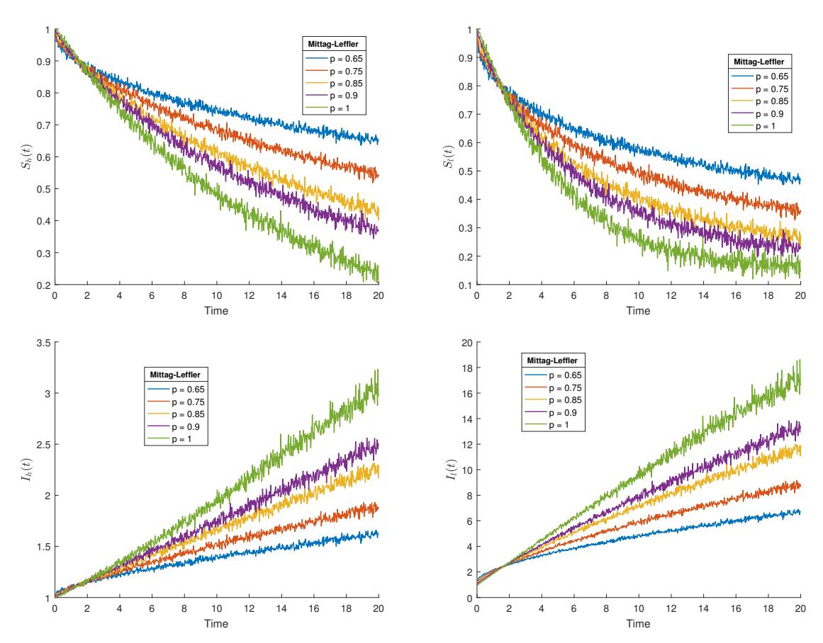
Figure 1: Numerical simulation results of model (6) based on AB operator order derivative for five arbitrary values of the order p and stochastic constants bi = 0.2, 0.25, 0.4, 0.5, 0.7, 0.75, 0.8, 0.85.
Figure 2(a) depicts recovered high status individuals Rh(t) and the number of individuals initially increased within the first 3 days. The ensuing days, as the fractional order derivative appreciates towards the integer order, the recovered individuals reduce for the rest of the 17 days. Figure 2(b), is the recovered low status individuals Rl and for the first three days the recovered individuals increased. For the rest of the 17 days, the number of recovered low status individuals reduced as the fractional order derivative gets closer to the integer order. Figure 2(c) depicts the number of susceptible vectors (Sv) and it reduces as the fractional order derivative appreciates towards the integer order. Thus, this is typically associated with epidemiological models. Figure 2(d) depicts the number of infected vectors (Iv) and as the fractional order derivative appreciates towards the integer order the infectious vector population increases in the community.
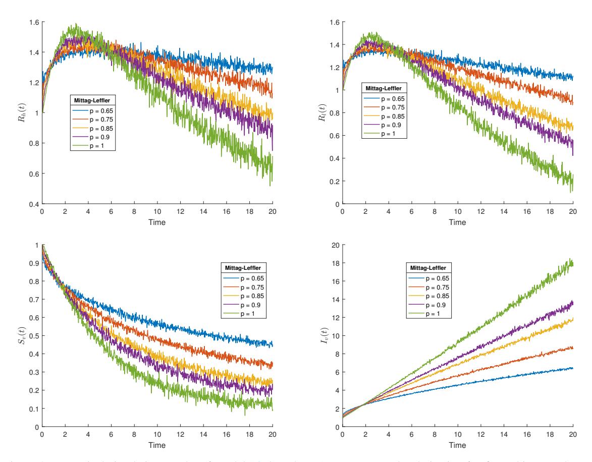
Figure 2: Numerical simulation results of model (6) based on AB operator order derivative for five arbitrary values of the order p and stochastic constants bi = 0.2, 0.25, 0.4, 0.5, 0.7, 0.75, 0.8, 0.85.
This study tries to compare the numerical simulation results of the adopted malaria model and this fractionalised model. The numerical simulation results of the model depicts the randomness which indicates the fluctuations in each compartments. This randomness is in line with Din et al., [17] in their dengue fever model. The integer order models as in [25] show a linear relationship with time domain. The randomness in reality shows how changes in the dynamics in epidemiology occurs. The high and low malaria status numerical simulation result presented in [25] indicate that the infection reduces with time however, in this work, both high and low status individuals increase with time. This supports the concept of memory effect that provides room for fractional derivative operator ML to thrive. In same manner, the susceptible vector compartment of the [25] and the current work is in opposite direction. In this work, as the susceptible vectors decrease, at the same time in their work the number of susceptible vectors increase. This again explains the two different concepts of integers and non-integers.
6. CONCLUSION
This studied examined the malaria dynamics with emphasis on status class in the society of a fractionalised system. The work was solely based on the new operator characterised by non-local and non-singular kernel. The positivity of the malaria model solution was proven. The existence and uniqueness of solutions had been studied in both fractional deterministic and stochastic domains. Both results established the existences and uniqueness of solutions of the status class malaria model. The numerical scheme based on Newton polynomial was used to present the numerical results to support the analytical results. It was observed that the susceptible classes decreased with respect to time. The dynamics of malaria status model indicated that the fractional order derivative had a serious effect on the dynamics of the various compartments. Thus, the variations of the fractional order derivatives provided the direction of whether or not as the fractional order increases or reduces directly or indirectly influenced the compartment. It is suggested that fractional derivative based on Mittag-Leffler function can be utilised in solving other complex models. Generalized Mittag-Leffler function is non-singular and non-local therefore predicts accurately from the origin which leads to accurate prediction.
ACKNOWLEDGEMENT
Parts of this article were funded by research grant.