Application of the Fractional Calculus in Pharmacokinetic Compartmental Modeling

1. INTRODUCTION

Pharmacokinetics have been defined as the flow and rate of distribution and removal of a drug or nanoparticle (NP) inside body. Pharmacokinetics may be represented as mathematical models to determine the process of administered drug movement throughout body. Pharmacokinetics models are the main piece of modeling based drug development and can be performed by non-compartmental or compartmental methods. Compartmental modeling helps to find the most efficient route of drug administration based on time of uptake and elimination [1], [2], [3]. These models provide a theoretical and mathematical framework to demonstrate the transmit of molecules biochemistry and transport phenomena in the body, and it has been done by dividing body into two main compartments based on pharmacokinetic and pharmacodynamic of different tissues. Therefore, compartmental modeling defines a comprehensive framework which makes an effective drug delivery toward targeted tissue and has been attracted by different researchers to find the most optimized therapy for different diseases such as cancer [4], [5], [6]. These models receives information regarding route of administration such as intravenous or intramuscular injection, and or oral and combine them by different assumptions related to single or multiple doses to demonstrate drug traveling states inside body, starting from the absorbing by tissue and distributing from one organ to the other organ, and then chemical alteration of the specific tissue, and finally declining drug concentration because of elimination of chemical or biochemical drug by all removal paths [1], [2], [3], [4], [5], [6].

Another approach to simulate distribution of drug in body that involves different organs and their interactions with other tissues called physiologically based pharmacokinetics models (PBPK) [1], [2]. This computer

based modeling method receives biological information such as physiological and chemical parameters for administered drug, blood flow rates to different tissues, volume of different organs, absorption and metabolism parameters, exposure and dose parameters and depends on different administration route, predicts the concentration of drug in different tissues using computational and numerical tools [1], [2], [3].

To understand the (ADME) process of drugs in different tissues mathematical and statistical models have been used by many different researchers [7], [8], [9], [10]. These models use differential equation framework which are well-defined based on frequency responses [6], [5], but should be appropriately scaled because of sensitivity of drugs to body mass of adults which is an index of body fat measurement in terms of weight or height of different persons [6]. However, to build a comprehensive computational model, we need to obtain different experimental data which demonstrates the (ADME) process in different body organs [6], [5], [11], [12], [13]. Basically, these models provide us more flexibility in analysis and then modification and update by converting given biological system including all parameters into a mathematical model which can be written as the form of deterministic or stochastic differential equations (ODE,PDE). For example, a PBPK model is a mathematical model and structural framework which explains the (ADME) process of drugs in different tissues such as kidney, liver, lung, muscle, plasma, and so on. One of the advantages of this type modeling is preserving the same physiological parameters as the original system during modeling process.

During the recent years, the area of fractional calculus has been attracted by many researchers in biology and medicine [14], [15], [16], [17], chemistry and biochemistry [18], [19], [20], physics and engineering [21], [22]. Due to wide applications of fractional modeling in science, and engineering, its importance and popularity is increasing day by day and it has allocated many attentions [14], [15], [16], [18], [19], [20], [17], [22], [21]. Fractional calculus is a new approach for modeling biological and physical phenomena with memory effects. Fractional calculus uses differential and integral operators including non-integer orders to study the non-linear behavior of physical and biological systems with some degrees of fractionality or fractality. While the integer order models provide a small class of non-integer order models, using fractional-order operators, we can study different classes of the same model through changing the fractional-order. Therefore, these models provide us more flexibility to analyze and control the behavior of a system.

There are many studies that proved the fractional-order differential equations (FODEs) and or models with integral operators provide more precise results in real world applications since there are some biological or physical systems which display memory in their long term behavior and the traditional ODEs of integer-order disregard this fact [18], [22]. However, analytical solutions of these equations cannot explicitly be obtained. Therefore, to find the dynamical behaviors of solutions, we require to use approximation and numerical schemes. The finite difference method, adomian decomposition method, extrapolation method, multistep method, iterative methods, and predictor corrector techniques can be used to acquire the numerical simulations of the linear and non-linear FODEs.

Here, we want to explore the behaviors of the solutions of three pharmacokinetic compartmental models and their corresponding fractional-order forms. We organize this study as follows: to drive the fractional-order compartmental models, we apply the nonstandard finite difference (NSFD) method since they provide better results compare to traditional standard finite difference (SFD) methods and then we discretize these pharmacokinetic compartmental models using the Grunwald-Letinkov discretization method. We use the numerical methods to demonstrate (ADME) process for any drug in different compartments in both original and fractional-order models. By considering the fractional-order framework in pharmacokinetic modeling, we can explain all the possible geometric mechanisms underlying drug distribution in different tissues.

2. MATHEMATICAL BACKGROUND

Fractional calculus as a field of mathematics can be considered as an old and novel topic [23], [24], [25], [26]. To introduce some of the widely used fractional derivatives and integrals of a function f(x) of arbitrary order \(\alpha\), we start with definition of fractional integral in the sense of Riemann and Liouville. According to Riemann-Liouville, fractional integral of order \(\alpha\) (\(\alpha > 0\)) may be defined as a natural consequence of Cauchy formula:

\[J^{n}f(t) := f_{n}(t) = \frac{1}{(n-1)!} \int_{0}^{t} (t-s)^{n-1} f(s) ds, \quad t > 0, \quad n \in \mathbb{N},\] (1)

where \(f_n(t)\) vanishes at t=0 with its derivatives of order \(1, 2, \ldots, n-1\). Using the Gamma function,

Definition 2.1. The gamma function is defined as follows:

\[\Gamma(x) = \int_0^\infty y^{x-1} e^{-y} dy,\tag{2}\] where for convergence of the integral, x > 0.

We can extend (1) from positive integer values to any positive real values and for \(\alpha > 0\) write it as:

Definition 2.2 (Riemann Liouville integral, Riemann (1953) and Liouville (1832)). The fractional integral of order \(\alpha \in \mathbb{R}^+\) of the function f(t), for t > 0 where \(f : \mathbb{R}^+ \to \mathbb{R}\) has been defined by

\[I_a^{\alpha} f(t) = \frac{1}{\Gamma(\alpha)} \int_a^t (t-s)^{\alpha-1} f(s) \, ds, \qquad t > 0.\] (3)

Definition 2.3 (Riemann-Liouville fractional derivative). [27] The fractional derivative of order \(\alpha \in (n-1, n)\) of f(t) is defined by taking fractional integral of order \((n-\alpha)\), and then take nth derivative as follows:

\[D_*^{\alpha} f(t) = D_*^n I_a^{n-\alpha} f(t), \tag{4}\] where

\[D_*^n = \frac{d^n}{dt^n}, \qquad n = 1, 2, \dots\] (5)

Then, we define the Grunwald-Letinkov definition of fractional derivative:

Definition 2.4 (Grunwald-Letinkov fractional derivative, Grunwald and Letinkov 1872). [28] The Grunwald-Letinkov definition of fractional derivative of a function generalizes the notion of backward difference quotient of integer order. In this case \(\alpha=1\) if the limit exists the Grunwald-Letinkov fractional derivative is the left derivative of the function. The Grunwald-Letinkov fractional derivative of order \(\alpha\) of the function f(x) is define as

\[D_x^{\alpha} f(x) = \lim_{N \to \infty} \frac{(x-a)^{-\alpha}}{\Gamma(-\alpha)} \sum_{j=0}^{N-1} \frac{\Gamma(j-\alpha)}{\Gamma(j+1)} f(x-j\left[\frac{x-a}{N}\right]). \tag{6}\]

If \(\alpha = -1\), we have a Riemann sum. If \(\alpha = 1\), then we have

\[\lim_{N \to \infty} \frac{f(x) - f(x - \left[\frac{x - a}{N}\right])}{\left[\frac{x - a}{N}\right]},\tag{7}\] which is left derivative of the function f at x.

In 2015, Caputo and Fabrizio proposed a new derivative with fractional-order [29] with two different forms, however, the first representation was proposed by Joseph Liouville in 1832 [27], [30]. Caputo's representation which is a modification of the Riemann Liouville definition and can be used for initial value problems, has the following definition:

Definition 2.5 (Caputo-fractional derivative, Caputo (1967)). [29] The fractional derivative of order \(\alpha \in (n-1,n)\) of f(t) is defined by taking \(n^{th}\) derivative. Next, we use the fractional integral operator of order \((n-\alpha)\),

\[D^{\alpha} f(t) = I_a^{n-\alpha} D_*^n f(t), \qquad n = 1, 2, \dots\] (8)

Therefore, Caputo derivative of order \(\alpha\) has the form:

\[D^{\alpha}f(t) = \frac{1}{\Gamma(n-\alpha)} \int_0^t \frac{f^n(s)}{(t-s)^{\alpha-n+1}} ds, \tag{9}\] where \(n-1 < \alpha < n\), n is an integer, and \(f^n\) is nth derivative of f(s).

In the definition of fractional derivative with respect to time of any map f(t) at t = tn, we perform an integral operator and then we compute the fractional derivative with respect to time for which we need to know the history of the system equations (knowing the values of f(t) in the interval t ∈ [0, tn]. A common approach to solve the problems with the Caputo fractional-derivative operator is using the Laplace transform. The Laplace transform formula for the Caputo fractional-derivative operator has the following form

\[\mathcal{L}\{D^{\alpha}f(t)\} = z^{\alpha}F(z) - \sum_{k=0}^{n-1} z^{\alpha-k-1}f^{(k)}(0), \tag{10}\] where f (k) (0) is the initial conditions of f(t). If we neglect the initial conditions, we get

\[\mathcal{L}\{D^{\alpha}f(t)\} = z^{\alpha}F(z). \tag{11}\]

From (11) and using the definition of Laplace transform of Riemann Liouville fractional integral:

\[\mathcal{L}\{I^{\alpha}f(t)\} = z^{-\alpha}F(z),\tag{12}\]

we get the definition of general differintegral fractional operator as:

\[\mathcal{L}\{D^{\pm\alpha}f(t)\} = z^{\pm\alpha}F(z). \tag{13}\]

It has been proved that for the most analytic functions, Grunwald-Letnikov fractional derivative is identical to Caputo fractional derivative. The difference between the Grunwald-Letnikov definition and Caputo definition appears when dealing with constant function. For example, for a constant function, the Caputo fractional derivative is zero while its RiemannaLiouville fractional derivative is not. In the application, Caputo fractional ˆ derivative has been used for initial value fractional ordinary differential equations. For the case α is an integer, the fractional derivative would be identical to the integer derivative and we can conclude that fractional calculus is a kind of interpolation of the integer calculus. One important fact about fractional operators such as fractional integral and fractional derivative is that there has not been developed any acceptable physical and or geometrical interpretation for these operators during 300 years [30].

3. PHARMACOKINETIC TWO COMPARTMENTAL MODEL

To demonstrate the uneven transition of drug in body, we use a bi-compartmental model which follows a biexponential distribution to describe disposition of drugs. We start with the simplest case when we assume that drugs distribute from second compartment or capillary bed into the third compartment or tissue compartment but they would be eliminated from the second compartment (see the schematic diagram in Figure (1)).

Figure 1: Schematic diagram of a simple bi-compartmental model for drug distribution, where k²³ and k³² represent the rate of drug distribution between compartment two or capillary bed and three or tissue, k²⁴ is the rate of elimination from vascular capillary bed to the venous.

Here, transfer rate constants k²³ and k32, milligram per minute (mg/min), illustrate the reversible transfer of drugs between compartment two and compartment three. In general, this is a simplification of (ADME) procedure in the whole body. In this case, we consider that drug concentration initially decreases very fast and they distribute rapidly into the tissue compartment. Here, tissue compartment may be contained several organs in body. After this phase, there would be an equilibrium phase for drug concentration in which concentration of them decreases so slowly, and therefore we only have elimination of these particles.

In this bicompartmental model, we consider a transfer rate of first order between second and third compartments and also we assume that elimination of drug from the second compartment or capillary bed follows a rate of first order, and lastly, we ignore any other metabolism in capillary bed. To demonstrate distribution of drugs in Figure (1), we write the following kinematic equations,

\[\begin{cases} \frac{1}{V_2} \frac{dA_2}{dt} = \frac{-k_{23} A_2}{V_2} + \frac{k_{32} A_3}{V_3} - \frac{k_{el} A_2}{V_2}, \\ \frac{1}{V_3} \frac{dA_3}{dt} = \frac{-k_{32} A_3}{V_3} + \frac{k_{23} A_2}{V_2}, \end{cases} (14)\]

where, A² and A³ are the drug concentrations in compartment two or capillary bed and compartment three or tissue respectively molar units (e.g. µmol) per unit volume, and V² and V³ represent the volume of compartment two and three respectively.

We assume that at t = 0, A³ = 0, i.e. the drug concentrations in tissue is zero. Therefore, we have the following boundary conditions for the equations (14) at t = 0,

\[A_2 = \frac{\mathsf{Dose}}{V_2}, \quad A_3 = 0.\]

Therefore, after solving Model (14), we find the concentration of drug in capillary bed, A2, and tissue, A3, as the form,

\[\begin{cases} A_{2} = \frac{\operatorname{Dose}\left[\left(k_{32} - r_{1}\right)e^{-r_{1}t} - \left(k_{32} - r_{2}\right)e^{-r_{2}t}\right]}{V_{2}(r_{2} - r_{1})}, \\ A_{3} = \frac{\operatorname{Dose}\left(k_{23}\left[e^{-r_{2}t} - e^{-r_{1}t}\right]\right)}{V_{2}(r_{1} - r_{2})}, \end{cases} (15)\] where,

\[\text{[rumus tidak dapat ditampilkan dengan baik — lihat PDF asli]}\]

The first order constants r¹ and r² determine if drug distribution and removal take place slow or fast and from (16) we can see that they depend on constant rates k23, k32, and kel.

The following equality describes the relationships between r¹ and r² and three rates k23, k³² and kel;

\[\frac{r_1 + r_2}{r_1 \, r_2} = \frac{k_{23} + k_{32} + k_{el}}{k_{32} \, k_{el}}.\]

Using mathematical modeling not only helps us to find the concentration of drug in different compartments, but also helps to approximate distribution rates between different compartments. The concentration of drug in capillary bed of Model (14) can be simply obtained by adding the amount of drug that is sent to the tissue and the amount of drug that is eliminated from capillary:

\[A_2 = A(Distribution) + A(Elimination).\]

Thus,

\[A_2 = \eta_1 e^{-r_1 t} + \eta_2 e^{-r_2 t},\] where, A² consists of two phases, first the exponential term η¹ e −r¹ t related to distribution phase and η² e −r² t related to elimination phase of drug from compartment two. In Model (14), because distribution is faster than removal, therefore, we assume that the exponential term η¹ e −r¹ t is zero and we rewrite A² as

\[A_2 = \eta_2 \, e^{-r_2 \, t}.\]

If we convert it to log form, we have

\[\log A_2 = \log \eta_2 - \frac{r_2 t}{2.303}.\]

Moreover, for this simple case, we can easily evaluate pharmacokinetic parameters, k23, k³² and kel.

3.1. Grunwald-Letinkov approximation for bicompartmental Model (14)

The fractional differential operator has the following form [31], [32],

\[D^{\gamma}A(t) = f(t, A(t)), \quad A(t_0) = A_0,\] where γ > 0 represents the order of derivative and D^γ denotes the fractional derivative which is given by:

\[D^{\gamma}A(t) = J^{k-\gamma}D^kA(t),\] where γ ∈ (k − 1, k], for k = 1, 2, . . . and integral operator J k called the Riemann-Liouville operator of kth-order which is obtained by the following formula

\[J^{k}A(t) = \frac{1}{\Gamma(k)} \int_{0}^{t} (t - \tau)^{(k-1)} A(\tau) d\tau, \quad t > 0,\] where Γ(.) denotes the gamma function. To apply the Micken's (NSFD), we need to find the fractional-order derivative using the Grunwald-Letinkov (G-L) approximation for Model (14) as the form [33], [34], [35]

\[D^{\gamma} A(t) = \lim_{s \to 0} s^{-\gamma} \sum_{i=0}^{T} (-1)^{i} {\gamma \choose i} A(t - i s), \tag{16}\] where T = [t]/s and [.] used to show the integer value and s represents the step size. Thus, Equation (16) would be discretized as

\[\sum_{i=0}^{T} C_i^{\gamma} A(t_{k-i}) = f(t_k, A(t_k)), \tag{17}\]

where t^k = k s and C γ i are the coefficients for (G-L) approximation written as

\[C_i^{\gamma} = \left[\frac{i-1-\gamma}{i}\right]C_{i-1}^{\gamma}, \quad C_0^{\gamma} = s^{-\gamma} \quad i = 1, 2, \dots\]

Next we introduce the non standard finite difference procedure.

3.2. Non-standard discretization of bicompartmental Model (14)

To discretize a system of differential equations (DEs) including a system of ordinary differential equations (ODEs) and or a system of partial differential equations (PDEs), one may apply the Mickens NSFD discretization method which is more flexible in construction rather than standard finite difference method and therefore has better performance. This method checks the positivity of solutions and is concerned about boundedness and monotonicity of them. Another advantage of using NSFD schemes is their ability to preserve the structure and properties of the system of differential equations and therefore, we apply NSFD schemes on the general compartmental model of the form:

\[\frac{dA}{dt} = f(A). (18)\]

However, to apply the non-standard scheme we need to check that if non-local approximation is used and or we need to have a non traditional discretization of derivatives and also we may need to use a non-negative function \(\Phi(h) = s + O(s^2)\). To apply NSFD scheme, we consider a grid \(t_k = t_0 + k s\), such that s > 0, and we approximately write the discretized function A as \(A_k \approx A(t_k)\). Next, we discretize (18):

\[\frac{dA}{dt} = \frac{A_{k+1} - A_k}{\Phi(s)} + O(\Phi(s)), \quad \text{when} \quad s \to 0 \quad \Longrightarrow \quad \frac{dA}{dt} \approx \frac{A_{k+1} - A_k}{\Phi(s)}, \tag{19}\] where real valued \(\Phi(s)\) as a function of the step size s needs to satisfy the following properties:

\[\Phi(s) = s + O(s^2), \quad \Phi(s) \in (0, 1), \quad \forall s \in (0, \infty).\] (20)

Here, the equality (19) is equivalent with the integer order derivative because:

\[\begin{split} \frac{dA}{dt} &= \lim_{s \to 0} \left[ \frac{A(t+s) - A(t)}{\Phi(s)} + O(\Phi(s)) \right], \\ &= \lim_{s \to 0} \left[ \frac{A(t+s) - A(t)}{s} \right] \lim_{s \to 0} \left[ \frac{s}{\Phi(s)} \right] + \lim_{s \to 0} O(\Phi(s)) = \dot{A}(t). \end{split}\]

As \(s \to 0\) the discrete form in (19) converges to its associated continuous derivative. NSFD methods are convergent without any restriction related to step size s but this is not always true for SFD methods which depend on the step size s. Moreover, when we discretize a system using NSFD method, if the original system is persistent, and solutions are stable and convergent, these properties remain the same after discretization, but not for the case we use SFD to discretize the system of differential equations.

3.3. Fractional Bicompartmental Model

Finally to apply the Mickens NSFD method, we substitute the step size s by \(\Phi(s)\). Next, we use the G-L technique to discretize the equations (16). We consider \(A_2(t_k) = A_2^k\), \(A_3(t_k) = A_3^k\), we have:

\[\begin{cases} \frac{1}{V_2} \sum_{i=0}^{k+1} C_i^{\gamma} A_2^{k+1-i} = \frac{-k_{23} A_2}{V_2} + \frac{k_{32} A_3}{V_3} - \frac{k_{el} A_2}{V_2}, \\ \frac{1}{V_3} \sum_{i=0}^{k+1} C_i^{\gamma} A_3^{k+1-i} = \frac{-k_{32} A_3}{V_3} + \frac{k_{23} A_2}{V_2}. \end{cases} (21)\]

After simplification, the fractional-order system which is linear and time-invariant has the following form:

\[\begin{cases} A_2^{k+1} = \left[ \frac{k_{32} A_3}{V_3} - \frac{\sum_{i=1}^{k+1} C_i^{\gamma} A_2^{k+1-i} + k_{23} A_2 + k_{el} A_2}{V_2} \right] \frac{V_2}{C_0^{\gamma}}, \\ A_3^{k+1} = \left[ \frac{k_{23} A_2}{V_2} - \frac{\sum_{i=1}^{k+1} C_i^{\gamma} A_3^{k+1-i} + k_{32} A_3}{V_3} \right] \frac{V_3}{C_0^{\gamma}}. \end{cases} (22)\]

We have demonstrated the solutions of the fractional-order system (22) for different orders in Figures (2) and (3).

4. BICOMPARTMENTAL MODEL WITH DRUG INFUSION

For this case, we have the following two compartmental model (see Figure (4)),

\[\begin{cases} \frac{1}{V_2} \frac{dA_2}{dt} = \frac{k_{12} A_1}{V_1} + \frac{-k_{23} A_2}{V_2} + \frac{k_{32} A_3}{V_3} - \frac{k_{el} A_2}{V_2}, \\ \frac{1}{V_3} \frac{dA_3}{dt} = \frac{-k_{32} A_3}{V_3} + \frac{k_{23} A_2}{V_2}. \end{cases}\] (23)

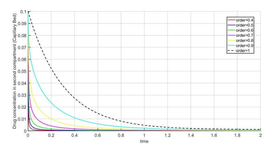
Figure 2: Evolution of drug concentration in capillary bed in fractional-order bi-compartmental model (22) for orders γ = 0.4 - γ = 1 and the initial conditions k²³ = .8, k³² = 0.03, kel = 1.5, the drug concentration for all compartments to be 1. In this model, the constant rates k23, k32, and kel determine the fast drug distribution and slow drug elimination.

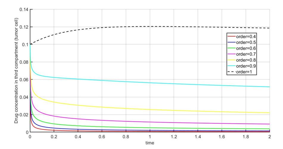
Figure 3: Evolution of drug concentration in tissue in fractional-order bi-compartmental model (22) for orders γ = 0.4 γ = 1 and the initial conditions k¹² = 1, k²³ = .8, k³² = 0.03, kel = 1.5, the drug concentration for all compartments to be 1.

A¹ is the concentration of drug in compartment one, V¹ is the volume of compartment one, and k¹² is drug infusion rate. For Model (23), we can derive A² as the form,

\[A_2 = \frac{k_{12}}{V_2 k_{el}} \left[ 1 + \frac{k_{el} - r_2}{r_2 - r_1} e^{-r_1 t} - \frac{k_{el} - r_1}{r_1 - r_2} e^{-r_2 t} \right]. \tag{24}\]

At steady state, when t → ∞, e −r¹ t and e −r² t converge to zero and we have,

\[A_2 = \frac{k_{12}}{V_2 \, k_{el}} = \frac{\text{infusion rate}}{\text{clearance}}.\]

Figure 4: Schematic diagram of a simple bi-compartmental model for drug distribution, where k¹² describe the transition rate from artery to capillary, k²³ and k³² represent the rate of drug distribution between compartment two or capillary bed and three or tissue, k²⁴ is the rate of elimination from vascular capillary bed to the venous.

We define the Grunwald-Letinkov approximation as before to apply the non standard finite difference Micken's procedure and finding the following fractional-order system for (23):

\[\begin{cases} A_2^{k+1} = \left[ \frac{k_{12} A_1}{V_1} + \frac{k_{32} A_3}{V_3} - \frac{\sum_{i=1}^{k+1} C_i^{\gamma} A_2^{k+1-i} + k_{23} A_2 + k_{el} A_2}{V_2} \right] \frac{V_2}{C_0^{\gamma}}, \\ A_3^{k+1} = \left[ \frac{k_{23} A_2}{V_2} - \frac{\sum_{i=1}^{k+1} C_i^{\gamma} A_3^{k+1-i} + k_{32} A_3}{V_3} \right] \frac{V_3}{C_0^{\gamma}}. \end{cases} (25)\]

The numerical solutions of the fractional-order system (25) of different orders have been demonstrated in Figures (5) and (6).

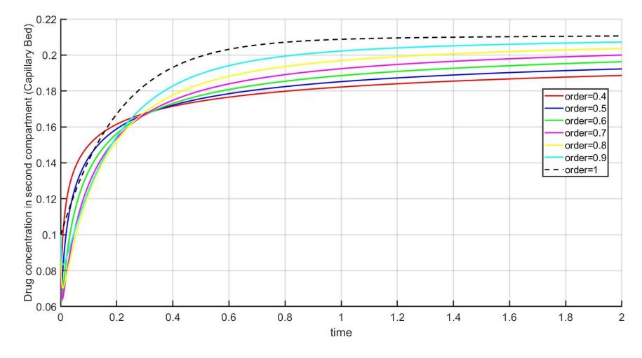
Figure 5: Evolution of drug concentration in capillary bed in fractional-order bi-compartmental model (25) for orders γ = 0.4 - γ = 1 and the initial conditions k¹² = 1, k²³ = 0.8, k³² = 0.03, kel = 1.5, the drug concentration for all compartments to be 1.

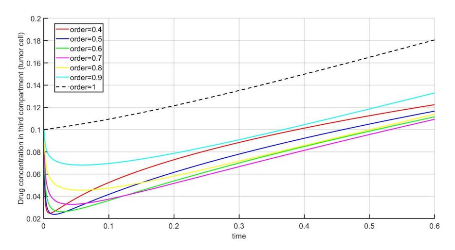
Figure 6: Evolution of drug concentration in tissue in fractional-order bi-compartmental model (25) for orders γ = 0.4 γ = 1 and the initial conditions k¹² = 1, k²³ = 0.8, k³² = 0.03, kel = 1.5, the drug concentration for all compartments to be 1.

5. APPLICATIONS OF FRACTIONAL CALCULUS TO MODEL DRUG DIFFUSION IN A THREE COMPARTMENTAL PHARMACOKINETIC MODEL

Inside our body, the blood vessels are covered with specific cell types called Endothelial cells (ECs). Therefore, we have added a new compartment to the previous two compartmental model to have a more realistic model. These cells based on their size and location play different roles in our body. For example, some of them carry small size molecules and or specific hormones such as insulin, the others are effective in regulation of blood pressure. However, all of these cells have a common role that is building a wall between blood cells and other tissue cells [36]. For simplicity, we ignore their interactions with surrounding cells.

We consider a new compartmental model with three compartments to represent (ADME) of drugs as it is demonstrated in Figure (7). In this case, we assume that we have three phases; absorption and distribution,

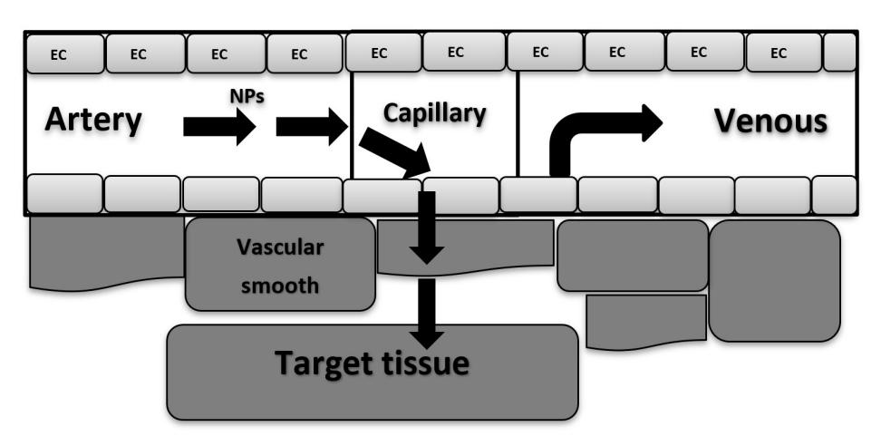
Figure 7: EC or endothelial cells as a barrier between body vessels and different tissues facilitate the transportation of drug from capillary to tissue.

Figure 8: Schematic diagram of the three compartmental pharmacokinetic model for drug disposition, where \(k_{23}\), \(k_{32}\)and \(k_{34}\) represent the constant rates of transfer between the indexed compartments, \(k_{25}\) stands for the mass transfer rate from vascular in the second compartment to the venous.

and leakage or elimination. Drugs enter from artery which is the first compartment to the capillary or second compartment with absorption rate \(k_{12}\). Next, we have distribution to the third compartment or Endothelial cells with a rate \(k_{23}\). Then, we have transition of drugs into tissue with transfer rate \(k_{34}\):

\[\begin{cases} \frac{1}{V_2} \frac{dA_2}{dt} = \frac{k_{12} A_1}{V_1} + \frac{-k_{23} A_2}{V_2} + \frac{k_{32} A_3}{V_3} - \frac{k_{el} A_2}{V_2}, \\ \frac{1}{V_3} \frac{dA_3}{dt} = \frac{-k_{32} A_3}{V_3} + \frac{k_{23} A_2}{V_2} - \frac{k_{34} A_3}{V_3}, \\ \frac{1}{V_4} \frac{dA_4}{dt} = \frac{k_{34} A_3}{V_3}, \end{cases} (26)\]

where, \(A_4\) is the concentration of drug in deep tissue or compartment four, \(V_4\) is the volume of compartment four, and \(k_{34}\) is the reversible transfer of drug between compartment three and four, see Figure (8). After solving Model (26) for \(A_3\) and \(A_4\) we have:

\[A_2 = M_2, \tag{27}\]

\[A_3 = \frac{M_2 k_{23}}{k_{32} + k_{34}} \left[ 1 - e^{-(k_{32} + k_{34})t} \right] + A_3(0) e^{-(k_{32} + k_{34})(t - \Gamma)}, \tag{28}\]

\[A_{3} = \frac{M_{2} k_{23}}{k_{32} + k_{34}} \left[ 1 - e^{-(k_{32} + k_{34})t} \right] + A_{3}(0) e^{-(k_{32} + k_{34})(t-\Gamma)},\] \[A_{4} = \frac{M_{2} k_{23} k_{34}}{k_{32} + k_{34}} \left[ t - \frac{1 - e^{-(k_{32} + k_{34})t}}{k_{32} + k_{34}} \right] + \frac{k_{34} A_{3}(0)}{k_{32} + k_{34}} \left[ 1 - e^{-(k_{32} + k_{34})t(t-\Gamma)} \right] + A_{4}(0).\] (29)

As before, we apply the NSFD Micken's method and we find the following fractional-order system for (26):

\[\begin{cases} A_2^{k+1} = \left[ \frac{k_{12} A_1}{V_1} + \frac{k_{32} A_3}{V_3} - \frac{\sum_{i=1}^{k+1} C_i^{\gamma} A_2^{k+1-i} + k_{23} A_2 + k_{el} A_2}{V_2} \right] \frac{V_2}{C_0^{\gamma}}, \\ A_3^{k+1} = \left[ \frac{k_{23} A_2}{V_2} - \frac{\sum_{i=1}^{k+1} C_i^{\gamma} A_3^{k+1-i} + k_{32} A_3 + k_{34} A_3}{V_3} \right] \frac{V_3}{C_0^{\gamma}}, \\ A_4^{k+1} = \left[ \frac{k_{34} A_3}{V_3} - \frac{\sum_{i=1}^{k+1} C_i^{\gamma} A_4^{k+1-i}}{V_4} \right] \frac{V_4}{C_0^{\gamma}}. \end{cases} (30)\]

We have demonstrated the numerical solutions of the fractional-order system (30) of different orders in Figures (9) - (11).

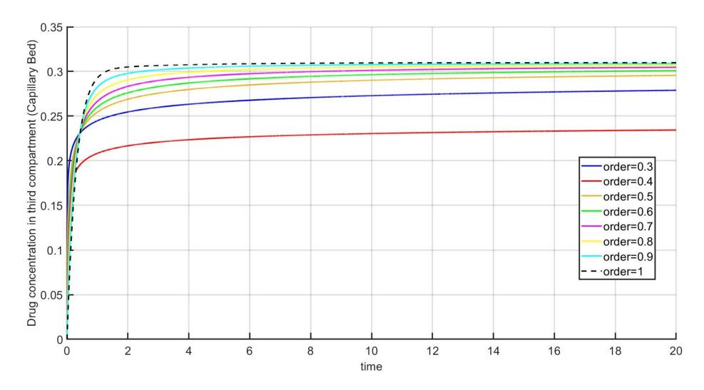
Figure 9: Evolution of drug concentration in capillary bed in fractional-order tri-compartmental model (30) for orders γ = 0.3 - γ = 1 and the initial conditions k¹² = 1, k²³ = 0.8, k³² = 0.03, kel = 1.5, k³⁴ = 0.3, the drug concentration for all compartments to be 1.

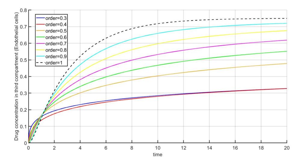
Figure 10: Evolution of drug concentration in endothelial cells in fractional-order tri-compartmental model (30) for orders γ = 0.3 - γ = 1 and the initial conditions k¹² = 1, k²³ = 0.8, k³² = 0.03, kel = 1.5, k³⁴ = 0.3, the drug concentration for all compartments to be 1.

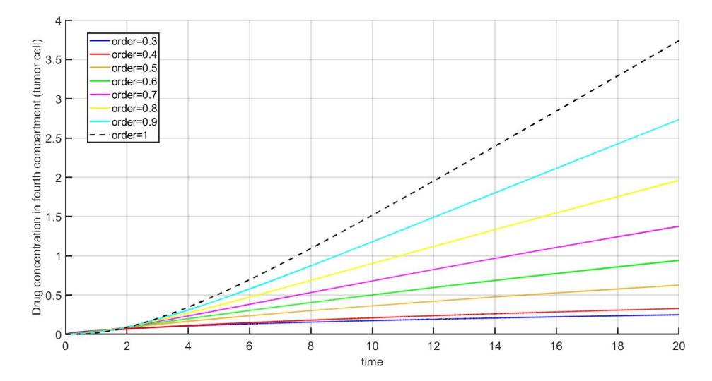
Figure 11: Evolution of drug concentration in tissue in fractional-order tri-compartmental model (30) for orders γ = 0.3 - γ = 1, and the initial conditions k¹² = 1, k²³ = 0.8, k³² = 0.03, kel = 1.5, k³⁴ = 0.3, the drug concentration for all compartments to be 1.

6. RESULT AND DISCUSSION

Pharmacokinetic compartmental models play an important role to study the chemical or biochemical reactions of drugs and their distribution entire body and to measure the rates of distribution in different tissues. Pharmacokinetic compartmental models have been used widely to demonstrate how chemical compounds such as drugs interact with biological processes in different tissues. Pharmacokinetic models are often represented as the form of differential equations. There are many studies related to cancer therapy that use the compartmental models to approximate the drug concentration in tumor cells and other tissues. These models are concerned about different pathways to administer drug and compare them to find the concentration of chemicals in different tissue that helps to explore the best route of drug administration for different diseases and finally better treatment. Fractional calculus is a new approach for modeling physical and biological phenomena with memory or aftereffects. Fractional calculus uses differential operators and integral operators of orders that are not integer to study the complexity and behavior of non-linear physical and biological systems which display some degrees of fractional and fractal behavior. Using fractional derivatives and integrals we are able to explain the memory and patrimonial effect in different events and successive processes in real world phenomena. Since the analytical and explicit solutions of fractional ordinary differential equations (FODEs) (linear and non-linear forms) cannot be easily obtained, someone needs to use computational methods and computer simulations to approximate the solutions of these systems. fractional-order modeling in biology and specifically physiology helps to explore the complexity of different processes inside human body and to characterize and measure different organs complication using fractal geometry and fractional calculus tools. Moreover, since tumor cells interactions are systems with memory, therefore FODEs are better candidates to model cancer phenomena rather than ordinary and delay differential equations.

In the current research, we have explored the process of drug distribution inside the body using three different pharmacokinetic compartmental models. These models include physiological parameters which describe the process of ADME of drug in different body organs. At first, we have considered integer order compartmental models to display the process of drug distribution in different tissues tissue. We tried to write the mathematical models using the schematic diagrams that makes it easier to study these biological processes. Next, we have used the Grunwald-Letinkov discretization method to discretize these pharmacokinetic compartmental models. Finally, to obtain the fractional-order compartmental model for each case, we have applied the nonstandard finite difference method (NSFD) Micken's technique. To compare the solutions of fractional-order systems of different orders to the corresponding traditional integer order models, we have carried out some numerical methods (by preserving the same biological parameters) since the solutions of fractional-order models may not be explicitly obtained. The graphical presentations of numerical results showed that NSFDM is easy and convenient to implement, and effective enough for solving efficiently the proposed models. Therefore, these numerical results would be a good starting point to find out the best mathematical model to demonstrate the absorption, distribution, and excretion of drug in different body organs. By considering the fractional-order modeling approach, we could improve the capabilities of the integer order modeling into the generalized domain of fractional calculus and we could derive all the possible geometric mechanisms underlying the (ADME) of drug inside body. Likewise, we have used the order of fractional derivative as a new control parameter to extract the variety of governing classes on the non-local behaviors of these models (since for each order we have a new model), while, the integer order framework only could study the local behaviors in the integer order domain. Using the order of fractional derivative, we can see different classes of the model and select the model that can be a perfect fit for our data. It also gives us more control to write down a model that is closer to our experimental results or to choose the appropriate order that demonstrates the expected dynamical behaviors.

The fractional-order approach discussed in this study required to be extended to be an appropriate framework in the pharmacokinetic modeling area. In principle, it is worthwhile to mention the limitations of this work. Because the experimental data was not available for this study, future work is crucial to evaluate how reliable is the provided fractional-order models. Using the experimental data would significantly improve the reliability of this framework for drug diffusion modeling. It is straightforward to apply fractional calculus on the pharmacokinetic compartmental model representations proposed here, however we may require to find a concrete and rigorous analysis to discover the relevance of the physiological interpretation of the fractional differentiation order γ as a newly added parameter. Although it is evident from numerical simulations that different classes of these compartmental models and their dynamics have mainly been presented and captured by different fractional-order γ value, it would be of great significance to find the ranges of γ value using experimental data for clinical applications.

ACKNOWLEDGMENT

The author would like to acknowledge the reviewers who helped to improve the current study.