

1. INTRODUCTION
In November 2019, the emergence of a new disease caused by the Coronavirus in Wuhan, China, shocked the world. Now, it is known as Coronavirus disease (Covid-19). The disease has similar initial symptoms to influenza, namely fever, cough, fatigue, sore throat, and difficulty breathing that can cause death [34]. Covid-19 can be transmitted from one individual to another easily through the droplets of infected individuals which contain Coronavirus. In a short time, there was a major outbreak in China and many countries all over the world. Therefore, The World Health Organization (WHO) announced Covid-19 as a global pandemic on March 2020 [33].
In order to decrease Covid-19 transmission, many strategies have been implemented such as quarantine of infected individuals, local lockdown, and minimizing the movement of people from one country to others. In addition to medical treatments and biological research about the virus itself, it is important to understand the dynamics of the disease transmission. Therefore, mathematical analysis is needed to study the factors which drive disease transmission and the effects of several control strategies before they are launched.
Many mathematical models have studied the transmission of Covid-19, starting from the SI and SIR models [8], [2]. The authors in [8] apply the SIR model to provide predictions for the spread of Covid-19 for the period of February until September 2020 by collecting data from several countries, namely Australia, USA, Italy, China, South Korea, and India, from February to June 2020. Meanwhile, the authors in [2] propose a model to predict Covid-19 using SIR and machine learning for smart health care and the welfare of Kingdom of Saudi Arabia (KSA) residents. Following the discovery that individuals exposed to the Coronavirus have an incubation period which lasts for a few days, a SEIR mathematical model was developed. In [5], the
*Corresponding author
Received August 3rd, 2021, Revised November 2nd, 2021, Accepted for publication February 17th, 2022. Copyright ©2022 Published by Indonesian Biomathematical Society, e-ISSN: 2549-2896, DOI:10.5614/cbms.2022.5.1.1
authors included vaccination parameters for susceptible individuals, with the assumption that Covid-19 will not infect any individual who has been vaccinated. In other words, the vaccine is able to prevent the infection completely. The authors in [15] propose the SEIR model and the AI model to predict the peak and size of the Covid-19 epidemic in the non-Wuhan region of mainland China. The results of this study indicate that if the lockdown is lifted, the outbreak in non-Wuhan areas in mainland China will double in size. Adjustments of those models were made to present the actual situation better. Furthermore, some studies divide infected individuals into symptomatic and asymptomatic compartments [23], [27]. Calculation of the basic reproduction number R0 is the main objective in those studies.
Recently, one of the strategies to decrease the transmission of Covid-19 is the vaccination program, including in Indonesia. Some works have studied the effects of vaccination on the spread of Covid-19. Ghostine et al. [17] considered the vaccinated population and quarantine policy in an improved Covid-19 model. In [17], the authors assumed that all infected individuals follow strict quarantine guidelines. In reality, since the number of infected people has increased rapidly lately, medical facilities cannot quarantine them in hospitals. In [22], Machado et al. also discussed a model with vaccination and without quarantine policy, but they considered the confirmed and unconfirmed infected populations. Savasan et al. [28] proposed a Covid-19 transmission model in Mediterranean Island by considering vaccination as well. In this work, they divided the infected population into three sub-populations, namely mild infected individuals that are in quarantine hotels, moderate infected individuals that are in hospitals, and severe infected individuals that are in intensive care units. In January 2021, the Indonesian government has launched a vaccination program for citizens. Fuady et al. [16] considered a model with a targeted vaccine allocation program in Indonesia without a quarantine strategy. However, those models have not been able to accommodate the fact that the efficacy of current vaccines is limited for a certain period of time in the body [10]. In [24], Omae et al. constructed a Covid-19 model to study the effects of vaccination by taking into account individuals with the first and second doses. They also considered the scenario that vaccinated people may move to the susceptible population again.
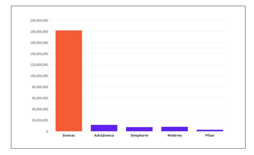
Figure 1: The number of doses of Covid-19 vaccines in Indonesia until September 2, 2021
Currently, there are several types of vaccines for Covid-19. Since the implementation of the national vaccination program to deal with Covid-19, since January 2021, Indonesia has used three types of vaccines until June 2021. Namely the CoronaVac (Sinovac), AstraZeneca, and Sinopharm [9]. Lately, the government of Indonesia has used other types of vaccines, such as Pfizer and Moderna. Until September 2021, Indonesia has used about 217 million doses of vaccines in total. From the 217 million doses, the Sinovac is the most commonly used vaccine in Indonesia, with about 181.9 million doses, followed by AstraZeneca with about 11.5 million doses. The complete data about the number of doses of Covid-19 vaccines in Indonesia until September 2021 is shown in Figure 1.
According to [19], each vaccine has a different efficacy, as seen in Table I. Since the efficacy of those vaccines varies even after getting vaccinated, people could be infected by the Coronavirus [35]. WHO also suggests keeping taking precautions to protect ourselves since some people may still get ill from Covid-19 after vaccination [35]. As such, there is an important question related to the eradication of Covid-19, i.e., whether it is enough to be vaccinated. The present study aims to analyze the effects of vaccination in controlling Covid-19 in Indonesia. For this reason, a vaccinated compartment will be added to the SEIR model, which will be one of the unique features of this study. Since vaccinated individuals may get ill from Covid-19, we assume that vaccinated individuals may become exposed (infected but not yet infectious) after contact with an infected individual. We also consider that the current vaccines only have efficacy for certain period of time. It is also assumed that vaccinated people have stronger immunity than susceptible unvaccinated people. In this study, the vaccine's efficacy affecting the immunity is represented implicitly by the infection rate. Thus, the infection rate for vaccinated people by the infected is lower than the infection rate for susceptible unvaccindated people. Additionally, we divide infected people into two sub-populations, i.e., quarantined and those who are not. Only those who are not quarantined can transmit the Covid-19 to others.
Furthermore, we develop a stochastic model closely related to the deterministic model to account for variability in transmission and recovery behavior in the early stages of the Covid-19 pandemic. Previously, a stochastic approach has been used by several authors [3], [31], [4]. Allen et al. [3] have considered a stochastic SIR epidemic model, and Suryani et al. [31] developed a stochastic model for Middle East Respiratory Syndrome (MERS) disease. Further, Zevika et al. [37] developed a model for the Zika virus infection with Microcephaly in newborns, and Soewono et al. [30] considered a stochastic model for the Zika virus with concern to pregnant women and microcephaly in newborns. Modeling the transmission behavior with a stochastic approach is expected to display a stochastic simulation closer to the actual data. For the stochastic model, we calculate a threshold value which is related to the probability of extinction of Covid-19. This stochastic threshold is closely related to the basic reproduction number from the deterministic model.
| Vaccine | Efficacy at preventing disease: | Efficacy at Efficacy at preventing preventing infection: disease: | Efficacy at preventing infection: | Reference | |
|---|---|---|---|---|---|
| Alpha | Alpha | Beta, Gamma, Delta | Beta, Gamma, Delta | ||
| CoronaVac | 50% | 44% | 43% | 38% | [19] |
| Sinopharm | 73% | 65% | 63% | 56% | [19] |
| AstraZeneca | 90% | 52% | 85% | 49% | [19] |
| Moderna | 94% | 89% | 94% | 80% | [19] |
| Pfizer | 94% | 86% | 85% | 78% | [19] |
Table 1: Vaccine efficacy by Coronavirus variants
This paper is organized as follows. In Section 2, we construct a deterministic mathematical model for Covid-19 transmission. An expression for the basic reproduction number R0 is obtained and we consider the existence of equilibrium points. In Section 3, we discuss a Continuous-Time Markov Chain (CTMC) model for the spread of Covid-19. The non-linear dynamics of the CTMC model are approximated near the disease-free equilibrium by a Galton–Watson multitype branching process. An expression for the probability of disease extinction P0 is obtained in terms of the model parameters and initial conditions for R0 > 1. In Section 4, numerical simulations are carried out to analyze the role of parameters to the dynamics of transmission, R0, and P0.
2. DETERMINISTIC MODEL
In this section, a deterministic model of Covid-19 transmission will be formulated. In the model, the human population is divided into six compartments; namely susceptible, vaccinated, exposed (infected but not yet infectious), infectious, quarantined: i.e., the hospitalized infected and self-quarantine infected at home, and recovered. Let S(t), V (t), E(t), I(t), Q(t), and R(t) denote the number of susceptible, vaccinated, exposed, infectious, quarantined, and recovered humans after t ≥ 0 days. Thus, N(t) = S(t) + V (t) + E(t) + I(t) + Q(t) + R(t) denotes the total population after t ≥ 0 days.
The model in this study considers three important facts. First, vaccines do not provide full protection so that vaccinated people can still be infected [35], [36]. Second, the efficacy of current vaccines only lasts for a limited time so that vaccinated people may return to the susceptible population after a certain time [10]. Third, recovered individuals have natural immunity that lasts for a period of time, after which they can be reinfected. Therefore, they can return to the susceptible population [10]. Here, we assume that individuals are recruited (through birth and immigration) into the population at a constant rate \(\Lambda > 0\) so that the total population is constant (N(t) = N(0) = N) and there is no disease-related death. That is, the only death rate for humans is the natural death rate \(\mu > 0\) and \(\Lambda = N\mu\). Susceptible people will be vaccinated with a vaccination rate \(\alpha > 0\). The vaccinated people will return to the susceptible population after the efficacy of the vaccine vanishes with the reduction rate of antibodies \(\kappa > 0\). Infected individuals I can infect people in compartments S and V. However, we assume that the quarantined population Q can not spread the disease to others during their quarantine period. We assume frequency-dependent transmission where \(\beta_1 > 0\) and \(\beta_2 > 0\) denote the infection rates of susceptible and vaccinated individuals, respectively. Since vaccination provides some immunity, it is assumed that \(\beta_1 > \beta_2\). People who have contact with infected individuals can be exposed and enter the E compartment. They are in the latent period for an average of \(1/\gamma\) days, where \(\gamma > 0\), and cannot infect others. Some people in the E compartment will be quarantined with the proportion \(p \in [0,1)\). The remaining proportion, 1-p, are infectious and not quarantined I. People in I and Q can recover from infection with a recovery rate \(\theta > 0\). After recovered individuals lose their natural immunity, they return to the susceptible population with the reduction rates of antibodies by natural infection \(\nu > 0\).
The disease transmission is described in the following diagram.
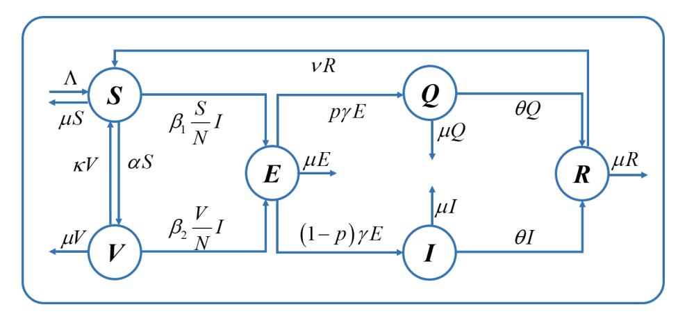
Figure 2: Transmission diagram of Covid-19 considering the compartments of vaccinated people and quarantined people.
Based on the diagram transmission in Figure 2, the formulation of the deterministic model is as follows
\[\frac{dS}{dt} = \Lambda - (\alpha + \mu)S - \beta_1 \frac{S}{N} I + \kappa V + \nu R,\] \[\frac{dV}{dt} = \alpha S - (\kappa + \mu)V - \beta_2 \frac{V}{N} I,\] \[\frac{dE}{dt} = \beta_1 \frac{S}{N} I + \beta_2 \frac{V}{N} I - (\gamma + \mu)E,\] \[\frac{dI}{dt} = (1 - p)\gamma E - (\theta + \mu)I,\] \[\frac{dQ}{dt} = p\gamma E - (\theta + \mu)Q,\] \[\frac{dR}{dt} = \theta(Q + I) - (\nu + \mu)R.\] (1)
System (1) is equipped with non-negative initial conditions, i.e., \(S(0) = S_0 \ge 0\), \(V(0) = V_0 \ge 0\), \(E(0) = S_0 \ge 0\)
\[E_0 \ge 0\], \(I(0) = I_0 \ge 0\), \(Q(0) = Q_0 \ge 0\), and \(R(0) = R_0 \ge 0\).
2.1. Positive Invariance
Since all variables of System (1) denote populations, then all of them must be non-negative for time \(t \ge 0\) when the initial conditions are also non-negative. Hence, it will be shown that System (1) is well-posed from a biological point of view. Considering the first equation in System (1), \(\frac{dS}{dt} \ge -\mu S\) for non-negative initial conditions. Therefore,
\[S(t) \ge S_0 e^{-\mu t} \ge 0. \tag{2}\]
This means that S(t) remains non-negative for all times t > 0. Analogous results hold for the other variables V(t), E(t), I(t), Q(t), and R(t).
The summation of all equations in System (1) yields a differential equation for the total population N(t) as follows
\[\frac{dN}{dt} = \Lambda - \mu N. \tag{3}\]
Solving equation (3) yields \(N(t) = \frac{\Lambda}{\mu} + (N(0) - \frac{\Lambda}{\mu})e^{-\mu t}\), where N(0) is the initial total population. As \(t \to \infty\), then \(N(t) \to \frac{\Lambda}{\mu}\). Hence, the feasible domain of System (1) is
\[\Omega = \left\{ (S, V, E, I, Q, R) \in \mathbb{R}_+^6 : 0 \le N \le \frac{\Lambda}{\mu} \right\},\tag{4}\] which is positively invariant. Thus, System (1) is well-posed.
2.2. The Basic Reproduction Number
System (1) has two equilibrium points, namely a disease-free equilibrium (DFE) given by \(X_0 = (\bar{S}, \bar{V}, 0, 0, 0, 0)\), where
\[\bar{S} = \frac{(\kappa + \mu)\Lambda}{\mu(\alpha + \kappa + \mu)}\] and \(\bar{V} = \frac{\alpha \Lambda}{\mu (\alpha + \kappa + \mu)}\)
and an endemic equilibrium \(X_1 = (S^*, V^*, E^*, I^*, Q^*, R^*)\) which will be discussed in Section (2.4).
The next-generation matrix method [11], [12] is applied to obtain an expression for the basic reproduction number of the System (1). In System (1), only the E and I compartments contribute to the appearance of new infections since it is assumed that quarantined individuals Q do not infect susceptible individuals. Linearization of the differential equations for the state variables E(t) and I(t) about the DFE \(X_0\) results in the Jacobian matrix
\[\mathbf{J} = \begin{pmatrix} -(\gamma + \mu) & \frac{\beta_1(\kappa + \mu) + \beta_2 \alpha}{\alpha + \kappa + \mu} \\ (1 - p) \gamma & -(\theta + \mu) \end{pmatrix}. \tag{5}\]
The Jacobian can be expressed as J = F - V [11] with
\[\mathbf{F} = \begin{pmatrix} 0 & \frac{\beta_1(\kappa + \mu) + \beta_2 \alpha}{\alpha + \kappa + \mu} \\ (1 - p) \gamma & 0 \end{pmatrix} \quad \text{and} \quad \mathbf{V} = \begin{pmatrix} \gamma + \mu & 0 \\ 0 & \theta + \mu \end{pmatrix}.\] (6)
The entries of \(\mathbf{F}\) correspond to the emergence of new infected individuals and the entries of \(\mathbf{V}\) correspond to all other state transitions [11], [12]. These matrices are used to compute the next-generation matrix as follows
\[\mathbf{NGM} = \mathbf{FV^{-1}} = \begin{pmatrix} 0 & \frac{\beta_1(\kappa + \mu) + \beta_2 \alpha}{(\alpha + \kappa + \mu)(\theta + \mu)} \\ \frac{(1-p)\gamma}{\gamma + \mu} & 0 \end{pmatrix}\] (7)
The basic reproduction number is defined as the spectral radius of the next-generation matrix, R0 = ρ(NGM) [11], [12]
\[\mathcal{R}_0 = \sqrt{\frac{\left[\beta_1(\kappa + \mu) + \beta_2 \alpha\right] (1 - p)\gamma}{(\theta + \mu)((\alpha + \kappa + \mu)(\gamma + \mu)}}.\] (8)
2.3. Stability of the Disease-free Equilibrium
If R0 < 1, then the unique disease-free equilibrium X0 of System (1) is locally asymptotically stable and if R0 > 1, then X0 is unstable.
Proof: The evaluation of the Jacobian matrix for (1) at X0 has eigenvalues −µ, −(µ + θ), −(µ + ν), −(µ + α + κ), and the roots of the polynomial
\[a_2\lambda^2 + a_1\lambda^2 + a_0 = 0, (9)\]
where
\[a_2 = \alpha + \kappa + \mu,\]
\[a_1 = (\alpha + \kappa + \mu)(\gamma + 2\mu + \theta),\]
\[a_0 = (\alpha + \kappa + \mu)(\gamma + \mu)(\theta + \mu)(1 - \mathcal{R}_0^2).\]
The characteristic polynomial (9) has two negative roots when R0 < 1. Thus, it is clear that X0 is locally asymptotically stable for R0 < 1 and unstable for R0 > 1.
2.4. Existence of a Unique Endemic Equilibrium
The unique endemic equilibrium point of System (1) is X1 = (S ∗ , V ∗ , E∗ , I∗ , Q∗ , R∗ ), with
\[S^{*} = \frac{(I^{*}\beta_{2}\mu + \Lambda \kappa + \Lambda \mu) (\gamma + \mu) (\mu + \theta) \Lambda}{\mu \gamma (1 - p) (I^{*}\beta_{1}\beta_{2}\mu + \Lambda \alpha \beta_{2} + \Lambda \kappa \beta_{1} + \Lambda \beta_{1}\mu)},\] \[V^{*} = \frac{(\gamma + \mu) (\mu + \theta) \Lambda^{2}\alpha}{\mu \gamma (1 - p) (I^{*}\beta_{1}\beta_{2}\mu + \Lambda \alpha \beta_{2} + \Lambda \kappa \beta_{1} + \Lambda \beta_{1}\mu)},\] \[E^{*} = \frac{I^{*} (\mu + \theta)}{(1 - p) \gamma}, \quad Q^{*} = \frac{I^{*}p}{1 - p}, \quad R^{*} = \frac{\theta I^{*}}{(1 - p) (\mu + \nu)},\] where I ∗ is defined implicitly by
\[\begin{split} f(I^*) = & b_2 I^{*2} + b_1 I^* + b_0, \\ b_2 = & \mu^2 \beta_1 \beta_2 \left( (\mu + \nu + \theta) \gamma + (\theta + \mu) (\mu + \nu) \right), \\ b_1 = & - (1 - p) \Lambda \gamma \mu \beta_1 \beta_2 (\mu + \nu) + \Lambda \mu \beta_2 (\theta + \mu) (\mu + \nu) (\gamma + \mu) \\ & + \Lambda \mu \left( \alpha \beta_2 + \kappa \beta_1 + \mu \beta_1 \right) \left( (\mu + \nu + \theta) \gamma + (\theta + \mu) (\mu + \nu) \right), \\ b_0 = & - \Lambda^2 (\mu + \gamma) (\mu + \alpha) (\mu + \theta) (\alpha + \kappa + \mu) (\mathcal{R}_0^2 - 1). \end{split}\]
According to Descartes' criterion, the polynomial f(I ∗ ) has one positive root (I ∗ > 0) since the sign of the coefficients of polynomial f(I ∗ ) change once, that is b2 > 0 and b0 < 0 when R0 > 1. Thus, X∗ is guaranteed to exist when R0 > 1. Figure 3 shows the bifurcation diagram of the equilibrium points with respect to β2, whereas other parameters are fixed. When the values of β2 for the case R0 < 1, X0 is asymptotically stable. Meanwhile, if the values of β2 in the case R0 > 1, X0 becomes unstable and a stable endemic equilibrium exists.
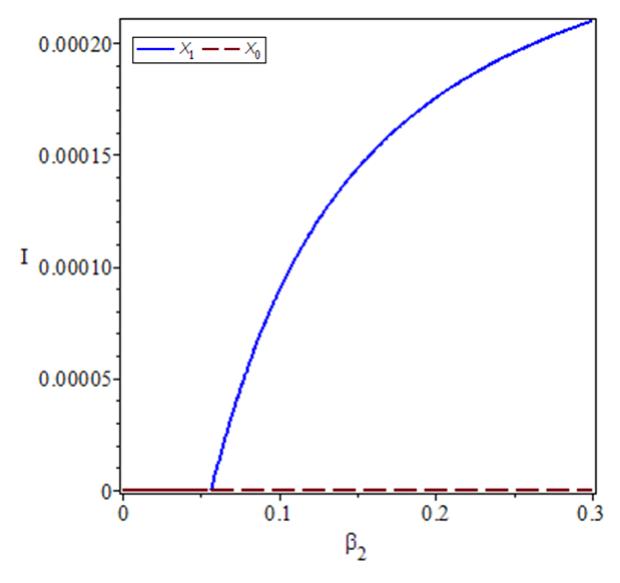
Figure 3: Bifurcation diagram of the equilibrium points with respect to parameter β2. Solid lines indicate the stable equilibriums and dashed lines indicate unstable equilibriums.
3. STOCHASTIC MODEL
3.1. Continuous-Time Markov Chain Model
In this section, we discuss a stochastic model for the spread of Covid-19 based on the deterministic model in Section 2. For convenience, the same notation used for the deterministic model is used in the stochastic model for the appropriate states. Let S(t), V (t), E(t), I(t), Q(t), and R(t) be discrete random variables representing the number of susceptible, vaccinated, exposed (infected but not yet infectious), infectious, quarantined, and recovered individuals after t ≥ 0 days, respectively. The related discrete-valued random vector is denoted as
\[X(t) = (S(t), V(t), E(t), I(t), Q(t), R(t)).\] (10)
A continuous-time Markov chain (CTMC) model is defined in terms of the state transitions that occur for the stochastic process {X(t)|t ∈ [0, ∞)} during an infinitesimally-small time period ∆t. The change ∆X(t) = X(t + ∆t) − X(t) has an infinitesimal transition probability r∆t + o(∆t). The state transitions and corresponding rates are summarized in Table 2.
3.2. Branching Process Approximation
To determine the probability of disease extinction, the nonlinear dynamics of the CTMC model are approximated near the DFE using a Galton-Watson multitype branching process as in [3], [4]. The only state variables contributing to the appearance of new infections are E and I. Therefore, the branching process approximation is only applied to these states, and the number of susceptible and vaccinated people is assumed to be close to disease-free equilibrium, S(t) ≈ S¯ and V (t) ≈ V¯ .
Both susceptible and vaccinated individuals can become infected through direct contact with infectious (non-quarantined) individuals. In the following, we use the term 'offspring' to describe susceptible or vaccinated people, each of whom was exposed through direct contact with an infectious person. The term 'offspring' will also be used for exposed people who develop an infectious state. We assume that the events associated with the infected states E(t) and I(t) are independent. That is, the number of offspring produced by a single exposed or infectious individual does not depend on the number of offspring produced by other exposed or infectious individuals. This assumption of independent events is the most restrictive leading to a Galton-Watson multitype branching process [3], [6], [18], [20].
| Description | Change | Rate, r |
|---|---|---|
| Recruitment | S → S + 1 | Λ |
| Rate of vaccination | (S, V ) → (S − 1, V + 1) | αS |
| Death of S | S → S − 1 | µS |
| Infection of S | (S, E) → (S − 1, E + 1) | β1SI/N |
| Death of V | V → V − 1 | µV |
| Infection of V | (V, E) → (V − 1, E + 1) | β2V I/N |
| V becomes S | (V, S) → (V − 1, S + 1) | κV |
| Exposed to infectious | (E, I) → (E − 1, I + 1) | (1 − p)γE |
| Exposed to quarantined | (E, Q) → (E − 1, Q + 1) | pγE |
| Death of E | E → E − 1 | µE |
| Recovery of I | (I, R) → (I − 1, R + 1) | θI |
| Death of I | I → I − 1 | µI |
| Recovery of Q | (Q, R) → (Q − 1, R + 1) | θQ |
| Death of Q | Q → Q − 1 | µQ |
| Loss of immunity | (R, S) → (R − 1, S + 1) | νR |
| Death of R | R → R − 1 | µR |
Table 2: State transitions and corresponding rates describing the CTMC model.
The probability of disease extinction is defined as
\[P_0 = \lim_{t \to \infty} \text{Prob}\{E(t) + I(t) = 0\}.\] (11)
Note that the probability of disease extinction does not depend on the number of quarantined individuals Q(t) since it is assumed quarantined individuals are not capable of infecting susceptible individuals. Thus, even if infectious quarantined individuals are present, they will eventually recover or die without transmitting the disease producing new infections. An expression for the probability of disease extinction can be obtained from the offspring probability generating functions (pgfs) for the states E and I.
In general, for xi(0) = 1 and xj (0) = 0 where j ̸= i, the offspring probability generating function (pgf) for individuals of type i is the function fi : [0, 1]n → [0, 1]n defined by
\[f_i(x_1, \dots, x_n) = \sum_{k_1=1}^{\infty} \dots \sum_{k_n=1}^{\infty} P_i(k_1, \dots, k_n) x_1^{k_1} \dots x_n^{k_n},\] (12)
where Pi(k1, . . . , kn) denotes the probability that one type i individual gives 'birth' to kj individuals of type j [3], [4]. For the branching process approximation, we consider exposed people as type 1 individuals (x1), and infected people as type 2 individuals (x2).
The offspring pgf for E, given E(0) = 1 and I(0) = 0, is
\[f_1(x_1, x_2) = \frac{(1-p)\gamma x_2 + p\gamma + \mu}{\gamma + \mu}.\] (13)
The term (1 − p)γ/(γ + µ) is the probability that a person changes status from exposed to infectious (nonquarantined), the term pγ/(γ+µ) is the probability that a person changes status from exposed to quarantined, and the term µ/(γ + µ) is the probability of natural death for an exposed person before becoming infectious or quarantined.
The offspring pgf for I, given E(0) = 0 and I(0) = 1, is
\[f_2(x_1, x_2) = \frac{\beta_1(\kappa + \mu)x_1x_2 + \beta_2\alpha x_1x_2 + (\theta + \mu)(\alpha + \kappa + \mu)}{\beta_1(\kappa + \mu) + \beta_2\alpha + (\theta + \mu)(\alpha + \kappa + \mu)}.\] (14)
The term β1(κ+µ)/(β1(κ+µ)+β2α+(θ+µ)(α+κ+µ)) is the probability that a susceptible person becomes exposed as a result of contact with an infectious person. The term β2α/(β1(κ+µ)+β2α+(θ+µ)(α+κ+µ)) is the probability that a vaccinated person becomes exposed as a result of contact with an infectious person.
The term \((\theta + \mu)(\alpha + \kappa + \mu)/(\beta_1(\kappa + \mu) + \beta_2\alpha + (\theta + \mu)(\alpha + \kappa + \mu))\) is the probability of recovery or death of an infected person.
The expectation matrix \(M = [m_{ij}]\) is a non-negative \(2 \times 2\) matrix, whose entries are defined as
\[m_{ij} = \frac{\partial f_j}{\partial x_i},\tag{15}\] where the partial derivatives are evaluated at the fixed point \((x_1, x_2) = (1, 1)\) [3], [4]. The entry \(m_{ij}\) denotes the expected number of type i offspring produced by one individual of type j. The expectation matrix \(M = [m_{ij}]\) for the offspring pgfs is
\[M = \begin{pmatrix} 0 & \frac{\beta_1(\kappa + \mu) + \beta_2 \alpha}{\beta_1(\kappa + \mu) + \beta_2 \alpha + (\theta + \mu)(\alpha + \kappa + \mu)} \\ \frac{(1 - p)\gamma}{\gamma + \mu} & \frac{\beta_1(\kappa + \mu) + \beta_2 \alpha}{\beta_1(\kappa + \mu) + \beta_2 \alpha + (\theta + \mu)(\alpha + \kappa + \mu)} \end{pmatrix}\](16)
Since the expectation matrix M is irreducible and the offspring pgfs \(f_i\) are non-singular, there are at most two fixed points \((x_1,x_2)\in[0,1]^2\) [26]. If the process is subcritical or critical \((\rho(M)<1\) or \(\rho(M)=1\)), then the point (1,1) is the only fixed point. However, if the process is supercritical \((\rho(M)>1)\), then there is a unique second fixed point \((q_1,q_2)\in(0,1)^2\) of the offspring pgfs [18], [26]. The probability of disease extinction is calculated using the fixed point \((q_1,q_2)\in(0,1)^2\). In particular, the probability of disease extinction is
\[P_0 = \begin{cases} 1 & \text{if } \rho(M) \le 1, \\ q_1^{E(0)} q_2^{I(0)} & \text{if } \rho(M) > 1. \end{cases}\] (17)
Thus, the spectral radius of the expectation matrix \(\rho(M)\) serves as a threshold for disease persistence or extinction for the stochastic model in the same way that the basic reproduction number \(\mathcal{R}_0\) is a threshold for the deterministic model [3], [4]. The spectral radius of M is given by
\[\rho(M) = \frac{1}{2} \left[ A + \sqrt{A^2 + 4AB} \right],\tag{18}\] where
\[A = \frac{\beta_1(\kappa + \mu) + \beta_2 \alpha}{\beta_1(\kappa + \mu) + \beta_2 \alpha + (\theta + \mu)(\alpha + \kappa + \mu)},\]
\[B = \frac{(1 - p)\gamma}{\gamma + \mu}\]
The Threshold Theorem in [4] gives the following relationship between \(\rho(M)\) and \(\mathcal{R}_0\):
\[\mathcal{R}_0 < 1 \ (=1, >1) \iff \rho(M) < 1 \ (=1, >1).\] (19)
The hypotheses of the Threshold Theorem are satisfied since the matrix F in (6) is non-negative, the expectation matrix M is irreducible, and the matrix V in (6) is a non-singular M-matrix.
Let \(E(0) = e_0\) and \(I(0) = i_0\) for \(\mathcal{R}_0 > 1\), then the probability of extinction of disease define
\[P_0 = \lim_{t \to \infty} \text{Prob}\{E(t) + I(t) = 0\} = q_1^{e_0} q_2^{i_0}, \tag{20}\]
for the unique fixed point \((q_1, q_2) \in (0, 1)^2\) of the offspring probability generating functions. The values of \(q_1\) and \(q_2\) are given by
\[q_{1} = \frac{p\gamma + \mu}{\gamma + \mu} + \frac{(1-p)\gamma}{\gamma + \mu} \frac{1}{\mathcal{R}_{0}^{2}},\] \[q_{2} = \frac{1}{\mathcal{R}_{0}^{2}},\] (21)
Here, the term \(q_1\) denotes the probability of disease extinction for a single exposed individual. Meanwhile, the term \(q_2\) is the probability of disease extinction for a single infectious (non-quarantined) individual. The expressions for \(q_1\) and \(q_2\) can be interpreted epidemiologically. Given one exposed individual, either that individual dies from natural causes with probability \(\mu/(\gamma+\mu)\), survives and progresses to a quarantined status with probability \(p\gamma/(\gamma+\mu)\), or survives and progresses to an infectious (non-quarantined) status with probability \((1-p)\gamma/(\gamma+\mu)\). Then the infectious individual succesfully transmits the infection with probability \(q_1=1/\mathcal{R}_0^2\). Note that \(q_2< q_1\) which is biologically reasonable since the disease is more likely to persist if individuals are already infectious rather than only exposed to the disease.
4. NUMERICAL ANALYSIS
In this section, we perform numerical simulation of the deterministic and stochastic models as well as sensitivity analysis of \(\mathcal{R}_0\), \(P_0\), and the equilibrium values with respect to the model parameters. All simulations use the parameter values in Table 3.
| Symbol | Parameter | Value | Unit | References |
|---|---|---|---|---|
| Λ | Recruitment rate | \(N\mu\) | human/day | assumed |
| \(\mu\) | Death rate | \(1/(70 \times 365)\) | human/day | assumed |
| \(\alpha\) | Vaccination rate | \(1.10^{-4} - 4.2.10^{-3}\) | 1/day | [25] |
| \(\kappa\) | The reduction rates of antibodies by vaccination | 1/240 - 1/180 | 1/day | [10] |
| \(\beta_1\) | Infection rate of S | 0.119 - 0.282 | - | [32] |
| \(\beta_2\) | Infection rate of V | 0.05 - 0.2 | - | assumed |
| p | Proportion of quarantined humans E | 0 - 1 | - | assumed |
| \(\gamma\) | Latency period | 1/5.5 | 1/day | [14] |
| \(\theta\) | Recovery rate | 1/10 | 1/day | [14] |
| \(\nu\) | The reduction rates of antibodies by natural infection | 1/240 - 1/180 | 1/day | [10] |
Table 3: Parameter values with their description used in the simulation.
Figure 4 shows the plots of one sample path of the CTMC model and the solution of deterministic model with \(\alpha=0.0001,\ p=0.45,\ \beta_1=0.25,\ \beta_2=0.1,\ \kappa=\nu=1/210,\) and \(\mathcal{R}_0=1.1651.\) It can be seen that for the SVEQIR model with loss of immunity to V and R after a certain period of time, there will be an epidemic in the long term.
4.1. Level Sets \(\mathcal{R}_0\)
The level sets of \(\mathcal{R}_0\) for some parameters are given in Figure 5. Figures 5(a) and 5(d) show that the values of \(\beta_2\) and \(\kappa\) are proportional to the value of \(\mathcal{R}_0\), while the value of \(\alpha\) is inversely proportional to the value of \(\mathcal{R}_0\). These results provide knowledge that the value of \(\mathcal{R}_0\) can be reduced by using a vaccine with higher efficacy (decreasing \(\beta_2\)) and a longer effective period (decreasing \(\kappa\)). Furthermore, Figures 5(b) and 5(c) show that increasing p or \(\alpha\) decreases the value of \(\mathcal{R}_0\). These results indicate that the value of \(\mathcal{R}_0\) can be reduced by increasing the proportion of people who are quarantined and the proportion of people who are vaccinated.
4.2. Sensitivity Index of \(\mathcal{R}_0\)
We analyzed the sensitivity of \(\mathcal{R}_0\) to model parameters using a normalized forward sensitivity index as defined in [7]. In particular, the forward sensitivity index of the normalized variable u, which depends on the parameter p, is defined as
\[\Upsilon_p^u = \frac{\partial u}{\partial p} \times \frac{p}{u}.\] (22)
The sensitivity index of \(\mathcal{R}_0\) can be calculated for each model parameter given in Table 3. Using the parameter values given in Table 3, the sensitivity index \(\mathcal{R}_0\) to the parameters in System (1) is evaluated using equation (22) and the results are given in Table 4.
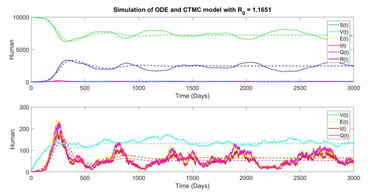
Figure 4: Simulation of ODE (dashed) and CTMC (solid) models with α = 0.0001, p = 0.45, β1 = 0.25, β2 = 0.1, κ = ν = 1/210, and R0 = 1.1651.
| Scenario 1 | Scenario 2 | |||||
| R0 = 1.1651 | R0 = 1.2724 | |||||
| (α, p) = (0.0001, 0.45) | (α, p) = (0.0042, 0.1) | |||||
| Parameter (p) | Sentivity index (ΥR0 ) p | Parameter (p) | Sentivity index (ΥR0 ) p | |||
| 1 | θ | -0.4998 | 1 | θ | -0.4998 | |
| 2 | β1 | +0.4959 | 2 | β1 | +0.3704 | |
| 3 | p | -0.4091 | 3 | β2 | +0.1296 | |
| 4 | α | -0.0061 | 4 | α | -0.1037 | |
| 5 | κ | +0.0060 | 5 | κ | +0.1029 | |
| 6 | β2 | +0.0041 | 6 | p | -0.0556 | |
| 7 | µ | -0.0003 | 7 | µ | +0.0005 | |
| 8 | γ | +0.0001 | 8 | γ | +0.0001 | |
| 9 | ν | 0 | 9 | ν | 0 | |
Table 4: Sensitivity indices of R0 to parameters.
Table 4 shows the sensitivity indices of R0 for two scenarios of pairs α and p. From the table, it can be observed that the level of antibody reduction by natural infection (ν) has no effect on R0. This occurs because the expression for R0 does not contain ν. The basic reproduction number R0 is the most sensitive to the recovery rate (θ) and the infection rate of S by I (β1), respectively. Meanwhile, R0 is the least sensitive to the latency period (γ) and the natural death rate (µ), respectively. However, these four parameters are not easy to control through human intervention. Thus, we pay our attention to other parameters, namely p, α, κ, and β2. These parameters have different sensitivity orders in Scenarios 1 and 2, depending on the magnitude of each value. The value of R0 in Scenario 1 is closer to the situation in Indonesia. Under Scenario 1, R0 is more sensitive to the parameter p, followed by α, κ, and β2. This is in accordance to the level set of R0 in the previous subsection. Figure 5(b) that showed the level set of R0 to p and α has the longest interval of R0 compared to three other figures. Under this circumstance, since the current vaccines do not give full protection and the antibodies from vaccination has limited time, it is still necessary to quarantine the infected.
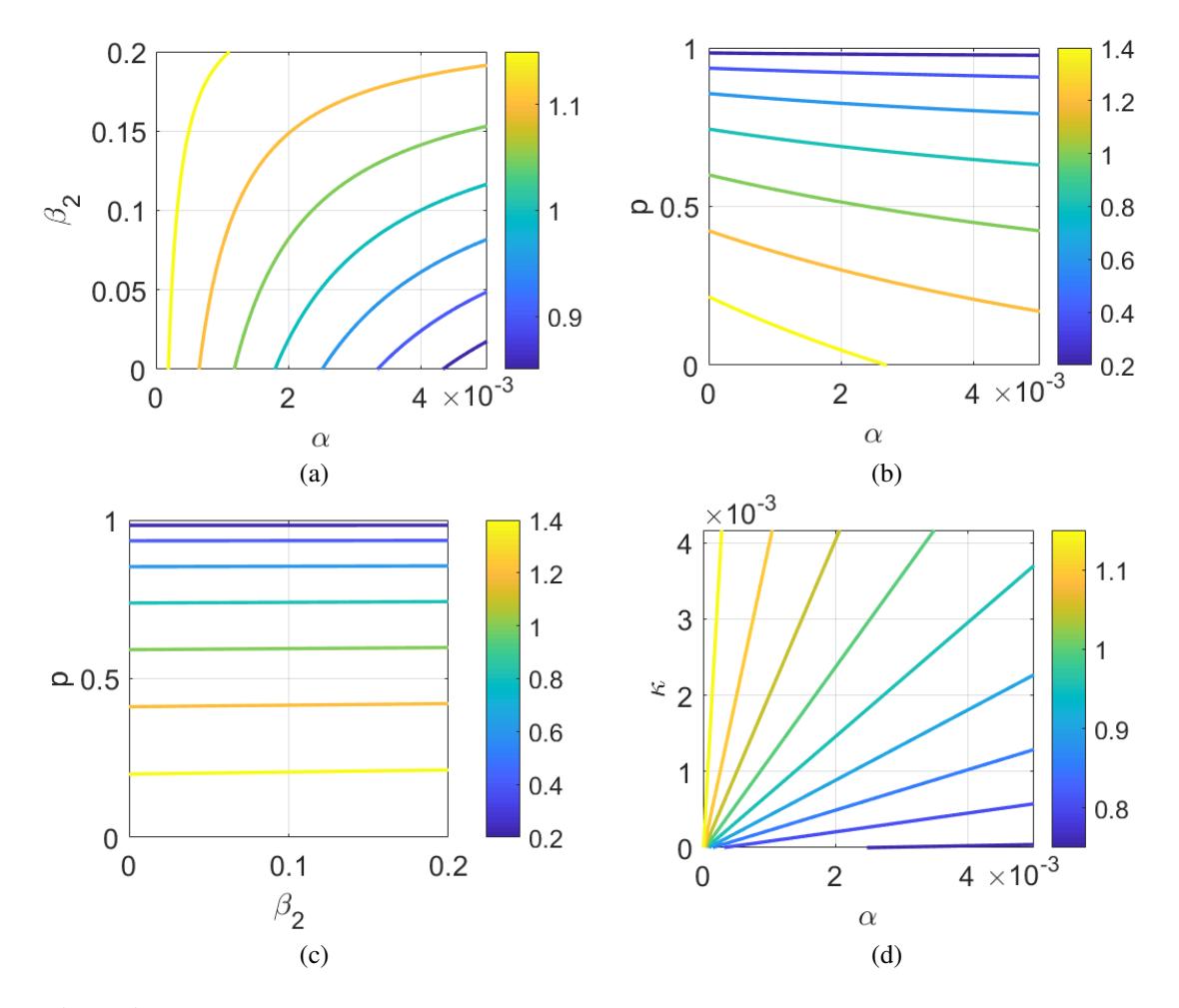
Figure 5: Level set of R0 with data in Table 3: α = 0.0001, p = 0.45, β1 = 0.25, β2 = 0.1, κ = ν = 1/210.
4.3. Probability of Disease Extinction
The expression q1 in equation (21) represents the probability of extinction of the disease in the state E, and the expression q2 represents the probability of extinction in the state I. In Figure 6, the sensitivity of each quantity is shown in relation to vaccination rate, infection rate, and proportion of quarantined individuals. Figure 6 shows that the values of α and p are directly proportional to q1 and q2, while values of β2 are inversely proportional to q1 and q2. These results indicate that increasing the vaccine's efficacy, the rate of vaccination, and the proportion of quarantined infected people contributes to improving the probability of extinction of Covid-19 in the population.
The probability of disease extinction P0 is calculated for several sets of initial conditions using the equation (20). This probability is compared with the numerical estimate (Approx.) of disease extinction in the CTMC model simulation. The numerical estimations are obtained from the proportion of 10,000 sample paths of the CTMC for which disease extinction occurs (E(t) = I(t) = 0) before time t = 320, which is the peak of the deterministic model. The results are summarized in Table 5 with parameter values as in Table 3 and initial conditions S(0) = 30, 000 − E(0) − I(0), V (0) = 0, E(0), I(0), Q(0) = 0, and R(0) = 0.
In Table 5 it can be seen that the analytical value of the probability of extinction is very close to the estimated extinction value obtained from the 10,000 sample simulation. This shows that the probability of disease extinction can be calculated by the formula obtained P0 (21). Meanwhile, for the simulation case in
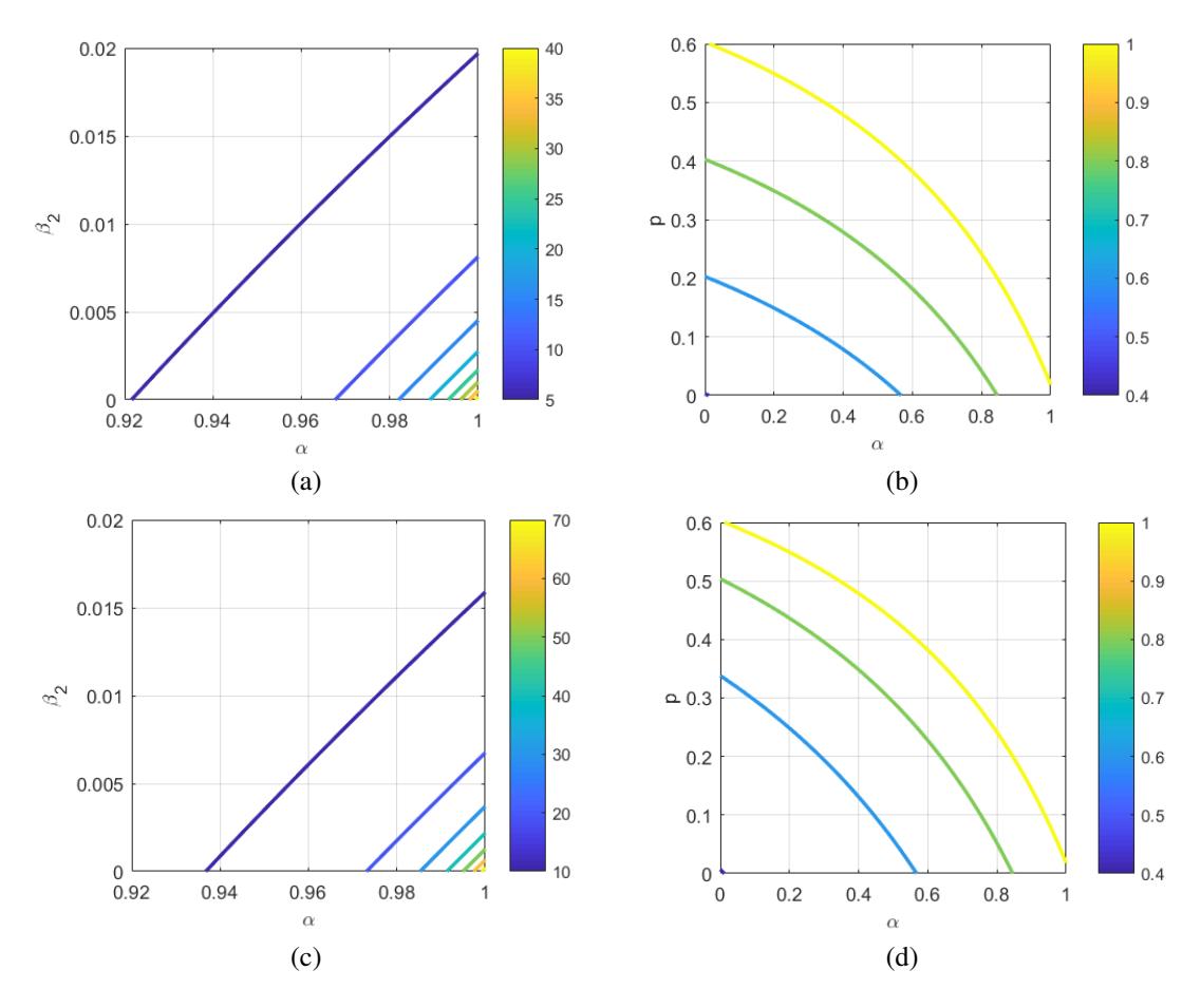
Figure 6: Level set of q1 (a) and (b), and level set of q2 (c) and (d) by using the data in Table 3: α = 0.0001, p = 0.45, β1 = 0.25, β2 = 0.1, κ = ν = 1/210.
Table 5: An analytical calculation of the probability of disease extinction P0 and its numerical approximation (Approx.) based on 10,000 sample paths of the CTMC model.
| E(0) | I(0) | R0 | P0 | Approx. |
|---|---|---|---|---|
| 1 | 0 | 1.1651 | 0.8552 | 0.8545 |
| 2 | 0 | 1.1651 | 0.7314 | 0.7316 |
| 0 | 1 | 1.1651 | 0.7367 | 0.7381 |
| 0 | 2 | 1.1651 | 0.5428 | 0.5493 |
| 1 | 1 | 1.1651 | 0.6301 | 0.6256 |
| 1 | 2 | 1.1651 | 0.4642 | 0.4565 |
| 2 | 1 | 1.1651 | 0.5389 | 0.5320 |
| 2 | 2 | 1.1651 | 0.3970 | 0.3990 |
Figure 4, for a very long time (t = 3000 days), the values obtained are I(3000) ≈ 65 and E(3000) ≈ 65. This result gives the value P0 = 1.36 × 10⁻¹⁴ ≈ 0 where R0 = 1.1651. This is in accordance with the solution plots in Figure 4, where there will be an epidemic for a long time.
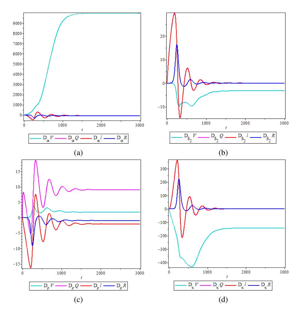
Figure 7: Sensitivity analysis of V, Q, I, and R with respect to parameters \(\alpha\), \(\beta_2\), p, and \(\kappa\) with data in Table 3.
4.4. Sensitivity Analysis of Variables
Next, we analyze the sensitivity of solutions of System (1) to changes in the model parameters. There are six variables and nine parameters which yield 54 sensitivity analysis simulations. The sensitivity simulation is obtained by the following procedure. Rewriting System (1) as \(X_t = G(X, \mathbf{p})\) with \(X_t = \frac{dX}{dt}\), \(\mathbf{p} = (\alpha, \beta_1, \beta_2, p, \gamma, \theta, \mu, \kappa, \nu)^T\) and \(X(t) = (S(t), V(t), E(t), I(t), Q(t), R(t))^T\). The notation \(\partial_p X\) represents the change of solution X(t) to the change of parameter p [29], [21].
Let \(K = \partial_p X\) and assume that K is differentiable, then the derivative of K to time t can be obtained by using the chain rule as follows
\[\partial_t K = \partial_p G(X, p) = \partial_X G \,\partial_p X + \partial_p X,\tag{23}\] so that
\[\partial_t K = (\partial_X G)K + \partial_p G. \tag{24}\]
Equation (24) is a dynamical system with \(\partial_X G\) and \(\partial_p G\) are \(6 \times 6\) Jacobian matrix and \(6 \times 9\) matrix, respectively. Since the system yields 54 sensitivity simulations, then we only focus on variables V, Q, I, and R along with the fluctuating parameters due to human interventions or public policies such as \(\alpha, \beta_2\), p, and κ. Furthermore, a sensitivity analysis around the non-explicit endemic equilibrium (10) is simulated based on the values of the parameters in Table 3, as shown in Figure 7.
Values in Figure 7 represent the sensitivity of variables for the corresponding parameters, whereas the signs (positive or negative) denote the relation of direction. Hence, from Figure 7, we observe that V , Q, I and R are the most sensitive to α, κ, and followed by β2 and p, even to β2 and κ. Figures 7(a) and (c) show that variable V is directly proportional to α and p, but two other figures show it is inversely proportional to β2 and κ. Meanwhile, the direction change of variables Q, I and R fluctuate at the beginning of time, but after t = 1500 they show almost no more change. This means that the endemic equilibrium has been reached. Furthermore, from the magnitude of the change of variables to time t in Figure 7(b) and (c) show that parameters β2 and p just make a slight change to all variables. However, V is much more sensitive to α compared to other parameters and even other variables to that parameter. Therefore, increasing the vaccinated people and extending the antibodies resistance due to vaccines will reduce the number of the infected.
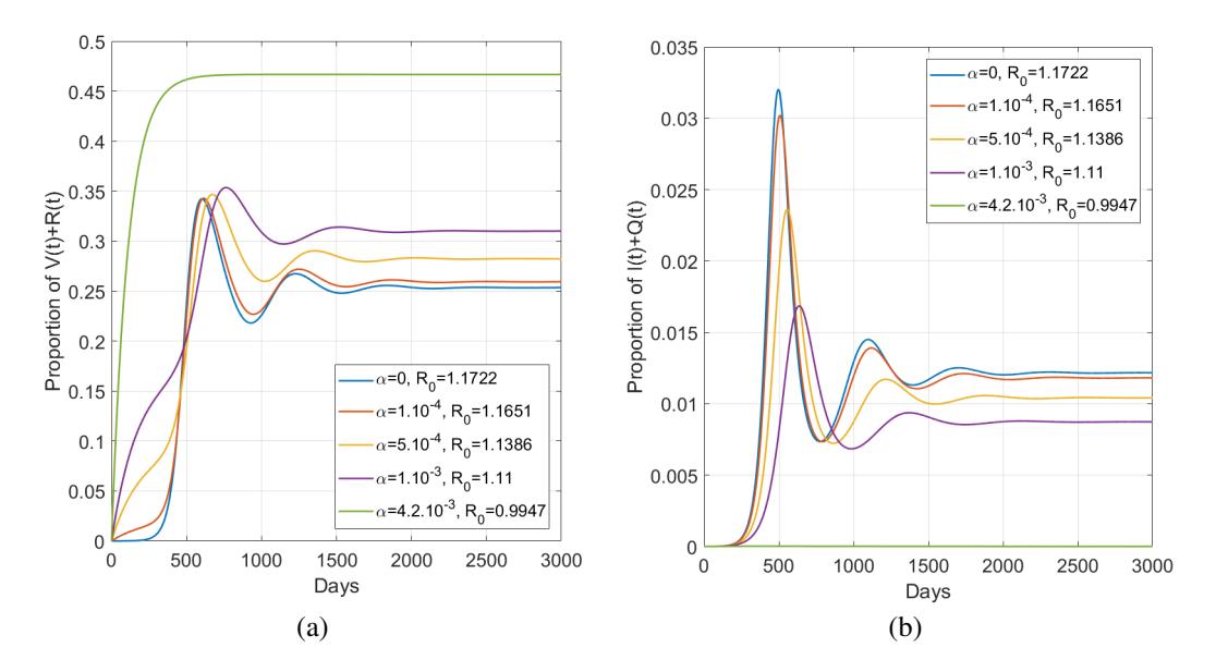
Figure 8: The proportions of V (t) + R(t) and I(t) + Q(t) with different α.
The current study states that herd immunity in Indonesia will be achieved if the proportion of the population that has immunity is about 70% [13], [1]. In this model, we assume that the number of humans who have immunity is the total population of V (t)+R(t). Figure 8 shows the proportions of V (t)+R(t) and I(t)+Q(t) in a population with several different α scenarios. In Figure 8, it can be seen that the average vaccination rate has a significant effect on increasing the proportion of the population who has immunity. However, for possible scenarios on average vaccine administration based on [25], herd immunity has not been achieved in Indonesia.
The next important factor is β2, which is the infection rate of people who have been vaccinated. The greater the value of β2, the lower the vaccine efficacy. Figure 9 shows the proportions of V (t) + R(t) and I(t) + Q(t) in a population with several scenarios of β2. From Figure 9, it can be said that the lower the vaccine efficacy, the lower the amount V (t) + R(t) and the higher the amount I(t) + Q(t) . Thus, it can be concluded that the use of vaccines with higher efficacy can be applied as an effort to reduce the number of infected humans.
Considering the two most influential factors in the vaccinated compartment, namely the vaccination rate and the infection rate in the vaccinated compartment, we simulated several scenarios of the pairs of (α, β2). Figure 10 shows the simulation results in the proportion of the number of compartments V (t) + R(t) and I(t)+Q(t) for the scenarios of the highest and lowest rate combinations at the values α and β2, respectively. From the simulation, it can be seen that the effect of the value of α is greater than the effect of the value of
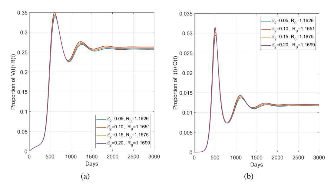
Figure 9: The proportions of V (t) + R(t) and I(t) + Q(t) with different β2.
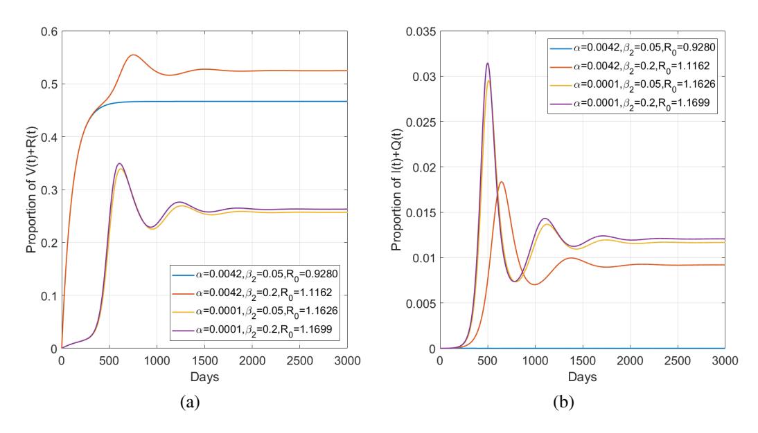
Figure 10: The proportions of V (t) + R(t) and I(t) + Q(t) with different pairs of (α, β2).
β2 for each proportion. That is to say, the speed of administration of the vaccine is more influential than the efficacy of the vaccine to increase the number of populations that have immunity and reduce the number of infected people.
Figure 11 shows a simulation of several scenarios for the pairs of (α, p). The proportion of I(t) + Q(t) is always proportional to R0 as shown in Figure 11(b), while the proportion of V (t) + R(t) is not always proportional to R0 as shown in Figure 11(a). However, it can be observed that for the same value of p, the greater the value of α, the greater the proportion of V (t)+R(t). Meanwhile, for the same α value, the greater
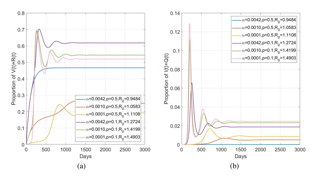
Figure 11: The proportions of V (t) + R(t) and I(t) + Q(t) with different pairs of (α, p).
the value of p, the lower the value of V (t) + R(t). It can be explained by the parameter p (proportion of people quarantined) which is indirectly inversely proportional to the proportion of R(t), while the parameter α (vaccination rate) is proportional to the proportion of V (t).
5. CONCLUSION
In this study, we considered an extended SEIR model of Covid-19 transmission with the addition of vaccinated and quarantined compartments. Thus, the rate of vaccination, the efficacy of the vaccine used, and the proportion of the number of infected people who were quarantined became control parameters. We analyzed some important indicators for disease transmission through deterministic and stochastic models, namely the basic reproduction number and the probability of extinction of Covid-19. Numerical simulations were performed for the deterministic and stochastic models reflecting the epidemic in Indonesia. The results of this study lead to two main recommendations for dealing with the Covid-19 epidemic in Indonesia. First, increasing the proportion of humans who are vaccinated to reduce the possibility of people being infected when coming into contact with an infected person. Second, since the current vaccines do not provide full protection and their efficacy only lasts for a limited time, quarantining infected people is still necessary to reduce the proportion of infectious individuals transmitting the disease. The efforts to increase the rate of vaccination can be done by increasing the average daily administration of vaccines in Indonesia. On the other hand, the limitations of the Indonesian government on distributing the vaccine can be offset by implementing a quarantine program for infected people. The quarantine does not have an impact on increasing the number of people who are immune directly, but it can reduce the number of people who can transmit the disease. Additionally, an important parameter for reducing the number of infected people is the efficacy of the vaccine itself. We believe that this study provides some insights in understanding the transmission of Covid-19 with the vaccination program, although this model is limited by some assumptions.
ACKNOWLEDGEMENT
This research was supported by the Simlibtabmas of Indonesian Education Scholarship Program, Ministry of Finance and Research, Technology, and Higher Education of the Republic of Indonesia.