

1. Introduction
Now a days, the world is burden with infectious diseases throughout the world and these diseases have a great influence on the human population. The history referrers that plague [1], Nipah [2], [3], swine flu [4], hepatitis B [5], [6], HIV/AIDS [7]–[10], TB [11], COVID-19 [12]–[14] etc. are most dangerous infectious diseases that cause a huge loss of human life. From its very beginning scientists have been trying to control these kinds of fatal diseases. After the manifestation of any infectious virus, it starts to increase very fast sensibly or insensibly and people need the effective method to resist the outbreak of the disease or at least to control the number of infections [12], [15]. Transmission diseases have ever been a great concern of human being from the very beginning of our history and HIV/ AIDS and TB are two of them. The primary and the second infectious causes of mortality are marked from the human immunodeficiency virus (HIV) and mycobacterium tuberculosis [16]. AIDS is an HIV-related illness spread mostly by unprotected sexual contact, infected blood transfusions, hypodermic needles, and transmission from mother to child during pregnancy, childbirth, or feeding [17], [18].
Millions of people die annually from tuberculosis and HIV/ AIDS and billions of others are being infected. AIDS is an extremely hazardous illness that may be found practically anywhere in human civilization. However, it has not had an equal impact on all civilizations throughout the world. People with AIDS are constantly at risk of death, and HIV is the cause of the disease. HIV is a dangerous virus that renders the human body almost incapable of combating diseases. The HIV virus gradually destroys the human immune system by causing a reduction in CD4+T cell numbers [17], [19]. Significant immunological damage aids the development of opportunistic processes, allowing infections to begin in the body. The immune system, like the digestive system, is significantly reliant on our bodies to combat illnesses and digest food. Some forms
*Corresponding author of infections are also prevented by the immune system in the body. A person will have to die even from a mild virus like a cold or flu if their immune system is completely decimated [8], [9], [20]. Tuberculosis more commonly known as TB is a bacterial infectious disease which can co-infect with HIV. TB can be seen as latent (inactive) or active [21]. Dormant or latent tuberculosis affects about a third of the world's population [20]. People living with TB gradually loss the immune system and as a result it causes a great health hazard. TB and the HIV have a complicated interaction. The HIV and TB co-infection can spread out at an individual and community level [58]. Human immunodeficiency virus (HIV) and Tuberculosis (TB) jointly become the serious global mass health challenge. The incarnation of AIDS makes the relation between HIV and TB. HIV and tuberculosis co-infection occurs when an individual is HIV positive and is either exposed to or infected with tuberculosis. Infection with tuberculosis germs is not a given for HIVpositive people. Individuals infected with tuberculosis do not inevitably get HIV until they come into contact with HIV-positive people [22]. AIDS/HIV and tuberculosis remain the world's most deadly epidemics and major infectious killer diseases, with the afflicted patient's ultimate fate being early death [23].
There are so many ways to mould the biological system into modeling, to solve the system and to make the decisions of complex diseases models. In these cases, optimal control policies of diseases are widely used to prevent the outbreak of infections. Control theory deals with systems that can be controlled whose evolution influenced by some external agents. It is a method for determining control and state trajectories for a dynamical system over time in order to optimize a performance index [5]. Sometimes two or more strategies are applied to find the better one to minimize the spreading of virus as well as the cost of the treatment. For instances Awoke and Kassa [24] used the theory of control to solve the entire model with the goal of lowering the total cost of infections and control efforts. Gupta et al. [25] used control as first and second line of treatment. Fatmawati and Tasman [26] considered optimal anti-TB Treatment and antiretroviral as control to control the TB and HIV. Biswas [27], [28] represented a simple SEIR model showing the application of optimal control to reduce infection with and without state constraints. Moreover, there are so many extensive researches [29]–[31] about the applications of optimal control strategies to develop the mathematical model of TB and HIV/AIDS control among the general mass. The bookworms, researchers and general readers are suggested to follow some papers for more information about HIV-TB as well as other infectious diseases with developments of mathematical modeling and optimal control strategies. Azim et al. [32] discuss current, past and possible future scenarios of HIV in Bangladesh. Also male, female, sexual and age wise data are shown in the paper. Biswas, Paiva and Pinho [8], [27], [28] analyzed a model deal with the evolution of HIV/AIDS and their optimal control. They also discussed a SEIR model with their constraints. Constantinos et al. [33] worked with the dynamics of infectious disease. Islam et. al. [34] analyzed and discussed about the very recent pandemic disease called COVID-19 that have killed about 4.5 million people already. Khatun and Biswas [35] worked with the leukemia mostly known as blood cell disease and applied control policy to minimize the disease. Mahmud [20] discussed about the Tuberculosis and HIV, their infection in Bangladesh. Silva et al. [16] deal with the coinfection model and show how to apply treatment in coinfection model. Zaman et al. [36], [37] represented and analyzed TB data and showed the severity of TB worldwide. Zumla et al [38] showed how human can be attacked by the HIV after the TB has weakened the immune system.
Felling the severity of HIV/AIDS and TB worldwide as well as in Bangladesh, we are intended to do the work about it in this paper. However, describing the epidemiology of these infectious diseases and adopting any control strategy is not an easy task. By using mathematical modeling, we analyze the transmission and disease behaviors of epidemiological models. For the prevention and mitigation of disease transmission, we employ two control variables. The numerical computation is done by us of this model by using ODE45solver in MATLAB programming language. The following is an overview of the paper's structure: In section 1 we discussed the introduction of this paper. The model is formulated in section 2. We mathematically explain the existence of state variables in section 3 and objective functional in section 4. We discussed the basic reproduction ratio and optimal control in section 5 as well as applied Pontryagin's maximum principle to drive the results. In section 6, numerical simulations and discussion of the accompanying HIV/AIDS-TB model's outcomes are carried out. The paper is ended with conclusion and possible future works.
2. MODEL FORMULATION AND BASIC PROPERTIES
There are 10 compartments in the total population model that are Susceptible individuals S Latent TB with no HIV LT , Exposed to TB only ET0, Symptomatic TB ST , Infected with HIV only IH, Those who have recover with temporal immunity RT , individuals infected with HIV (pre-AIDS) exposed to TB ETH,
HIV infected displaying AIDS symptoms HS, AIDS individuals exposed to TB EHT and AIDS individuals dually infected with TB HDT . We suppose that susceptible individuals are recruited at a per capita rate of A into the population. Individuals in the classes HS and EHT die due to TB at the rate d1 and die to AIDS at a rate d2 assuming that it is difficult to identify the cause of deaths in these classes. Susceptible people get HIV when they come into touch with HIV-positive people at rate λ1, and when they come into touch with an infected individual at rate λ2, they get TB. It is supposed that all individuals in various subgroups die naturally at a constant rate µ. Individuals may get natural recovery from TB and then enter into the recovery class at a constant rate r1 and relapsing rate for the individuals with symptom of TB is r2. We assume that κ1 ≤ κ2 where κ1 is the TB propagation rate infected with AIDS and κ2 is the HIV infected rate with Mtb progress to AIDS. Bhunu et al. [29] found force of infection in their calculation for HIV infection and in light of their work the force of infection associated with HIV infection in our model [29] is given by,
\[\lambda_1 = \frac{\beta_1}{N} (I_H + E_{TH}) + \eta_2 (H_S + \eta_1 (\eta_3 H_{DT} + E_{TH}))]. \tag{1}\]
Here β1 is considered as the effective contract rate of HIV infection. In the AIDS stages infected individuals have relative effectiveness with HIV, that is called modification parameter, η1 ≥ 1. The parameter η2 ≥ 1 shows the fact that individuals who are in the AIDS stage of infection are more infectious than HIV infected individuals with no AIDS symptoms. The rate η3 ≥ 1 indicates that dually infected individuals in the AIDS stage show symptom of TB are considered more infectious than the individuals who are only exposed to TB. The parameter c ≥ 1 shows the number of contacts having only HIV and no TB where the rate indicates number of contacts having HIV and TB. Similarly the force of infection associated with TB infection is given by,
\[\lambda_2 = \frac{\beta_2 c}{N} (S_T + H_{DT}),\tag{2}\] where β2 is the probability that one individual being infected with one infectious individual and c is per capita contact rate. The rate of progression to AIDS is assumed to ρ1. Individuals who are exposed to TB in the AIDS stage of HIV infection are getting active TB at a constant rate κ3. ψ2λ2 is the rate at which the individuals get his own development with TB and ψ3λ2 is the rate at which the individuals get his own development with symptom of TB with ψ2 > 1. There are some non liner term used in the model as unpredictable interactions occur in different stages of HIV/AIDS and TB co-infection that rein in the system under consideration [39]. At a time t the total population size N(t) is written as,
\[N(t) = S(t) + L_T(t) + I_H(t) + H_S(t) + E_{TH}(t) + E_{HT}(t) + H_{DT}(t) + E_{T0}(t) + S_T(t) + R_T.\](3)
From the earlier discussion; we know that HIV virus losses our immune system, as a result different types of diseases easily attack in human body and Tuberculosis is one of them. For the treatment strategies of HIV and TB we considered two control variables like u1 and u2 . In the model we have u1 representing the vaccinations that will treat tuberculosis so that the disease transmission can be minimized and u2 that take HIV and TB treatment simultaneously. So here u1 is the vaccination control and u2 is the treatment control. Now we want to reduce the number of infected individuals of HIV and TB patients along with the cost of the respective control measures. Taking all these under consideration we have drawn a diagram of the compartmental model of HIV/AIDS and TB co-infection model that is shown in the Figure 2.1.
Considering the efforts of vaccination and treatment as control measures, the ten compartmental dynamic model (4)-(13) can be formulated by the following nonlinear system of ordinary differential equations. The entire population model is divided into ten compartments:
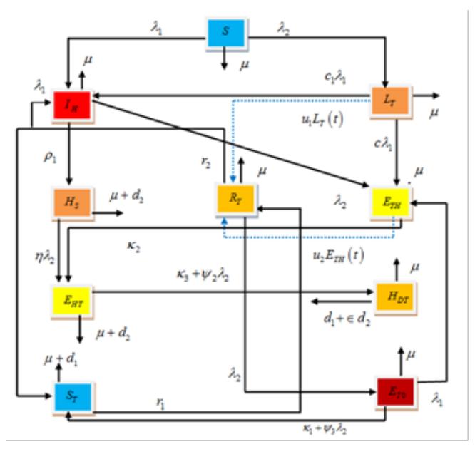
Figure 2.1: Transmission diagram of the HIV-TB interaction with the application of optimal control.
\[\frac{dS(t)}{dt} = A - \lambda_2 S - \lambda_1 S - \mu S, \tag{4}\]
\[\frac{dL_T(t)}{dt} = \lambda_2 S - \lambda_1 L_T (cE_T H + c_1 I_H) - \mu L_T - u_1 L_T, \tag{5}\]
\[\frac{dI_H(t)}{dt} = \lambda_1 S + \lambda_1 R_T - (\rho_1 + \mu) I_H - \lambda_2 I_H + c_1 \lambda_1 L_T I_H, \tag{6}\]
\[\frac{dH_S(t)}{dt} = \rho_1 I_H - \eta \lambda_2 H_S - (\mu + d_2) H_S, \tag{7}\]
\[\frac{dE_{TH}(t)}{dt} = \lambda_1 E_{T0} + \lambda_2 I_H + c\lambda_1 L_T E_{TH} - (\kappa_2 + \mu) E_{TH} - u_2 E_{TH}, \tag{8}\]
\[\frac{dE_{HT}(t)}{dt} = \kappa_2 E_{TH} + \eta \lambda_2 H_S - (\kappa_3 + \mu + d_2 + \psi_2 \lambda_2) E_{HT}, \tag{9}\]
\[\frac{dH_{DT}(t)}{dt} = (\kappa_3 + \psi_2 \lambda_2) E_{HT} - (\mu + d_1 + \epsilon d_2) H_{DT}, \tag{10}\]
\[\frac{dE_{T0}(t)}{dt} = \lambda_2 R_T - (\lambda_1 + \psi_3 \lambda_2) E_{T0} - (\mu + \kappa_1) E_{T0}, \tag{11}\]
\[\frac{dS_T(t)}{dt} = r_2 R_T + (\kappa_1 + \psi_3 \lambda_2) E_{T0} - (\mu + r_1 + d_1) S_T, \tag{12}\]
\[\frac{dR_T(t)}{dt} = r_1 S_T - (\mu + r_2 + \lambda_1 + \lambda_2) R_T + u_1 L_T + u_2 E_{TH}. \tag{13}\]
Considering the initial conditions S(0) = S0 > 0, LT (0) = LT0 ≥ 0, IH(0) = IH0 ≥ 0, HS(0) = HS0 ≥ 0, ETH(0) = ETH0 ≥ 0, EHT (0) = EHT0 ≥ 0, HDT (0) = HDT0 ≥ 0, ET0(0) = ET00 ≥ 0, ST (0) = ST0 ≥ 0, RT (0) = RT0 ≥ 0.
Here the model is now transformed into the optimal control model and (u1(t), u2(t)) are Lebesgue measures belonging to U, where U = (u1(t), u2(t)) : 0 ≤ ai ≤ ui(t) ≤ bi ≤ 1, i = 1, 2, ∀t ∈ [0, T].
Now we take the control variables under consideration and build up the performance index function as following
Minimize \(J(u_1, u_2) = \int_0^T \left( L_T(t) + I_{TH}(t) + \frac{Au_1^2}{2} + \frac{Bu_2^2}{2} \right) dt.\) (14)
The constant A represents the costs associated with vaccine of Latent TB with no HIV and B represents the costs associated with HIV infected individuals (pre-AIDS) co-infected with active TB. So, our model can be stated in the following form [23],
\[\begin{array}{lcl} \text{Minimize } J(x,u) & = & \displaystyle \int_0^T L(x(t),u(t))dt, \\ \text{subject to} & & \\ \dot{x}(t) & = & f(x(t)) + g(x(t))u(t), \forall t \in [0,T], \\ u(t) & \in & U, \ \forall t \in [0,T] \\ x(0) & = & x_0, \end{array} \tag{15}\] where
\[x(t) = \begin{pmatrix} S(t) \\ L_T(t) \\ I_H(t) \\ H_S(t) \\ E_{TH}(t) \\ E_{HT}(t) \\ H_{DT}(t) \\ E_{T0}(t) \\ S_T(t) \\ R_T(t) \end{pmatrix}, \ g(x) = \begin{pmatrix} 0 & 0 \\ -L_T(t) & 0 \\ 0 & 0 \\ 0 & 0 \\ 0 & -E_{TH}(t) \\ 0 & 0 \\ 0 & 0 \\ 0 & 0 \\ 0 & 0 \\ L_T & E_{TH} \end{pmatrix},\]
\[f(x) = \begin{pmatrix} A - \lambda_2 S - \lambda_1 S - \mu S \\ \lambda_2 S - \lambda_1 L_T (c E_{TH} + c_1 I_H) - \mu L_T \\ \lambda_1 S + \lambda_1 R_T - (\rho_1 + \mu) I_H - \lambda_2 I_H + c_1 \lambda_1 L_T I_H \\ \rho_1 I_H - \eta \lambda_2 H_S - \mu H_S - d_2 H_S \\ \lambda_1 E_{T0} + \lambda_2 I_H - c \lambda_1 L_T E_{TH} - (\kappa_2 + \mu) E_{TH} \\ \kappa_2 E_{HT} + \eta \lambda_2 H_S - (\kappa_3 + \mu + d_2 + \psi_2 \lambda_2) E_{HT} \\ (\kappa_3 + \psi_2 \lambda_2) E_{HT} - (\mu + d_1 + \epsilon d_2) H_{DT} \\ \lambda_2 R_T - (\lambda_1 + \psi_3 \lambda_2) E_{T0} - (\mu + \kappa_1) E_{T0} \\ r_2 R_T + (\kappa_1 + \psi_3 \lambda_2) E_{T0} - (\mu + r_1 + d_1) S_T \\ r_1 S_T - (\mu + r_2 + \lambda_1 + \lambda_2) R_T (t) + u_1 L_T + u_2 E_{TH} \end{pmatrix}.\]
\(u(t) = \begin{pmatrix} u_1(t) \\ u_2(t) \end{pmatrix}\) and we set the integrand of the performance index as
\[L(x,u) = L_T(t) + I_{TH}(t) + \frac{1}{2}(Au_1^2 + Bu_2^2).\] (16)
3. EXISTENCE OF THE STATE VARIABLES
We recall the state equations (4)-(13) with initial conditions. If all the equations of the system (4)-(13) are added together, we obtain the equation as follows:
\[\frac{dN(t)}{dt} = \frac{dS(t)}{dt} + \frac{dL_T(t)}{dt} + \frac{dI_H(t)}{dt} + \frac{dH_S(t)}{dt} + \frac{dE_{TH}(t)}{dt} + \frac{dE_{HT}(t)}{dt} + \frac{dH_{DT}(t)}{dt} + \frac{dE_{T0}(t)}{dt} + \frac{dS_T(t)}{dt} + \frac{dR_T(t)}{dt},\] \[\frac{dN(t)}{dt} = A - \mu N - d_2(H_S + E_{TH} + \in H_{DT}) - d_1(S_T + H_{DT}),\]
\[\therefore \frac{dN(t)}{dt} \le A - N(t) \implies N(t) \le \frac{A}{\mu} + (N_0 - \frac{A}{\mu}e^{-\mu t}) = V_1 \in \mathbb{R}_+,\] and \(\lim_{t\to\infty}\sup N(t)\leq V_1\). it means \(S(t),L_T(t),I_H(t),H_S(t),E_{TH}(t),E_{HT}(t),H_{DT}(t),E_{T0}(t),S_T(t),R_T(t)\leq V_1\) as \(t\to\infty\). Now, if \(\theta_t\) indicates the derivative of \(\theta\) with respect to time t, the system (4)-(13) may be written as
\[\theta_t = P\theta + F(\theta),\tag{17}\] where,
\[\text{[rumus tidak dapat ditampilkan dengan baik — lihat PDF asli]}\]
Equation (17) being a non-linear system, it has a bounded coefficient. Now we set \(D(\theta) = \theta_t = P\theta + F(\theta)\). We need the boundedness of the system for finite time to obtain the optimal control. Consider for \(u \in U\), then there exists a bounded solution such that \(|F(\theta_1) - F(\theta_2)| \leq M|\theta_1 - \theta_2|\), where \(M = 2gV_1\). Again set \(|D(\theta_1) - D(\theta_2)| \leq ||P|||\theta_1 - \theta_2| + M|\theta_1 - \theta_2| \leq V|\theta_1 - \theta_2|\) where \(V = Max(M, ||P||) < \infty\).
Therefore, we can say the function D is uniformly Lipschitz continuous. As a result of the notion of control, we may deduce that the system (17) must have a solution.
4. EXISTENCE OF THE OBJECTIVE FUNCTIONAL
Consider the optimal control problem below:
\[J(u_1, u_2) = \int_0^T (L_T(t) + I_{TH}(t) + (Au_1^2/2) + (Bu_2^2/2))dt,\] (18)
where T is the treatment period i.e., the time when the TB infected individuals are taken under treatment. We now seek to reduce the number of affected people in this time frame. We use the following theorems to prove the existence of the objective functional.
Theorem 4.1. We consider an n-variable system.
\[\bar{x} = \begin{pmatrix} x_1(t) \\ \vdots \\ x_n(t) \end{pmatrix}.\]
Assume u(t) is a control variable with a set of permissible controls U that satisfies the differential equation \(x_i'(t) = g(t, x_i(t), u(t))\) for i = 1, ..., n with associated objective functional \(J(u) = \int f(t, \bar{x}(t), u(t)) dt\). Then, if the following requirements are met, there is a best-practice control that reduces \(\bar{J}(u)\). \ni) F is not an empty set. ii) U must be a closed and convex control set. iii) The right-hand side of the state system is continuous, bounded above by a linear combination of control and state, and may be expressed as a linear function of u with time and state as coefficients and iv) The objective functional's integrand is convex on U and is bounded below by A. \(-C_2 + C_1(u)^{\eta}\), with \(C_1 > 0\) and \(\eta > 0\) [1].
Proof (i): Let
\begin{array}{rclcrcl} S' & = & F_1(t,S,L_T,I_H,H_S,E_{TH},E_{HT},H_{DT},E_{T0},S_T,R_T), \\ L'_T & = & F_2(t,S,L_T,I_H,H_S,E_{TH},E_{HT},H_{DT},E_{T0},S_T,R_T), \\ I'_H & = & F_3(t,S,L_T,I_H,H_S,E_{TH},E_{HT},H_{DT},E_{T0},S_T,R_T), \\ H'_S & = & F_4(t,S,L_T,I_H,H_S,E_{TH},E_{HT},H_{DT},E_{T0},S_T,R_T), \\ E'_{TH} & = & F_5(t,S,L_T,I_H,H_S,E_{TH},E_{HT},H_{DT},E_{T0},S_T,R_T), \\ E'_{HT} & = & F_6(t,S,L_T,I_H,H_S,E_{TH},E_{HT},H_{DT},E_{T0},S_T,R_T), \\ H'_{DT} & = & F_7(t,S,L_T,I_H,H_S,E_{TH},E_{HT},H_{DT},E_{T0},S_T,R_T), \\ E'_{T0} & = & F_8(t,S,L_T,I_H,H_S,E_{TH},E_{HT},H_{DT},E_{T0},S_T,R_T), \\ S'_T & = & F_9(t,S,L_T,I_H,H_S,E_{TH},E_{HT},H_{DT},E_{T0},S_T,R_T), \\ R'_T & = & F_{10}(t,S,L_T,I_H,H_S,E_{TH},E_{HT},H_{DT},E_{T0},S_T,R_T) \end{array}
where \(F_1, F_2, F_3, F_4, F_5, F_6, F_7, F_8, F_9\), and \(F_{10}\) met up the right side of the system of equations (4)-(13). If C is any constant then, let u(t) = C. So, \(F_1, F_2, F_3, F_4, F_5, F_6, F_7, F_8, F_9\), and \(F_{10}\) with respect to state variables and constants are also continuous everywhere. As a result, there is a unique solution \(S = \sigma_1(t), L_T = \sigma_2(t), I_H = \sigma_3(t), H_S = \sigma_4(t), E_{TH} = \sigma_5(t), E_{HT} = \sigma_6(t), H_{DT} = \sigma_7(t), E_{T0} = \sigma_8(t), S_T = \sigma_9(t), R_T = \sigma_10(t)\) satisfying the initial conditions. From above, we can say the set of control variables and the corresponding state variables are non-empty. Hence the stated condition (i) is accomplished.
Proof (ii): U is closed by the definition and we now take two control variables \((u_1, u_2)\) belong to U. Again we consider \(\theta\) between 0 and 1 such that \(0 \le \theta u_1 + (1 - \theta)u_2\). We also find that \(\theta u_1 \le \theta\) and \((1 - \theta)u_2 \le (1 - \theta)\).
Then \(\theta u_1 + (1 - \theta)u_2 \le \theta + (1 - \theta) = 1\).
Hence, \(0 \le \theta u_1 + (1 - \theta)u_2 \le 1\) for all \(u_1, u_2 \in U\) and \(\theta \in [0, 1]\). So, U is convex and the condition (ii) is satisfied.
Proof (iii): We consider
F_1 \leq A - \mu S, F_2 \leq -\mu L_T - u_1 L_T, F_3 \leq -(\rho_1 + \mu) I_H, F_4 \leq \rho_1 I_H - (\mu + d_2) H_S, F_5 \leq -(\kappa_2 + \mu) E_{TH} - u_2 E_{TH}, F_6 \leq \kappa_2 E_{HT} - (\kappa_3 + \mu + d_2) E_{HT}, F_7 \leq \kappa_3 E_{HT} - (\mu + d_1 + \epsilon d_2) H_{DT}, F_8 \leq -(\mu + \kappa_1) E_{T0}, F_9 \leq r_2 R_T + \kappa_1 E_{T0} - (\mu + r_1 + d_1) S_T, F_{10} \leq r_1 S_T - (\mu + r_2) R_T + u_1 L_T + u_2 E_{TH}.
Then the system (18) can be written as
\[\text{[rumus tidak dapat ditampilkan dengan baik — lihat PDF asli]}\] where
\[\bar{n} \left( t, \begin{vmatrix} S \\ L_T \\ I_H \\ H_S \\ E_{TH} \\ E_{HT} \\ H_{DT} \\ E_{T0} \\ S_T \\ R_T \end{vmatrix} \right) = \begin{pmatrix} 0 & 0 \\ -L_T & 0 \\ 0 & 0 \\ 0 & 0 \\ 0 & -E_{TH} \\ 0 & 0 \\ 0 & 0 \\ 0 & 0 \\ 0 & 0 \\ L_T & E_T H \end{pmatrix},\]
\[\text{[rumus tidak dapat ditampilkan dengan baik — lihat PDF asli]}\]
This results in a linear control function u, which is determined by time and state variables. We must determine the right-hand side's boundary. Assume that all of the parameters are constant and equal to or larger than zero. Now we can write \(|\bar{F}(t,\bar{X},u)| \leq ||\bar{m}|||\bar{X}| + |\bar{L}_T||\bar{E}_{TH}||u(t)| \leq p(|\bar{X}| + |u(t)|)\). Here \(\bar{L}_{TH}\) and \(\bar{E}_{TH}\) are bounded and p contains the upper bound of the constant matrix. As a result, the right-hand side is bounded by the sum of the state and the control. So, the condition stated by (iii) is proved.
Proof (iv): The integrand of the objective functional is taken into consideration as \(f(u) = L_T(t) + E_{TH}(t) + u^2\) where \(Au_1^2/2 + Bu_2^2/2 = u^2\) and the two control variables \((u_1, u_2)\) belong to U and \(0 < \omega < 1\). Then this can be written as written as \[(u_1 - u_2)^2 = u_1^2 - 2u_1u_2 + u_2^2 \ge 0,\] \[\Rightarrow u_1^2 + u_2^2 \ge 2u_1u_2,\] \[\Rightarrow \omega(1 - \omega)u_1^2 + \omega(1 - \omega)u_2^2 \ge \omega(1 - \omega)u_1u_2 \ge (\omega u_1 + (1 - \omega)u_2)^2,\] \[\Rightarrow (L_T(t) + E_{TH}(t)) + \omega u_1^2 + (1 - \omega)u_2^2 \ge (L_T(t) + E_{TH}(t)) + (\omega u_1 + (1 - \omega)u_2)^2,\] \[\Rightarrow (L_T(t) + E_{TH}(t)) + (\omega + (1 - \omega)) + (\omega u_1^2 + (1 - \omega)u_2^2 \ge (L_T(t) + E_{TH}(t)) + (\omega u_1 + (1 - \omega)u_2)^2,\] \[\Rightarrow \omega f(u_1) + (1 - \omega)f(u_2) \ge f(\omega u_1 + (1 - \omega)u_2),\] which implies that f(u) is convex on U. Now we have to show that \(J(u) \geq -C_2 + C_1(u)^\eta\) with \(\eta > 0, C_1 \geq 0\). Now \(J(u) = L_T(t) + E_{TH}(t) + Au_1^2/2 + Bu_2^2/2\) and since \(Au_1^2/2 + Bu_2^2/2 = u^2\) then \(J(u) = L_T(t) + Bu_1^2/2 + Bu_2^2/2 = u^2\)
\(E_{TH}(t)+u^2\). \(\therefore J(u) \geq -[L_T(t)+E_{TH}(t)]+u^2=-C_2+C_1u^2\), where \(C_2>0\) that depends on the upper bound of \(L_T(t)\) and \(E_{TH}(t)\). We also find that \(\eta=2>1,C_1>0\). So, condition stated by (iv) is completed and the existence of objective functional is established.
5. CHARACTERIZATION OF OPTIMAL CONTROL
We must construct necessary conditions for optimal control in order to characterize it, and in this case, Pontryagin Maximum principle is utilized to the Hamiltonian H. With respect to \((u_1,u_2)\) we can state the standard Hamiltonian function as \(H(t,x(t),u(t),p(t),\lambda(t))=\langle p(t),f(x(t))+g(x(t)u(t))\rangle-\lambda L(x(t),u(t))\) \(\lambda\in\mathbb{R}\), where the adjoint variables are denoted as \(p=(p_S+p_{L_T},p_{I_H},p_{H_S},p_{E_{TH}},p_{E_{HT}},p_{H_{DT}},p_{E_{T0}},p_{S_T},p_{R_T})\in\mathbb{R}^{10}\). Let the pair \((x^*,u^*)\) be the best solution to the optimal control issue described above. Then the maximum principal claims the existence of a scalar \(\lambda_0\geq 0\), an absolute continuous function p(t) such that the following conditions are satisfied:
i) \max \{|p(t)|: t \in [0,T]\} + \lambda_0 > 0,
\nii) p(t) = \lambda L_x[t] - \langle p[t], f_x[t] + g_x[t]u^*(t) \rangle,
\niii) p(t) = (0,0),
\niv) H = (x^*(t), u^*(t), p(t)) = \max_{x} H(x^*(t), p(t), u(t)), where a_1 \le u_1 \le b_1, a_2 \le u_2 \le b_2.
From equation (ii) with \(\lambda = 1\) i.e., adjoint equations in normal form are explicitly given by
\begin{split} p_S' &= -(\partial H/\partial S) = \lambda_1 (p_S - P_{I_H}) + \lambda_2 (p_S - p_{L_T}) + P_S \mu, \\ P_{L_T}' &= -(\partial H/\partial L_T) = \lambda_1 \{ P_{L_T} (c E_{TH} + c_1 I_H) - P_{I_H} c_1 I_H + P_{E_{TH}} c_2 E_{TH} \} + P_{L_T} (\mu - u_1) - P_{E_{T0}} - P_{R_T} u_1, \\ P_{I_H}' &= -(\partial H/\partial I_H) = \lambda_1 (P_{L_T} L_T c_1 - P_{I_H} c_1 L_T) + \lambda_2 (P_{I_H} - P_{E_{TH}} \lambda_2) + P_{I_H} (\rho_1 + \mu) - P_{H_S} \rho_1, \\ P_{H_S}' &= -(\partial H/\partial H_S) = P_{H_S} (\mu + d_2) + \lambda_2 \eta (P_{H_S} - P_{E_{TH}}, \\ P_{E_{TH}}' &= -(\partial H/\partial E_{TH}) = P_{E_{TH}} (c \lambda_1 L_T + \kappa_2 + \mu + u_2) + P_{L_T} \lambda_1 L_T c - P_{R_T} u_2, \\ P_{E_{HT}}' &= -(\partial H/\partial E_{HT}) = P_{E_{HT}} (-\kappa_2 + \kappa_2 + \mu + d_2 + \psi_2 \lambda_2) - P_{H_{DT}} (\kappa_3 + \psi_2 \lambda_2), \\ P_{H_{DT}}' &= -(\partial H/\partial H_{DT}) = P_{H_{DT}} (\mu + d_1 + \in d_2), \\ P_{E_{T0}} &= -(\partial H/\partial E_{T0}) = P_{E_{T0}} (\lambda_1 + \psi_3 \lambda_2 + \mu + \kappa_1) - P_{S_T} (\kappa_1 + \psi_3 \lambda_2), \\ P_{S_T}' &= -(\partial H/\partial R_T) = P_{S_T} (\mu + r_1 + d_1) - P_{R_T} r_1, \\ P_{R_T}' &= -(\partial H/\partial R_T) = P_{R_T} (\mu + r_2 + \lambda_1 + \lambda_2) - P_{S_T} r_2 - P_{E_{T0}} \lambda_2 - P_{I_H} \lambda_1. \end{split}
with the transversality condition \(p_i(T) = 0, i = 1, 2, 3, ..., 10\). We can now demonstrate the existence of optimum control by using the Pontryagin Maximum Principle.
Theorem 5.1. There exists optimal control \((u_1^*, u_2^*)\) that minimizes the objective functional J over U given by \(u_1^* = \max\{0, \min(1, (P_{L_T} - P_{R_T})L_T^*/A)\}\) and \(u_2^* = \max\{0, \min(1, (P_{E_{TH}} - P_{R_T})E_{TH}/B)\}\).
Proof: We search for the characterization of \(u_1^*\) and \(u_2^*\), where three cases arise for
\begin{aligned} u_1^* &= \max\{0, \min(1, (P_{L_T} - P_{R_T}) L_T^* / A)\} \text{ and } u_2^* &= \max\{0, \min(1, (P_{E_{TH}} - P_{R_T}) E_{TH} / B)\}. \\ \text{Now } \partial H / \partial u_1 &= A u_1 - P_{L_T} L_T + P_{R_T} L_T \\ \textbf{Case I: When } \partial H / \partial u_1 &> 0, \text{ then } A u_1 - P_{L_T} L_T > 0 \implies A u_1 > P_{L_T} L_T - P_{R_T} L_T \implies A u_1 > (P_{L_T} - P_{R_T}) L_T / A. \text{ Let } (P_{L_T} - P_{R_T}) L_T / A = \bar{u}_1. \text{ So } u_1 > \bar{u}_1 : 0 \geq \bar{u}_1. \\ \textbf{Case II: When } \partial H / \partial u_1 &= 0, \text{ then } A u_1 - P_{L_T} L_T = 0 \implies A u_1 = P_{L_T} L_T - P_{R_T} L_T \implies A u_1 = (P_{L_T} - P_{R_T}) L_T / A \implies 0 < (P_{L_T} - P_{R_T}) L_T / A < 1 : 0 < \bar{u}_1 < 1. \\ \textbf{Case III: When } \partial H / \partial u_1 &= 0, \text{ then } A u_1 - P_{L_T} L_T < 0 \implies A u_1 < P_{L_T} L_T - P_{R_T} L_T \implies A u_1 < (P_{L_T} - P_{R_T}) L_T / A : 1 \leq \bar{u}_1. \text{ Therefore } u_1^* = \{0 \text{ if } \bar{u}_1 \leq 0, \bar{u}_1 \text{ if } 0 < \bar{u}_1 < 1, 1 \text{ if } \bar{u}_1 \geq 1. \text{ In short form} \end{aligned}
Again, for the characterization of \(u_2^*\), we get \(\partial H/\partial u_2 = Bu_2 - P_{E_{TH}}E_{TH} + P_{R_T}E_{TH}\). Case I: When \(\partial H/\partial u_2 > 0\), then \(Bu_2 - P_{E_{TH}}E_{TH} + P_{R_T}E_{TH} > 0 \implies Bu_2 > P_{E_{TH}}E_{TH} - P_{R_T}E_{TH} \implies Bu_2 > (P_{E_{TH}} - P_{R_T})E_{TH} \implies u_2 > (P_{E_{TH}} - P_{R_T})E_{TH}/B\). Let \((P_{E_{TH}} - P_{R_T})E_{TH}/B = \bar{u}_2 \implies u_2 > \bar{u}_2 \implies 0 > \bar{u}_2\).
\(\text{[rumus tidak dapat ditampilkan dengan baik — lihat PDF asli]}\)
\[u_2^* = \max\{0, \min(1, (P_{E_{TH}} - P_{R_T})E_{TH}/B)\}. \tag{20}\]
Now from (19) and (20), we get
\[\begin{cases} 0 & \text{if } & \bar{u}_i \le 0, \\ \bar{u}_i & \text{if } & 0 < \bar{u}_i < 0, \\ 1 & \text{if } & \bar{u}_i \ge 1. \end{cases}\] (21)
This completes the proof.
5.1. Basic Reproduction Ratio
The basic reproduction ratio, denoted by \(R_0\), can be derived using the next generation matrix. Here in \(u_2\) does not have any effect on \(R_0\) since \(E_{TH}\) and \(H_{DT}\) does not contribute in the next generation matrix (NGM). The resulting basic reproduction number is given by:
R_0 = \max(R_{01}, R_{02}) with:
R_{01} = \frac{(\eta_2\rho_1 + \mu + d_2)\beta_1}{(\rho_1 + \mu)(\mu + d_2)}, R_{02} = \frac{(\mu^2 + \mu d_1 + \mu \kappa_1 + \mu r_1 + d_1 \kappa_1 + \kappa_1 r_1)\beta_2 c}{(\mu + u_1)(\mu + \kappa_1)(\mu + r_1 + d_1)}. R_{01} \text{ is independent of the control } u_1. \text{ Let us concentrate on the effect of } u_1 \text{ on } R_{02}. \text{ In this case we obtain ratio}
\[\frac{R_{02}(u_1 \neq 0)}{R_{02}(u_1 = 0)} = \frac{\mu}{\mu + u_1} < 1,\] which indicates that the control indeed is able to reduce the basic reproduction number. Hence if we would like to reduce the basic reproduction number down to p% of the original basic reproduction number then it can be deduced that the minimum control effort needed is \(u_1 \geq (1-p)(\mu)\).
6. NUMERICAL SIMULATIONS AND DISCUSSION
In this section we discuss the numerical simulations with the responsible parameters \(\beta_1\) and \(\beta_2\). Our view indicates that these two metrics, the HIV disease contact rate and the TB disease contact rate, are mostly responsible for the severe threat. So, we intend to control these parameters by applying two controls measures, the vaccination control and the treatment control. To illustrate this, we have considered three cases. Firstly, we have considered the vaccination \((u_1 \neq 0, u_2 = 0)\). Secondly, we have considered the treatment control \((u_1=0,u_2\neq 0)\) and finally we have considered both the treatment control and the vaccination control \((u_1 \neq 0, u_2 \neq 0).\)
Case I: In this case we will apply only the vaccination control \((u_1)\) to the numerical simulations and the treatment control \((u_2)\) is absent, that means control \((u_1 \neq 0, u_2 = 0)\). The simulation results are represented in Figures 6.2-6.11.
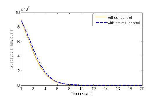
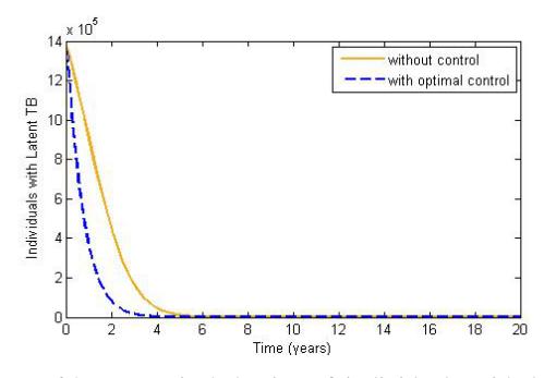
Figures 6.2-6.11 show the dynamics of ten compartments for cost functional (18), \(\beta_1 = 0.2, \beta_2 = 0.1\) and parameters value from Table 6.1 in case of vaccination \((u_1)\) as optimal control. Observe that the number of HIV and TB disease individuals S and laten TB individuals \(L_T\) decrease significantly when only the vaccination control measure \(u_1\) is implemented in Figures 6.2 and 6.3. As opposed to the people stay in class \(I_H\) and \(H_S\) increase to the number of individuals that have TB or and AIDS, see Figures 6.4 and 6.5 with out treatment control measure. In both classes the individuals increase more rapidly when control is executed than without control. In the 20 years of total infectious period persons in the groups HIV infected individuals (pre-AIDS) exposed to TB, AIDS individuals exposed to TB, AIDS individuals dually infected with TB, Symptoms of TB, and Exposed to TB only diminish when the vaccine control is employed, see in the Figures 6.6-6.10. After twelve years \(E_{T0}\) class goes stable showing the sharp decreasing feature compared to the vaccination. Recovered individuals response to a great extent in vaccination control, as see in Figure 6.11 that in the thirteen year the population cured out and the class goes to asymptotically stable.
| - | ||
|---|---|---|
| Parameters | Descriptions of the parameters | Values of the parameters |
| \(\overline{A}\) | Recruitment rate of Susceptible Individuals | \(0.029 \ (yr^{-1})\) |
| c | Number of Contacts having only HIV and no TB | \(2.0 \ (yr^{-1})\) |
| \(c_1\) | Number of Contacts having HIV and TB | \(0.50 (yr^{-1})\) |
| \(d_1\) | Death Rate Related to TB | \(0.1 \ (yr^{-1})\) |
| \(d_2\) | Death Rate Related to AIDS | \(0.333(yr^{-1})\) |
| \(\beta_1\) | Contact or Disease Transmission Rate of HIV | \(0.20 - 0.70 (yr^{-1})\) |
| \(\beta_2\) | Contact or Disease Transmission Rate of TB | \(0.10 - 0.90 \ (yr^{-1})\) |
| \(r_1\) | Natural Recovery Rate | \(0.2 \ (yr^{-1})\) |
| \(r_2\) | Relapsing Rate for the Individuals with Symptom of TB | \(0.00001 (yr^{-1})\) |
| \(\psi_1,\psi_2,\psi_3,\in\) | Modification Parameter | \(1.07, 1.101, 0.71, 1.2 (yr^{-1})\) |
| \(\eta, \eta_1, \eta_2, \eta_3, \in\) | Modification Parameter | 1.2,1.05,1.02,1.10 (Dimensionless) |
| \(\kappa_1\) | TB Propagation Rate | \(0.000113 \ (yr^{-1})\) |
| \(\kappa_2\) | HIV Infected Rate with Mtb Progress to AIDS | \(0.102 \ (yr^{-1})\) |
| \(\kappa_3\) | AIDS Cases Infected Rate with Mtb Progress | \(0.0002 (yr^{-1})\) |
| \(\mu\) | Natural Mortality Rate | \(0.01 \ (yr^{-1})\) |
Table 6.1: The values of parameters and their descriptions [11]
\(\rho_1\)
Rate of progression to AIDS
Figure 6.2: Dynamic behavior of susceptible individuals considering vaccination \((u_1)\) as optimal control.
\(0.1 \ (yr^{-1})\)
Figure 6.3: Dynamic behavior of individuals with latent TB considering vaccination \((u_1)\) as optimal control.
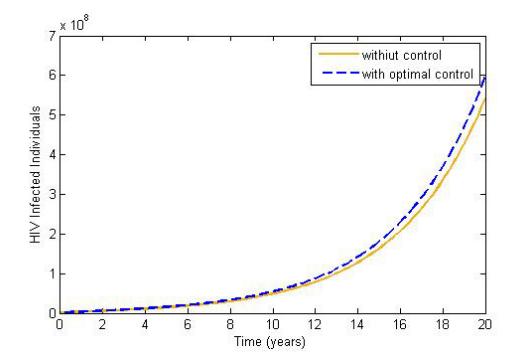
Figure 6.4: Dynamic behavior of HIV infected individuals considering vaccination \((u_1)\) as optimal control.
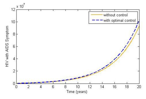
Figure 6.5: Dynamic behavior of HIV with AIDS symptom considering vaccination \((u_1)\) as optimal control.
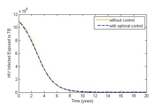
Figure 6.6: Dynamic behavior of HIV infected exposed to TB considering vaccination (u1) as optimal control.
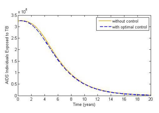
Figure 6.7: Dynamic behavior of AIDS individuals exposed to TB considering vaccination (u1) as optimal control.
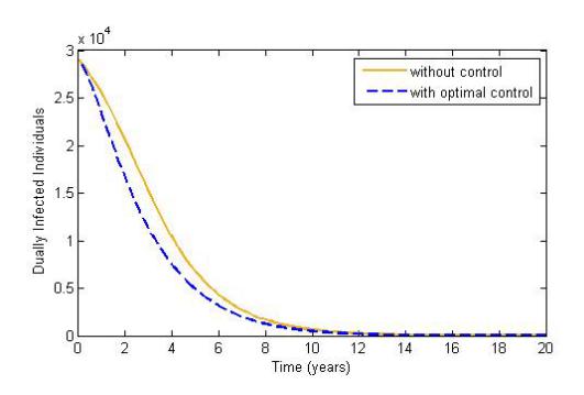
Figure 6.8: Dynamic behavior of AIDS individuals dually infected with TB considering vaccination (u1) as optimal control.
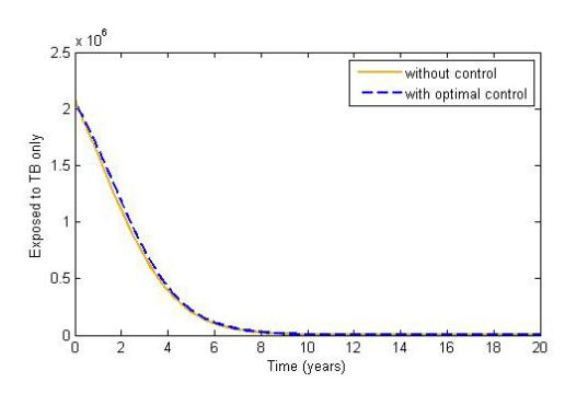
Figure 6.9: Dynamic behavior of exposed to TB individuals considering vaccination (u1) as optimal control.
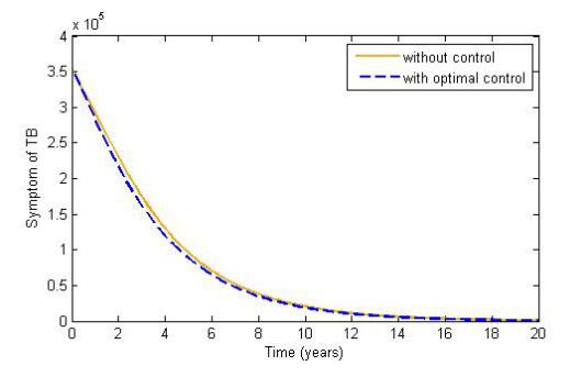
Figure 6.10: Dynamic behavior of symptom of TB considering vaccination (u1) as optimal control.
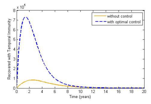
Figure 6.11: Dynamic behavior of recovered with temporal considering vaccination (u1) as optimal control.
Case II: In this case we will apply only the treatment control (u2) to the numerical simulations and the vaccination control (u1) is absent, that means control (u1 = 0, u2 ̸= 0). Then the simulation results are represented in Figures 6.2-6.11.
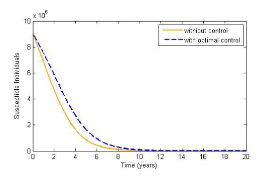
Figure 6.12: Dynamic behavior of susceptible Individuals considering treatment (u2) as optimal control.
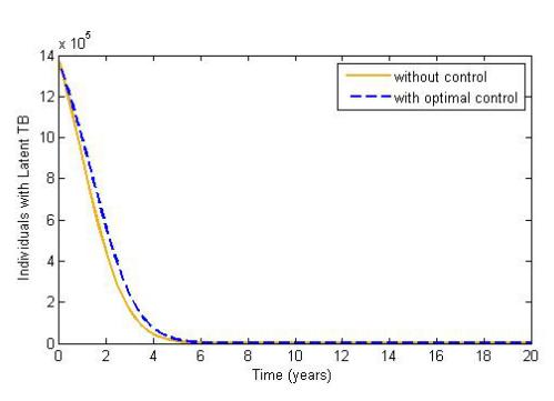
Figure 6.13: Dynamic behavior of individuals with latent TB considering treatment (u2) as optimal control.
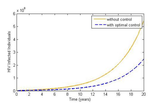
Figure 6.14: Dynamic behavior of HIV infected individuals considering treatment (u2) as optimal control.
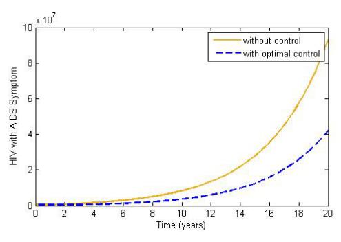
Figure 6.15: Dynamic behavior of HIV with AIDS symptom considering treatment (u2) as optimal control.
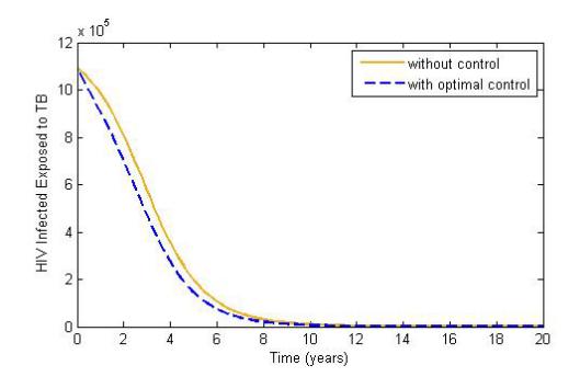
Figure 6.16: Dynamic behavior of HIV infected exposed to TB considering treatment (u2) as optimal control.
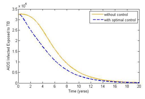
Figure 6.17: Dynamic behavior of AIDS individuals exposed to TB considering treatment (u2) as optimal control.
Figures 6.12-6.21 show the dynamics of ten compartments for cost functional (18), β1 = 0.2, β2 = 0.1 and parameters value from Table 6.1 in case of treatment (u2) as optimal control. Observe that the number of HIV and TB disease individuals S and laten TB individuals LT decrease considerably when the treatment control
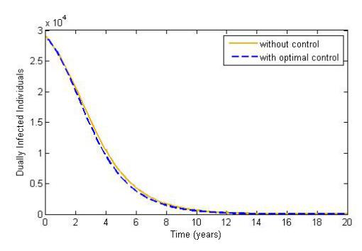
Figure 6.18: Dynamic behavior of AIDS individuals dually infected with TB considering treatment (u2) as optimal control.
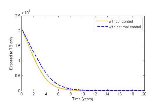
Figure 6.19: Dynamic behavior of exposed to TB individuals considering treatment (u2) as optimal control.
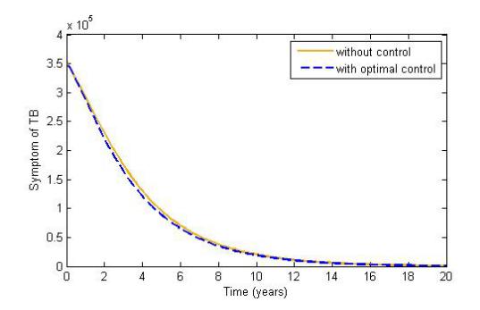
Figure 6.20: Dynamic behavior of symptom of TB considering treatment (u2) as optimal control.
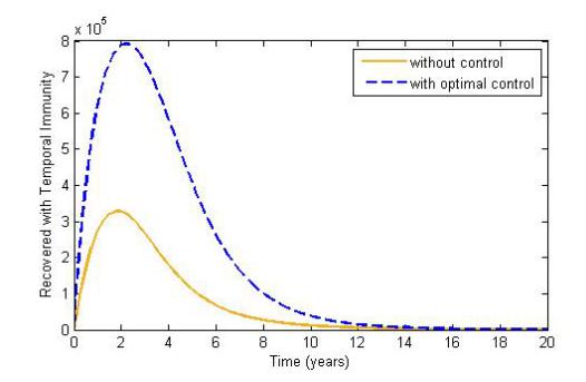
Figure 6.21: Dynamic behavior of recovered with temporal considering treatment (u2) as optimal control.
measure u2 is applied, but vaccination control is more effective than treatment for both of the classes, as seen in Figures 6.12 and 6.13. On the alternative the number of people that stay in class IH and HS increase considerably, see Figures 6.14 and 6.15 with treatment control measure. In both classes the individuals increase less rapidly when control is executed than without control. During the execution period the individuals in the classes HIV infected individuals (pre-AIDS) exposed to TB ETH, AIDS individuals exposed to TB EHT , AIDS individuals dually infected with TB HDT , Symptom of TB ST and Exposed to TB only ET0 decrease when the treatment control is used with the exclusion of class ET0, see in the Figures 6.16-6.20. Class ET0 goes stable showing the sharp decreasing feature compared to the treatment after eight years. So, both the controls are separately effective to reduce the HIV/AIDS and TB Co- infection for most of the classes of this system. Temporal recovery individuals' response highly in treatment control, as seen in Figure 6.21 that in the near twelve years the population cured out and the class goes to the stable equilibrium state asymptotically.
Case III: In this case we will apply both the treatment control (u2) and the vaccination control (u1) to the numerical simulations that means control (u1 ̸= 0, u2 ̸= 0). The computational results are shown in Figures 6.22-6.31.
Figures 6.22-6.31 shows the variation of ten compartments for cost functional (18), for 20 years of time for different values of β1, β2 and parameters value from Table 6.1 in case of both vaccination control (u1) and treatment control (u2) measures. We examine that the effect of control measures on the class of susceptible individuals S and laten TB individuals LT decrease in the presence of vaccination and treatnemt controls, as seen in Figures 6.22 and 6.23. It is noticed that for susceptible and latent TB classes simultaneous control strategy acceletares the decreasing rate more than single control strategy. Again the control measures lightly influence the number of individuals that stay in class IH and HS increasing to the number of individuals, as seen in Figures 6.24 and 6.25. In both classes the individuals increase lesser when control is imposed
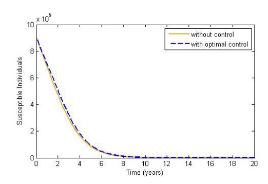
Figure 6.22: Dynamic behavior of Individuals with susceptible considering the control (u1) and control (u2) as optimal control.
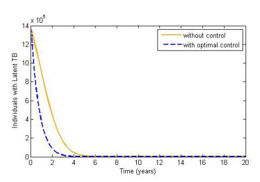
Figure 6.23: Dynamic behavior of individuals with latent TB considering the both optimal control, vaccination control (u1) and treatment control (u2).
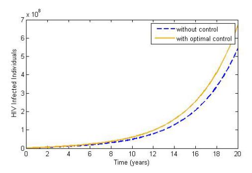
Figure 6.24: Dynamic behavior of HIV infected individuals considering the both optimal control, vaccination control (u1) and treatment control (u2).
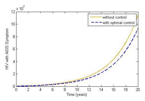
Figure 6.25: Dynamic behavior of HIV with AIDS symptom considering the both optimal control, vaccination control (u1) and treatment control (u2).
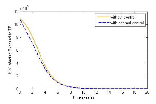
Figure 6.26: Dynamic behavior of HIV infected exposed to TB considering the both optimal control, vaccination control (u1) and treatment control (u2).
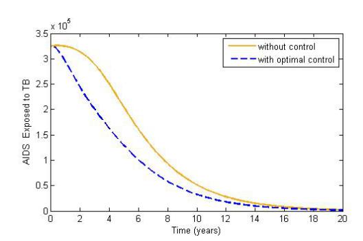
Figure 6.27: Dynamic behavior of AIDS exposed to TB considering the both optimal control, vaccination control (u1) and treatment control (u2).
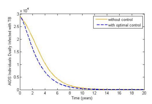
Figure 6.28: Dynamic behavior of AIDS individuals dually infected with TB considering the both optimal control, vaccination control (u1) and treatment control (u2).
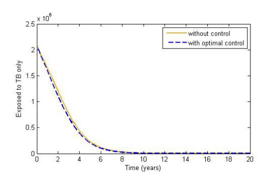
Figure 6.29: Dynamic behavior of exposed to TB only considering the both optimal control, vaccination control (u1) and treatment control (u2).
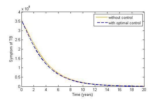
Figure 6.30: Dynamic behavior of symptom of TB considering the both optimal control, vaccination control (u1) and treatment control (u2).
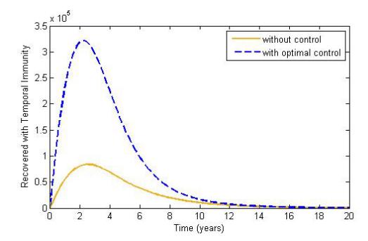
Figure 6.31: Dynamic behavior of recovered with temporal immunity considering the both optimal control, vaccination control (u1) and treatment control (u2).
than without control. During the execution timeline the individuals in the classes HIV infected individuals (pre-AIDS) exposed to TB ETH, AIDS individuals exposed to TB EHT , AIDS individuals dually infected with TB HDT , Symptomatic TB ST and Exposed to TB only ET0 decrease when both the vaccination control measure and treatment control measure are used, as seen in the Figures 6.26-6.30. Temporal recovery individuals increase highly in extreme level with the both control measures, as seen in Figure 6.31. For all these classes the mutual implementation of vaccination and treatment control measures are more effective and is of significant influence on the model. So, both the controls are effective side by side to reduce the HIV/AIDS associated with TB co-infection of this system.
6.1. Effect of Control on Basic Reproduction Ratio
We now present the simulated trajectories of optimal control and the effect of vaccination control on the basic reproduction ratio is shown in Figure 6.32.
From the Figure 6.32(A), we have found that the vaccination control varies to ranges 0 to 0.004. At the initial time the control takes its minimum value and after 7.5 years later it reaches its maximum values that is continued to the fixed final time. This situation gives vaccination control is very effective. Figure 6.32(B) represents, at the initial time the treatment control is maximum. After that, it is starting to decrease and reach its minimum value. Then, after 4 years later it again starts increasing and reaches a steady state position. That means in this model, the effects of control measures are more effective. Figure 6.32(C) represents the effects of control u1 on the basic reproduction number. From the first subplot of Figure 6.32(A), we see that control is the function of time, and from the third subplot of Figure 6.32(C), we see that R0 is the function
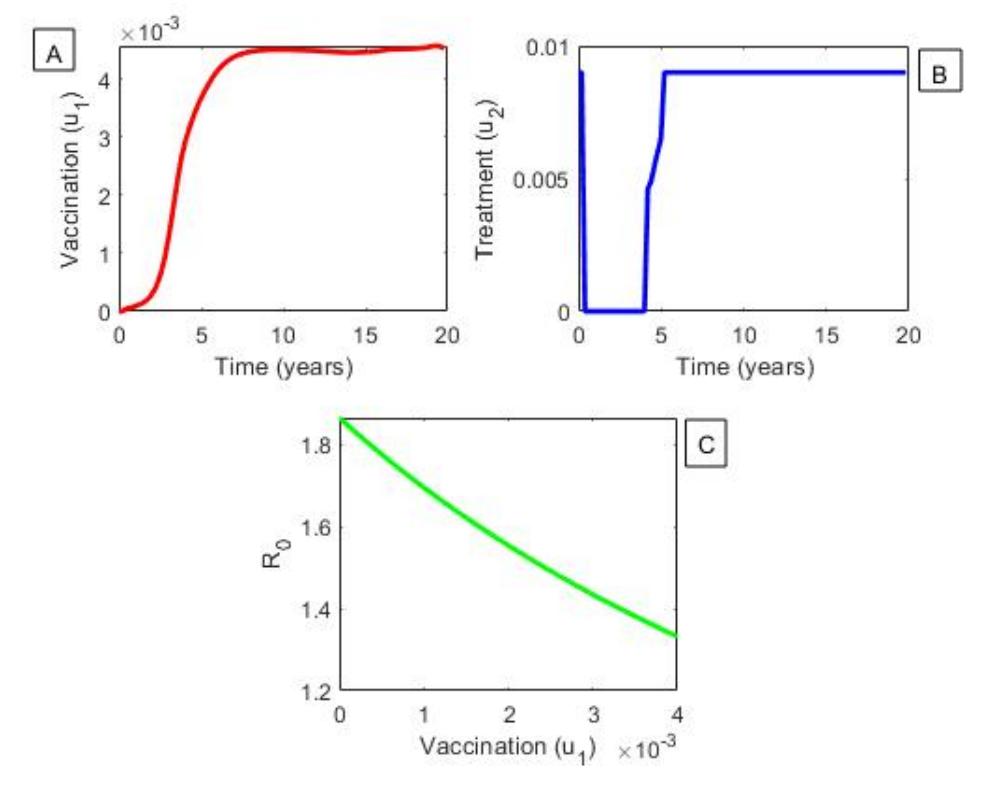
Figure 6.32: represents (A) vaccination control and (B) treatment control behavior with time from 0 to 20 years, (C) shows the effects of vaccination control on basic reproduction number.
of u1. So, we can conclude that R0 is the function of time which is changed both for the parameters and control with times.
From Figure 6.33, we see that basic reproduction number is increasing with the increasing values of per capita contact rate and decreasing with the increasing efforts of vaccination control. So, if we take vaccination control measure and thus reduce the personal contact, then this situation may be manageable.
7. CONCLUSIONS AND FUTURE WORKS
The goal of this work is to investigate the transmission dynamics of HIV/AIDS, tuberculosis, and their co-infections, as well as the use of optimal control in the human body. We employed the possible control measure to reduce the number of HIV, TB and the co-infected individuals from the community. Numerical simulations are carried out to show the interaction, to assess the impact of the different stages during the whole infection period and to find some epidemiological features of this study. The notable findings of this work are to reduce and control the prevalence of HIV and TB infections among the potential and highly infected population. If the individuals have lower infection rate the better scenarios are in a community for HIV /AIDS, TB and HIV-TB co-infection. Without applying the controls (treatment and vaccination) all the infected stages or compartments are upward and the recovered individuals is downward that means the disease is progressive. From the figure of recovered individuals we notice that the individuals are increasing in case of the application of optimal control than without using control. All the compartments except the recovered individuals decrease when we use the optimal control strategy. Numerical analysis represents the individuals with no control and with optimal control that straight forward shows us that using of optimal control is far more efficient to have excellent control. The study strongly indicates that the optimal combination of treatment
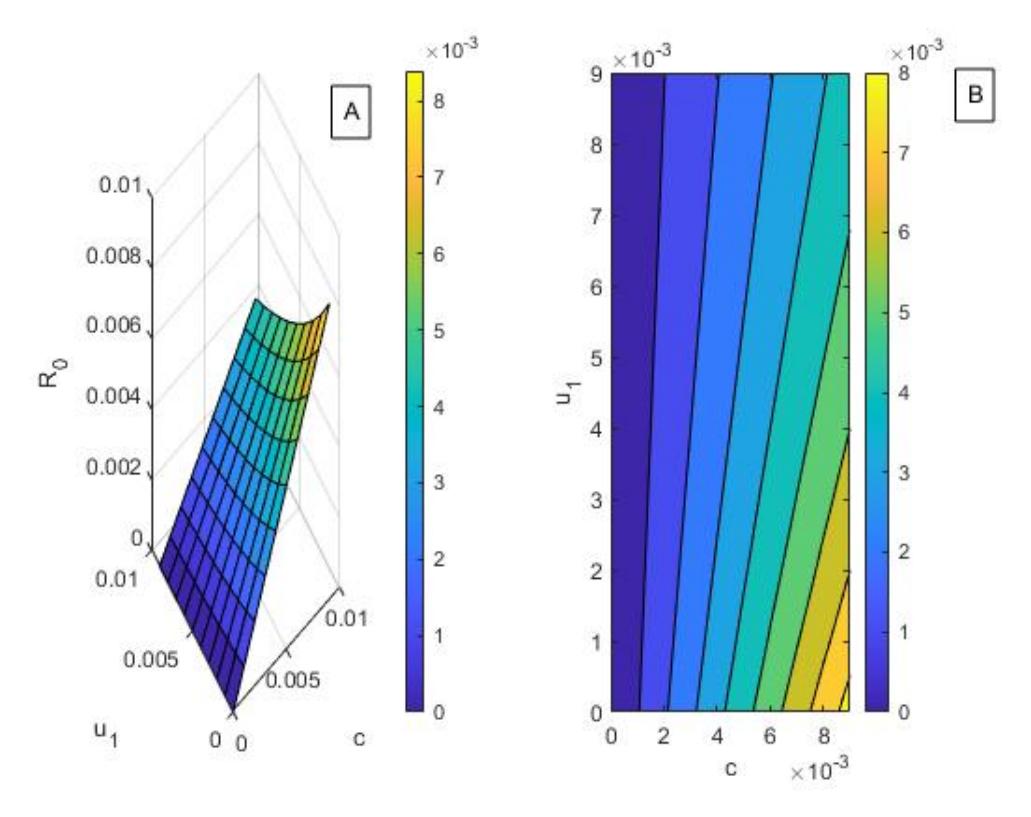
Figure 6.33: (A) the dependence of basic reproduction number on per capita contact rate c and vaccination control u1. (B) represents the contour plot for the Figure (A).
and vaccination is the most effective way to minimize infection, maximize the recovery rate and after all to control the progression of the disease. As a part of future work, to apply optimal control strategy by using second order ODE would be appreciated with the change of optimality condition. In the modern day's HIV and TB are top at the list of infectious diseases worldwide. So, to eradicate or to minimize these kinds of contagious diseases is the gigantic challenge through the world. In the age of modern science and technology the oppression of HIV and TB is not expectable. So proper program for HIV -TB, to create opportunity for reaches on HIV-TB and create awareness among the mass population can be helpful to control the infections rate. Counseling for HIV-TB co-infected persons to a great extent, availability of treatment and antidote, early detection of HIV-TB and plan to reduce the virus transmission should be emphasized. The government and the infectious diseases institutes should take all round steps against HIV and TB to eliminate this curse from the human planet.
ACKNOWLEDGMENT
This research is partially supported with the grant ref. no.-39.00.0000.009.06.024.19-12/EAS-410 under special allocations funded by the Ministry of Science and Technology, Government of the People's Republic of Bangladesh, 2019-2020.