

1. INTRODUCTION
Dengue disease is the most common mosquito-borne disease in the world, especially in tropical and subtropical countries [1]. This disease is transmitted by Aedes aegypti and Aedes albopictus [2] which carry the dengue virus, where Aedes aegypti is a mosquito species that is highly adapted to human habitats [3]. There are four serotypes of the dengue virus, that is, DENV-1, DENV-2, DENV-3 and DENV-4 [4], [5]. Dengue infection can cause classical dengue fever (DF), such as asymptomatic or mild symptoms, dengue hemorrhagic fever (DFF) and dengue shock syndrome (DSS) [6].
Dengue is a global health threat because of its high prevalence, limited vaccines and prevention efforts, and lack of specialized care. Dengue disease has been known for more than three centuries, but the antiviral drugs and vaccines, that are currently under development, are still relatively expensive and not even widely marketed. Therefore, the only effort recommended by WHO to prevent dengue disease is intervention to control mosquito population growth. The control of mosquito population can be done through environmental management and chemical control (larvicides). Environmental management includes improvement of water supply and water-storage systems, using mosquito-proofing of water storage containers, solid waste management, street cleansing, and improving planning and construction of buildings and other infrastructure [7]. In addition, the control and prevention of dengue transmission can be done biologically [8]. In general, the dengue disease prevention and control strategy established by the resolution SEA/RC61/R5 of the WHO Regional Committee for Southeast Asia in 2008, consists of six elements, namely: (i) dengue data collection (surveillance); (ii) case management; (iii) outbreak management or response; (iv) integrated vector management; (v) social mobilization and communication for dengue; and (vi) research on dengue [9].
Efforts to prevent and control dengue disease through qualitative and quantitative research strategies have been widely reported, using deterministic and stochastic models, or a combination of the two models. Several
*Corresponding author
Received June 2nd, 2022, Revised June 15th, 2022, Accepted for publication June 30th, 2022. Copyright ©2022 Published by Indonesian Biomathematical Society, e-ISSN: 2549-2896, DOI:10.5614/cbms.2022.5.1.5
studies have used deterministic models to understand dengue transmission, such as a model with constant human and vector populations [10], a model involving asymptomatic individuals [11], and a two-age-classes model with vaccination [12]. Meanwhile, the studies in [13] used stochastic approaches to study dengue disease transmission. Otero and Solari [13] stated that the dynamics of dengue disease was triggered by the arrival of infected people in a city. They also stated that the probability of an epidemic outbreak depended on seasonal variation in temperature and availability of breeding sites. Other studies even compare deterministic and stochastic models to understand dengue disease transmission, such as in Bandung, Indonesia [14] and Kampong Cham, Cambodia [15]. Furthermore, there is a growing concern about the possible increase in dengue transmission as a result of the influence of climatic factors, prompting many empirical studies to investigate the relationship of climate to dengue disease. The empirical study uses various analytical approaches, such as correlation, cross-correlation, automatic correlation, and time series regression models [16], [17]. In particular, the nonlinear relationship between climate and dengue disease considering the effect of temperature lag on dengue disease transmission was studied in [18], [19]. Moreover, Chen et al. [20] performed a Poisson regression analysis using the generalized estimating equations (GEE) approach to examine the potential effects of climate variations on the epidemiological pattern of dengue in Taiwan during 2001 − 2008. The best model was selected based on the quasi-likelihood based information criterion (QICu). The combination of the Poisson time series model and the distributed lag model (DLM) to estimate the impact of weather on dengue disease transmission in Dhaka, Bangladesh has also been introduced by Bhanu et al. [21]. Furthermore, Fakhrudin et al. [22] constructed a multi-clustering multiple regression model to predict the incidence of dengue disease based on rainfall and humidity data. Rainfall and relative humidity were associated with the daily incidence of dengue at 8-week interval.
In this study, we conducted a Poisson regression analysis that linked climate factors with the incidence of dengue disease in Bandung city based on daily, weekly, and monthly data. In contrast to previous studies, the novelty of this study is to integrate external factors, namely dynamic climate factors with dynamic models of dengue transmission. In this case, the regression estimation results in the form of the average number of infected human population are used as a database to estimate the proportion infected human for the short term (one period ahead) through a different equation approach. Based on the estimation result of the proportion of infected human, we then estimate the proportion of infected mosquitoes using a quasi steady state (QSS) approach. Finally, we estimate the proportion of infected human and infected mosquito over the long term using a deterministic and stochastic differential approach.
2. MATERIAL AND METHODS
2.1. Data Collection
In this study, we used daily dengue data from Santo Boromeus Hospital, Bandung city. Furthermore, climate data was taken from the Meteorology, Climatology and Geophysics Agency (MCGA) Bandung, from 2009 to 2017 [23]. The climate factors used in this study were the volume of rainfall, relative humidity, minimum temperature, maximum temperature, average temperature, duration of irradiation, average wind speed and maximum wind speed. Next, we explored daily dengue incidence data into total infection data for daily, weekly, and monthly time periods. Bandung city Health Office reported that 37,284 people or 50.59% of the total dengue disease patients in Bandung city were treated at the Santo Boromeus Hospital [24]. Therefore, in this study, we use a population size of 50% of the total population of Bandung city.
The number of daily incidences of dengue disease in Bandung city fluctuates every day, as shown in Figure 1. There is a significant difference between the quantity of new cases of dengue disease and the total number of dengue patients in the hospital. The highest new incidence of dengue occurred in 2009 and the lowest in 2017. The incidence of dengue in Bandung city generally peaked on May and lowest on October. The results of this observation are relatively different from the results of observations in previous studies [25], [26]. Esteva and Yang [25] stated that the incidence of dengue in Yucatan, Mexico, during 2009-2011 occurred at the end of the rainy season, which is around October and November. Meanwhile, Zhu and Xu [26] suggested that the incidence of dengue generally peaks on June, July, and August. This indicates that different regions may have different times of peak incidence of dengue.
2.2. Statistical Analysis
Here, we performed a cross-correlation analysis to characterize the relationship between the number of human infected and climate factors, either for daily, weekly, or monthly time periods. The time lag is
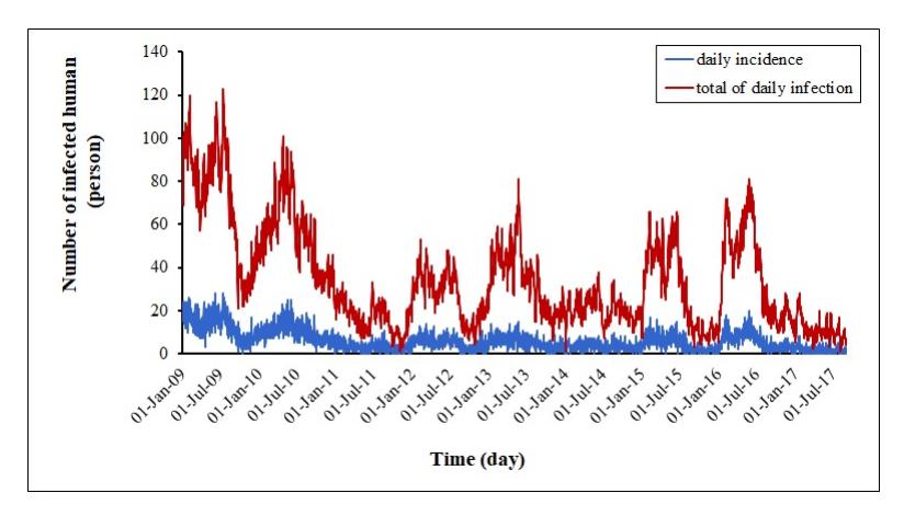
Figure 1: Number of infected human in Bandung city, from January 2009 to 31 August 2017.
determined based on the dominant coefficient values of all climate factors. Let X1,t−p, X2,t−p, X3,t−p, X4,t−p, X5,t−p, X6,t−p, X7,t−p, and X8,t−p denote the climate variables consisting of rainfall, relative humidity, minimum temperature, maximum temperature, average temperature, duration of irradiation, average wind speed, and maximum wind speed, for p−lag at time t, respectively. While, X9,t−2 and X10,t−1 denote the history of dengue incidence, that are, the number of infected human for 2−lag and 1−lag at time t, respectively.
Furthermore, we performed a regression analysis. In this study, we assume that the number of infected human (IH,t) follows a Poisson distribution, with the mean µH,t, which can be written as
\[I_{H,t} \sim Poisson(\mu_{H,t}),\] (1)
where E(IH,t) = µH,t. The average number of infected human for each time period is defined by
\[\mu_{H,t} = e^{(X_t^T \beta)},\tag{2}\]
where β = (β0, β1, ..., β10) T and Xt = (1, X1,t−p, ..., X8,t−p, X9,t−2, X10,t−1) T . To obtain a consistent regression model, we divided the data into two groups, i.e., 70% of the data was used as training data and 30% of the data was used as testing data. Furthermore, we would consider removing climate variables that are not statistically significant to increase the model's accuracy. The best regression model was determined based on the union of mean square error (UMSE) value from the training and testing data. The UMSE value is calculated using the following equation:
\[UMSE = \frac{1}{2}(MSE_{training\ data} + MSE_{testing\ data}). \tag{3}\]
Next, we use the best regression model of Equation (2) to approximate the proportion of infected human, which is written in the following formula:
\[\bar{I}_{H,t} \approx \frac{\mu_{H,t}}{N_H},\tag{4}\]
where NH is the number of infected human population. The estimation results obtained from Equation (4) are then used as a database for analyzing the dynamics of dengue disease transmission.
2.3. Deterministic Model of Dengue Disease Transmission and Its Analysis
Estimates of the proportion of infected human will be analyzed based on the dynamic of dengue disease transmission model introduced by Esteva and Vargas in [10], [27]. In this study, we use Equation (4) to estimate the proportion of infected human using a different equation approach. Thus, the influence of climate factors on the dynamics of dengue transmission is inclusively included in the model. We assume that the human and mosquito populations are constant. Here, the human population is composed of three sub-populations: the susceptible \((S_{H,t})\), the infected \(I_{H,t}\), and the recovered \(R_{H,t}\), at time t. While, the vector population is divided two sub-populations: the susceptible \((S_{V,t})\) and the infected \(I_{V,t}\), at time t. The dynamic of dengue disease transmission in this study is written in the following deterministic model.
\[\frac{dS_{H,t}}{dt} = \nu_{H} N_{H} - \lambda_{H} S_{H,t} \frac{I_{V,t}}{N_{V}} - \nu_{H} S_{H,t}, \frac{dI_{H,t}}{dt} = \lambda_{H} S_{H,t} \frac{I_{V,t}}{N_{V}} - (\nu_{H} + \gamma_{H}) I_{H,t}, \frac{R_{H,t}}{dt} = \gamma_{H} I_{H,t} - \nu_{H} R_{H,t}, \frac{dS_{V,t}}{dt} = \nu_{V} N_{V} - \lambda_{V} S_{V,t} \frac{I_{H,t}}{N_{H}} - \nu_{V} S_{V,t}, \frac{dI_{V,t}}{dt} = \lambda_{V} S_{V,t} \frac{I_{H,t}}{N_{H}} - \nu_{V} I_{V,t},\] (5)
where \(N_{H,t}\) and \(N_{V,t}\) represent the total populations of human and mosquito, respectively. The effective contact rates, i.e., \(\lambda_H\) and \(\lambda_V\), are the average number of contacts per day that effectively transmit the infection to human and mosquitoes, which are formulated as \(\lambda_H = b\varphi_H \kappa\) and \(\lambda_V = b\varphi_V\), respectively. Descriptions of other model parameters are presented in Table 1, where all parameters of Model (5) are nonnegative. This means that if the initial data \((S_{H,t}, I_{H,t}, R_{H,t}, S_{V,t}, I_{V,t})\) is in \(R_+^5\) region, then the solution will be defined for all time \(t \geq 0\) and stay in this region [28]. The subset \(\Omega\), defined by \(S_{H,t} + I_{H,t} + R_{H,t} = N_{H,t}\) and \(S_{V,t} + I_{V,t} = N_{V,t}\), is region invariant for Model (5), because any solution starting at \(\Omega\) satisfies \(N'_{H,t} = 0\) and \(N'_{V,t} = 0\). Human and mosquito populations remain constant at \(\Omega\). So, the proportion of each variable in the model (5) is defined as follows:
\[\bar{S}_{H,t} = \frac{S_{H,t}}{N_{H,t}}, \bar{I}_{H,t} = \frac{I_{H,t}}{N_{H,t}}, \bar{R}_{H,t} = \frac{R_{H,t}}{N_{H,t}}, \bar{S}_{V,t} = \frac{S_{V,t}}{N_{V,t}}, \bar{I}_{V,t} = \frac{I_{V,t}}{N_{V,t}}.\]
Therefore, Model (5) can be written in the form of proportions as follows:
\[\frac{d\bar{S}_{H,t}}{dt} = \nu_H - \lambda_H \bar{S}_{H,t} \bar{I}_{V,t} - \nu_H \bar{S}_{H,t},\] \[\frac{d\bar{I}_{H,t}}{dt} = \lambda_H \bar{S}_{H,t} \bar{I}_{V,t} - (\nu_H + \gamma_H) \bar{I}_{H,t},\] \[\frac{d\bar{R}_{H,t}}{dt} = \gamma_H \bar{I}_{H,t} - \nu_H \bar{R}_{H,t},\] \[\frac{d\bar{S}_{V,t}}{dt} = \nu_V - \lambda_V \bar{S}_{V,t} \bar{I}_{H,t} - \nu_V \bar{S}_{V,t},\] \[\frac{d\bar{I}_{V,t}}{dt} = \lambda_V \bar{S}_{V,t} \bar{I}_{H,t} - \nu_V \bar{I}_{V,t}.\] (6)
If \(\bar{R}_{H,t}=1-\bar{S}_{H,t}-\bar{I}_{H,t}\) and \(\bar{S}_{V,T}=1-\bar{I}_{V,t}\), then Model (6) can be written as a three-dimensional nonlinear system as follows:
\[\frac{d\bar{S}_{H,t}}{dt} = \nu_H (1 - \bar{S}_{H,t}) - \lambda_H \bar{S}_{H,t} \bar{I}_{V,t}, \tag{7}\]
\[\frac{d\bar{I}_{H,t}}{dt} = \lambda_H \bar{S}_{H,t} \bar{I}_{V,t} - (\nu_H + \gamma_H) \bar{I}_{H,t}, \tag{8}\]
\[\frac{d\bar{I}_{V,t}}{dt} = \lambda_V (1 - \bar{I}_{V,t}) \bar{I}_{H,t} - \nu_V \bar{I}_{V,t}. \tag{9}\]
Furthermore, the basic reproduction number \((R_0)\) is constructed using the next generation matrix method in [34], which is evaluated at the disease-free equilibrium point \(E_0 = (1, 0, 0)\). The basic reproduction number
| Parameter | Description | Value | Dimension | Reference |
|---|---|---|---|---|
| \(\nu_H\) | Birth or death rates of human per unit time | \(1/(70 \times 365)\) | \(day^{-1}\) | [29] |
| \(\nu_V\) | Birth or death rates of mosquito per unit time | 0.25 | \(day^{-1}\) | [10] |
| b | Average bites per mosquito per unit time | 0.33 | \(day^{-1}\) | [30], [31] |
| \(\kappa\) | Ratio between mosquito and human population | 3 | _ | Assumed |
| \(\varphi_H\) | Probability of transmission from infected mosquito to susceptible human | 0.33 | _ | [21], [32], [33] |
| \(\varphi_V\) | Probability of transmission from infected human to susceptible mosquito | 0.33 | _ | [21], [32], [33] |
| \(\gamma_H\) | Human recovery rate | 1/7 | \(day^{-1}\) | [10] |
Table 1: Parameter model description and value.
corresponding to the equations (7)-(9) is formulated as follows:
\[R_0 = \sqrt{\frac{\lambda_H}{\nu_V} \frac{\lambda_V}{(\nu_H + \gamma_H)}}. (10)\]
This \(R_0\) is a threshold condition for determining global dynamic behavior. If \(R_0 < 1\) then there will be a global stable disease-free equilibrium, i.e. the disease will be extinct. On the other hand, if \(R_0 > 1\) then a globally stable unique endemic equilibrium occurs. This means that the disease will always remain endemic above the threshold value [34], [35]. In Equation (10), the first ratio under the square root, i.e., \(\frac{\lambda_H}{\nu_V}\), represents the number of mosquito infections caused by one infected human, and the second, i.e., \(\frac{\lambda_V}{\nu_H + \nu_H}\), represents the number of human infections caused by one infected mosquito [34], [35].
Here, we also construct the reproduction number at time t (\(R_t\)) since the start of the epidemic which is defined as effective reproduction number [36]. The effective reproduction number of equation (7)-(9) as proposed by [35] is
\[R_t = R_0 \sqrt{\frac{\bar{S}_{H,t} (1 - \bar{I}_{V,t}) \nu_V}{\lambda_V \bar{I}_{H,t} + \nu_V}}.\] (11)
Estimation of the proportion of infected mosquito per unit time cannot be carried out directly using Equation (7)-(9), because the mosquito population is unobserved. The mosquito life span is relatively short compared to the human life span, which is about 15 to 45 days. Thus, we assume that the change in the infection rate in mosquito is \(\frac{d\bar{I}_{V,t}}{dt} \to 0\), for \(t \to \infty\). By applying the Quasi Steady State (QSS) method to Equation (7)-(9), we get an approximate value of the proportion of infected mosquito at time t, which can be written as follows:
\[\bar{I}_{V,t} = \frac{\lambda_V \bar{I}_{H,t}}{\lambda_V \bar{I}_{H,t} + \nu_V}.\] (12)
If Equation (12) is substituted into the equation (7) and (8), then we obtain
\[\frac{d\bar{S}_{H,t}}{dt} = \nu_H (1 - \bar{S}_{H,t}) - \lambda_H \bar{S}_{H,t} \frac{\lambda_V \bar{I}_{H,t}}{\lambda_V \bar{I}_{H,t} + \nu_V}, \tag{13}\]
\[\frac{d\bar{I}_{H,t}}{dt} = \lambda_H \bar{S}_{H,t} \frac{\lambda_V \bar{I}_{H,t}}{\lambda_V \bar{I}_{H,t} + \nu_V} - (\nu_H + \gamma_H) \bar{I}_{H,t}. \tag{14}\]
If we assume that \(\bar{R}_{H,t}\) is very small, \(\bar{R}_{H,t} \approx 0\), then \(\bar{S}_{H,t} = 1 - \bar{I}_{H,t}\). Therefore, Equation (14) is written as
\[\frac{d\bar{I}_{H,t}}{dt} = \lambda_H (1 - \bar{I}_{H,t}) \frac{\lambda_V \bar{I}_{H,t}}{\lambda_V \bar{I}_{H,t} + \nu_V} - (\nu_H + \gamma_H) \bar{I}_{H,t}, \tag{15}\]
Furthermore, we use a numerical approach to solve the ordinary differential equation (15).
2.4. Stochastic Model
In this study, the approximate numerical solution of Equation (15) is determined using the Euler method, which is written in the following formula.
\[\bar{I}_{H,t+1} = \bar{I}_{H,t} + \Delta t \left( \lambda_H (1 - \bar{I}_{H,t}) \frac{\lambda_V \bar{I}_{H,t}}{\lambda_V \bar{I}_{H,t} + \nu_V} - (\nu_H + \gamma_H) \bar{I}_{H,t} \right), \tag{16}\]
where \(\bar{I}_{H,t}\) is Poisson distributed with rate \(\mu_{H,t}\). Here, we need to calculate the average number of infected human associated with the climate factors, \(\mu_{H,t}\), using the best regression model of Equation (2). Next, we generate a random number from the Poisson distribution specified by the parameter \(\mu_{H,t}\) and approximate the proportion of infected human at time t, \(\bar{I}_{H,t}\), using the equation (4). This procedure was carried out a thousand times to obtain a 95% confidence interval for the estimation results. The confidence interval is obtained by sorting the simulation results and taking the 2.5% value from the top and bottom of the sorting results.
3. RESULT AND DISCUSSION
3.1. Association of climate Factors and Dengue Incidence
1) Bivariate Correlation between Climate Factors and Dengue Incidence: To perform cross-correlation analysis one needs to measure first the bivariate correlation between climate factors and dengue incidence for daily, weekly, and monthly time periods without any time lag. Pearson's correlation coefficient, Spearman's rho, and Kendall's tau-b with their significance levels are presented in Table 2. The results confirmed the fact that not all climate factors are positively and significantly associated with the dengue incidence. Rainfall factor in daily, weekly, and monthly time periods are not significantly associated with the dengue incidence. This is different from the results in studies [25], [37] which stated that dengue disease is associated with rainfall intensity. The minimum temperature factor was significantly associated with daily dengue incidence, but was not associated with weekly and monthly dengue incidence. Meanwhile, relative humidity was positively and significantly associated with the incidence of dengue. Furthermore, maximum temperature, average temperature, duration of irradiation, average wind speed, and maximum wind speed per day were negatively associated with dengue incidence.
| Pearson | Kendall's Tau-b | Spearman's rho | |||||||
|---|---|---|---|---|---|---|---|---|---|
| D | W | M | D | W | M | D | W | M | |
| \(r_{X_1I_H}\) | 0.004 | 0.011 | 0.016 | 0.012 | 0.041 | 0.035 | 0.017 | 0.062 | 0.060 |
| \(r_{X_2I_H}\) | 0.237** | 0.295** | 0.332** | 0.166** | 0.214** | 0.225** | 0.240** | 0.310** | 0.331** |
| \(r_{X_3I_H}\) | 0.036* | 0.044 | 0.061 | 0.032* | 0.045 | 0.043 | 0.047** | 0.067 | 0.066 |
| \(r_{x_4I_H}\) | -0.142** | -0.201** | -0.235* | -0.109** | -0.131** | -0.147* | -0.160** | -0.192** | -0.214* |
| \(r_{X_5I_H}\) | -0.111** | -0.160** | -0.192 | -0.070** | -0.105** | -0.174** | -0.105** | -0.155** | -0.256** |
| \(r_{X_6I_H}\) | -0.067** | -0.134 | -0.122 | -0.050** | -0.082** | -0.081 | -0.075** | -0.122** | -0.123 |
| \(r_{X_7I_H}\) | -0.143** | -0.177** | -0.216* | -0.101** | -0.095** | -0.118 | -0.126** | -0.132** | -0.168 |
| \(r_{X_8I_H}\) | -0.116** | -0.188** | -0.241* | -0.078** | -0.131** | -0.190** | -0.103** | -0.185** | -0.265** |
Table 2: Correlation coefficient for Pearson, Kendall's Tau, and Spearman's rho.
The results of the cross-correlation analysis are presented briefly in Figure 2. Figure 2 shows that the number of dengue incidences is significantly related to climate factors, with a certain time lag. The most dominant time lags that give a higher correlation coefficient value for daily, weekly, and monthly time periods are 60 days, 8 weeks, and 2 months, respectively. From Figure 2, we know that climate factors consisting of rainfall, relative humidity, minimum temperature, maximum temperature, duration of irradiation, average wind speed, and maximum wind speed are significantly associated with an increase in dengue incidences at these time lags.
** Correlation is significant at the 0.01 level (2-tailed)
* Correlation is significant at the 0.05 level (2-tailed)
D = Daily, W = Weekly, M = monthly
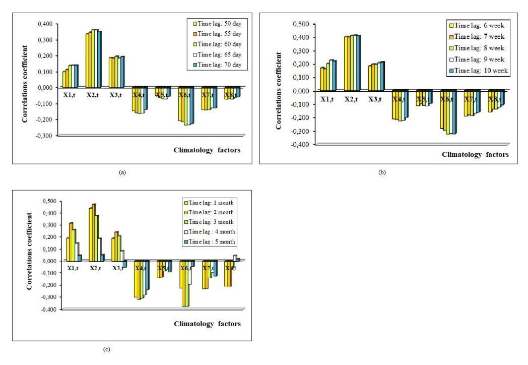
Figure 2: Cross-correlation between the number of infected human and climate factors: (a) lag in day, (b) lag in week (c) lag in month.
2) The Influence of Climate Factors on the Dengue Incidence: We found that the historical incidences of dengue disease and climate factors with a time lag of 60-days or 8-weeks or 2-months influenced the development of the dynamics of dengue disease transmission at time t. The best regression model based on daily, weekly, and monthly data are written in the following equations.
\[\mu_{H,t} = \exp(1.3821 + 0.0075X_{2,t-60} + 0.0038X_{3,t-60} + 0.0046X_{5,t-60} + 0.0017X_{9,t-60} + (17) \\ 0.0238X_{10,t-1}),\]
\[\mu_{H,t} = \exp(1.1807 + 0.0101X_{2,t-8} + 0.0169X_{3,t-8} + 0.0102X_{4,t-8} - 0.0241X_{5,t-8} + 0.0095X_{9,t-8} + 0.0140X_{10,t-1}),\] (18)
\[\mu_{H,t} = \exp(2.6513 + 0.0056X_{1,t-2} + 0.0227X_{3,t-2} + 0.0168X_{4,t-2} - 0.0264X_{5,t-2} + 0.0059X_{8,t-2} + 0.0215X_{10,t-1}),\] (19)
where µH,t represents the estimated average number of infected human, with the MSE values for each equation are 56.47, 140.62, and 2.88 × 10³ , respectively.
The regression model that we present in Equation (17)-(19) confirms the fact that the climate factors contribute to increasing the average number of infected human for each time period, which are 31.57% per day, 53.46% per week, and 17.48% per month, respectively. In detail, the regression model for daily data, i.e., Equation (17), provides information that the climate factors that influence the dengue incidence in Bandung city are relative humidity, minimum temperature, and average temperature, with the dominant factor is relative humidity. However, in the regression model for weekly data, Equation (18), the maximum temperature also affects the dengue incidence. In this model, the dominant factor is average temperature factor. Meanwhile, from the regression model for monthly data, Equation (19), rainfall, temperature (minimum, maximum, and average) and maximum wind speed are climate factors that affect dengue incidence in Bandung city, with the dominant factor is the average temperature. These results is slightly different with the study of [18], which reported that there was a positive relationship between maximum temperature and relative humidity, and the
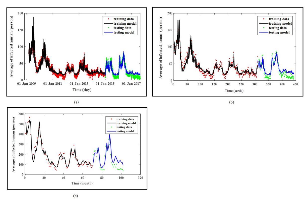
Figure 3: Estimated average number of infected human population, based on: (a) daily data; (b) weekly data; and (c) monthly data.
incidence of dengue, with 2-month lag time. Furthermore, the estimation results in Equation (17)-(19) can be described in graphical form as shown in Figure 3. From Figure 3, it can be seen that the estimation model is close to the actual data on dengue incidence in Bandung city.
3.2. Dynamics of Dengue Disease Transmission
Using the regression models (17)-(19), we are now able to plot the dynamic of proportion of infected human \((\bar{I}_{H,t})\) in Equation (16) for daily, weekly, and monthly time periods, as shown in Figures 4 (a), (c) and (e). The values of the parameters involved in the model can be seen in Table 1, where the values are multiplied by 7 for weekly data and 30 for monthly data. From this computation, the proportion of infected mosquito \((\bar{I}_{V,t})\) in Equation (12), susceptible human, with \(\bar{S}_{H,t}=1-\bar{I}_{H,t}\), and susceptible mosquito, with \(\bar{S}_{V,t}=1-\bar{I}_{V,t}\), can also be obtained as presented in Figure 4. This proportion is determined by assuming that the mosquito population \((N_V)\) is equal to three times the total human population, where \(N_H=1,250,000\). From Figures 4 (a), (c) and (e), it is known that the proportion of infected human is much greater than the proportion of infected mosquito. The value of the proportion of infected human that is greater than the proportion of infected mosquito cannot be analogized directly that the number of infected human population is greater than the number of infected mosquito population. Figure 4 also shows that the proportion of infected mosquitoes per day ranged from 0.46 to 6.77 per 100,000, with an average of 1.17 per 100,000. Based on weekly data, the proportion of infected mosquito ranged from 0.56 to 5.96 per 100,000, with an average of 1.44 per 100,000. Meanwhile, in monthly data, the proportion of infected mosquito ranged from 2.81 to 24.77 per 100,000, with an average of 6.58 per 100,000.
In order to provide a range of plausible values for the estimated proportion of infected human, we performed a thousand simulations and took a 95% confidence interval as shown in Figure 5. Here, we also present the
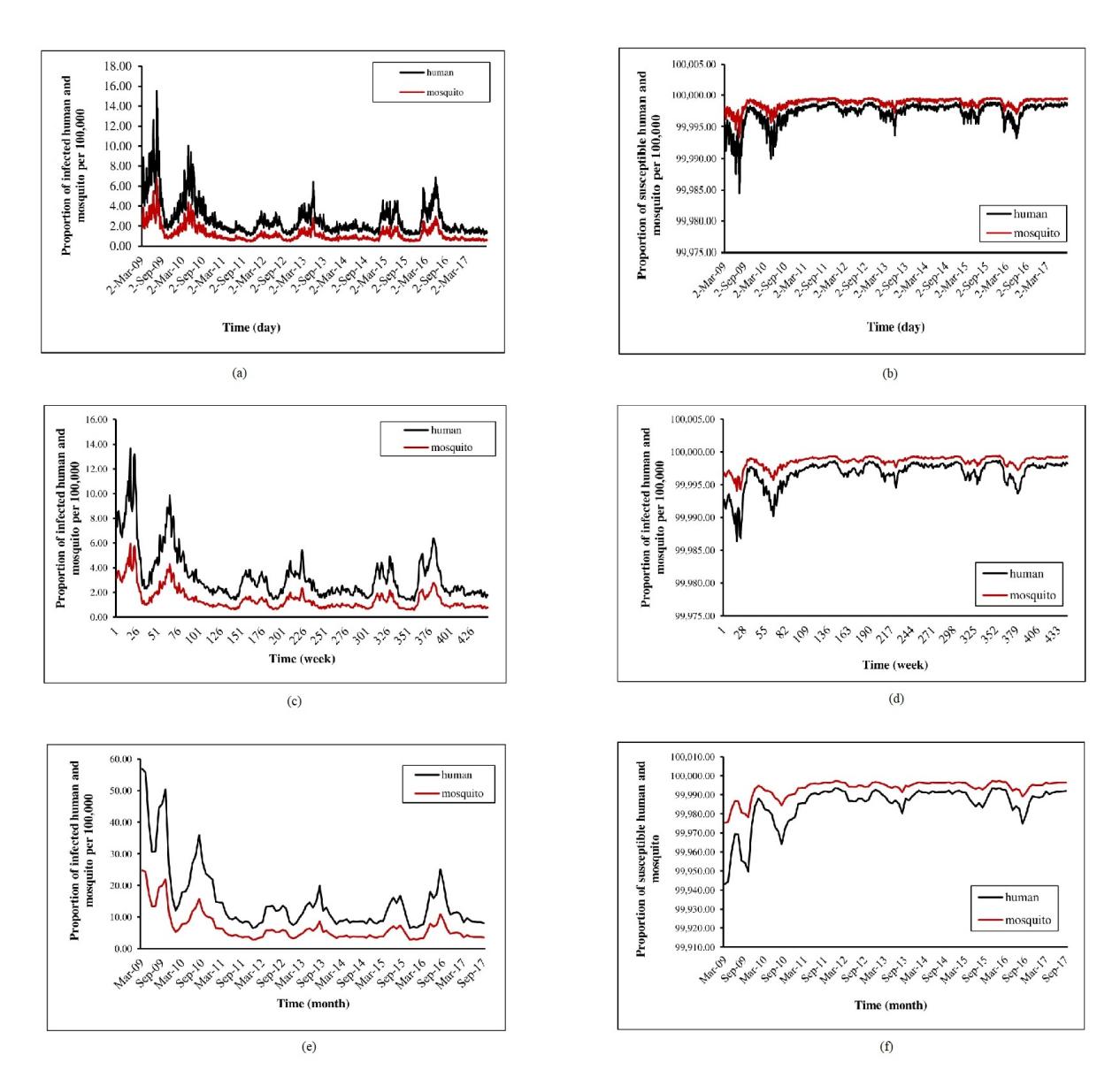
Figure 4: Proportion of infected human and mosquito for (a) daily data; (b) weekly data; (c) monthly data; and the proportion of susceptible human and mosquito for (d) daily data; (e) weekly data; (f) monthly data.
numerical solution of deterministic model (15) using the initial condition of \(\bar{I}_{H,0}\): \(7.248 \times 10^{-5}\) for daily data; \(7.325 \times 10^{-5}\) for weekly data; \(4.157 \times 10^{-4}\) for monthly data, and the parameter value in Table 1, as can be seen in Figure 5. From Figure 5, it can be seen that the stochastic model is closer to the actual data than the deterministic model.
In Figure 6, we plot the effective reproduction number \((R_t)\) using Equation (11) and the solution of stochastic model, based on daily, weekly, and monthly data. The \(R_t\) number is a threshold for characterizing the dynamics of transmission and measuring the effectiveness of dengue transmission control at time t. The \(R_t\) values in Figure 6 are below the threshold \((R_t = 1)\), although quite a lot of \(R_t\) values are close to the
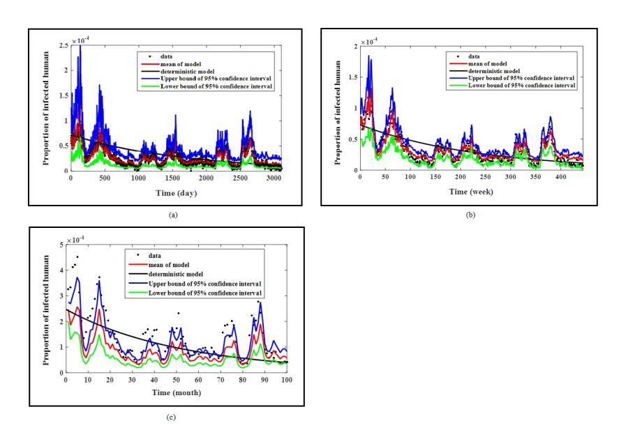
Figure 5: Simulation of deterministic and stochastic models based on: (a) daily data; (b) weekly data; and (c) monthly data.
threshold. This indicates that dengue disease transmission in Bandung city from 2009 to 2017 can generally be controlled quickly. However, there are some time intervals for dengue disease control which are quite slow, that is, when the threshold value of Rt is close to 1. At this time interval indicates that dengue transmission control is less effective, although the increase in dengue transmission is extreme, i.e. towards an endemic condition or not free from disease.
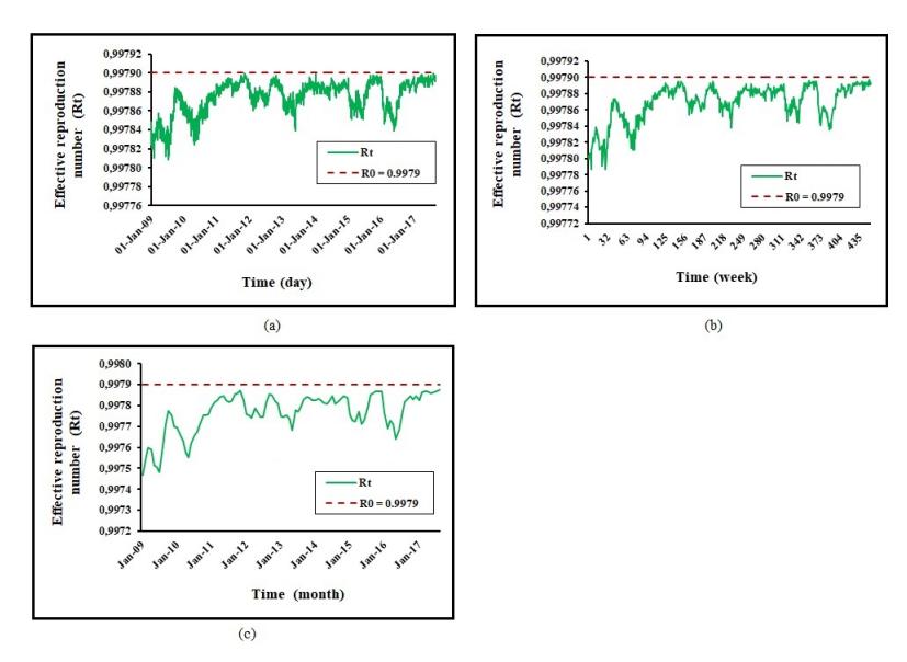
Figure 6: Effective reproduction number based on: (a) daily data; (b) weekly data; and (c) monthly data.
Overall, from the simulation results of deterministic and stochastic models, the stochastic model gives more representative estimation results than the deterministic model. The estimation results obtained using daily, weekly, and monthly data show a relatively similar trend. Lastly, we observed that estimates with daily data give better results than estimates with weekly or monthly data.
4. CONCLUSION
In this study, we show that climate factors contribute to the increasing dengue incidence in Bandung city, based on daily, weekly, and monthly data from 2009 to 2017. The dominant factors that most influence the dynamics of dengue disease transmission are relative humidity for daily data and average temperature for weekly and monthly data. We also found that the dynamical model was quite effective in estimating the proportion of infected human and mosquito, both with deterministic and stochastic approaches. The stochastic model is more representative than the deterministic model in estimating the proportion of infected human and mosquito population. By knowing the proportion of infected mosquito, we can control and reduce the spread of dengue.
ACKNOWLEDGEMENT
Part of the work of the author JWP is funded by the Indonesian Penelitian Disertasi Doktor Kemdikbudristek 2022 (No: 5R/IT1.C02/TA.00/2022).