

1. Introduction
There has been a growing interest in the study of genetic variation in the populations. It is very much essential to know how genetic variation in the population affects ecological process as well as the outcome of interacting species. The idea of ecogenetics is similar to eco-epidemiological systems, in which instead of infected and susceptible individuals, the two subgroups of a population is divided are different from their distinct genetic structures and traits. The study of ecogenetics indicates in what way acquired genetic variation behaves to atmospheric changes, such as substances exist in it [1], [2]. Venturino [3] introduced the concept of ecogenetics in a predator-prey system where prey is genetically differentiated. Further, this idea is employed in predator population [4]. In [4], the authors remarked that the system does not admit persistent oscillations. The model studied in [4] further modified by incorporating Holling type II response function [5]. Wang and Zhao [6] studied a predator-prey model considering the genetic variation in both the populations. Astles et al. [7] pointed out genetic variation in ladybird predator. It is observed that trait variation in the predator allows prey species to coexist and in some situation even reveal beneficial. So abrupt changes in outcomes recommend that studies which overlook trait variation may reach basically wrong inferences [8]. So, it is reasonable to investigate the effect of genetic modification in predator population on the ecosystem.
In [4], the authors investigated the dynamical behaviour of the following model:
\[\frac{dx}{d\tau} = R(1 - \frac{x}{K})x - hxy - gxz,\] \[\frac{dy}{d\tau} = pe(hy + gz)x - my,\] \[\frac{dz}{d\tau} = qe(hy + gz)x - nz,\] (1)
where \(x(\tau)\) stands the prey population and \(y(\tau)\) and \(z(\tau)\) represent the two genotypes of the predators, functions of time \(\tau\). Moreover, R stands for the per capita net prey reproduction rate, K is the environmental carrying capacity of prey, m and n are the natural death rate of the two predators' genotypes y and z. h and g denote hunting rates for the predator y and z. 0 < e < 1 denote the conversion efficiency of the predators. p and q = 1 - p represent the fractions of predators' newborns respectively of genotype y and z. All the parameters are taken as nonnegative.
By using the suitable transformations the model (1) becomes:
\[\frac{dX}{dt} = r(1-X)X - cXY - XZ, \frac{dY}{dt} = w(cY+Z)X - sY, \frac{dZ}{dt} = v(cY+Z)X - dZ,\] (2)
where \(w=pgK, v=qgK, r=\frac{R}{e}, c=\frac{h}{g}, s=\frac{m}{e}, d=\frac{n}{e}\). It is a natural fact that discrete time models represented by difference equations are more reasonable than the continuous time models when populations have non-overlapping generations [9], [10]. For example, discrete time is appropriate to introduce in some models of fish population, which reproduce at specific time moments, or for insect population, for which very often non-overlapping generations are found in nature [11].
By analytical studies, it is noted that the discrete time models have various properties and structures in comparison to continuous systems. Such systems describing discrete models are investigated in [12], [13], [14], [15], [16], [17], [18]. The above discussions motivate us to investigate the discrete version of System (2). The discrete model corresponding to System (2) is:
\[X_{n+1} = r(1 - X_n)X_n - cX_nY_n - X_nZ_n,\] \[Y_{n+1} = w(cY_n + Z_n)X_n - sY_n,\] \[Z_{n+1} = v(cY_n + Z_n)X_n - dZ_n.\] (3)
The paper is structured as follows. The existence and the nature of the positive fixed point are examined in Section 2. Neimark-Sacker bifurcation is described in Section 3. Chaos control is demonstrated in Section 4. Examples are given in Section 5. Section 6 ends the paper with a discussion.
2. EXISTENCE OF INTERIOR FIXED POINT
System (3) allows only two nontrivial fixed points, in addition to the origin \(E_0 = (0,0,0)\), namely the predator free fixed point \(E_1 = (\frac{r-1}{r}, 0, 0)\), which is feasible when r > 1 and the interior fixed point \(E^* = (X^*, Y^*, Z^*)\) whose components can be explicitly determined in the following proposition.
Proposition 1. System (3) has a unique interior fixed point \(E^* = (X^*, Y^*, Z^*)\) if
\[r > \frac{cw(1+d) + v(1+s) + r(1+s)(1+d)}{cw(1+d) + v(1+s)}\]
Proof: The fixed point can be determined by simple calculations of the system given below:
\[\begin{array}{rcl} X^* & = & X^*\{r(1-X^*)-cY^*-Z^*\}, \\ Y^* & = & w(cY^*+Z^*)X^*-sY^*, \\ Z^* & = & v(cY^*+Z^*)X^*-dZ^*. \end{array}\]
Ignoring the boundary fixed points, we have
\[1 = r(1 - X^*) - cY^* - Z^*, (4)\]
\[Y^* = w(cY^* + Z^*)X^* - sY^*, (5)\]
\[Z^* = v(cY^* + Z^*)X^* - dZ^*. (6)\]
From Equation (4), we get \(Z^*=r(1-X^*)-cY^*-1\). By using this value of \(Z^*\) in (5), we have \(Y^*=\frac{wX^*\{r(1-X^*)-1\}}{1+s}\). Eliminating \(Y^*\) from (4) and (6), we get \(Z^*=\frac{vX^*\{r(1-X^*)-1\}}{1+d}\). Now putting the expression for \(Y^*\) and \(Z^*\) in (4), we have
\[\{r(1-X^*)-1\}\{1-X^*(\frac{cw}{1+s}+\frac{v}{1+d})\}=0.\] (7)
From (7), we have either \(r(1-X^*)-1=0\) or \(1=X^*(\frac{cw}{1+s}+\frac{v}{1+d})\). If \(r(1-X^*)-1=0\) then \(X^*=\frac{r-1}{r}\), which yields \(E_1\) or \(X^*=\frac{(1+s)(1+d)}{cw(1+d)+v(1+s)}\).
For feasibility of \(E^*\), we must have \(r(1-X^*)-1>0\). Putting the expression for \(X^*\) the condition yields \(r>\frac{cw(1+d)+v(1+s)+r(1+s)(1+d)}{cw(1+d)+v(1+s)}\).
2.1. Stability of fixed points
First we state the results on stability of the boundary fixed points.
Proposition 2. (a) The fixed point \(E_0\) is locally asymptotically stable if r < 1, s < 1 and d < 1.
(b) The fixed point \(E_1\) is locally asymptotically stable if 1 < r < 3 and \(0 < |c_1| < c_0 + 1 < 2\).
Proof: (a) The eigenvalues of \(J(E_0)\) is \(\lambda_1 = r, \lambda_2 = -s, \lambda_3 = -d\). So under the stated conditions \(E_0\) is locally asymptotically stable.
(b) The Jacobian matrix at \(E_1\) is given by:
\[J(E_1) = \begin{pmatrix} -r+2 & -\frac{c(r-1)}{r} & -\frac{r-1}{r} \\ 0 & \frac{wc(r-1)}{r} - s & \frac{w(r-1)}{r} \\ 0 & \frac{vc(r-1)}{r} & \frac{v(r-1)}{r} - d \end{pmatrix}\]
Then one of the eigenvalue of \(J(E_1)\) is -r + 2. The other two eigenvalues are the roots of the quadratic equation
\[\lambda^{2} - \left\{ \frac{(wc+v)(r-1)}{r} - s - d \right\} \lambda - \frac{(sv+dwc)(r-1)}{r} + sd = 0 = \lambda^{2} - c_{1}\lambda + c_{0} = 0.\]
We now determine the stability condition of the interior fixed point of System (3). Let \(E^* = (X^*, Y^*, Z^*)\) be the interior fixed point of System (3). The variational matrix for (3) at \(E^*\) is given by:
\[J(X^*, Y^*, Z^*) = \begin{pmatrix} 1 - rX^* & -cX^* & -X^* \\ w(cY^* + Z^*) & wcX^* - s & wX^* \\ v(cY^* + Z^*) & vcX^* & vX^* - d \end{pmatrix}\]
The characteristic polynomial of \(J(E^*)\) is given by
\[P_r(\lambda) = \lambda^3 + a_1 \lambda^2 + a_2 \lambda + a_3, \tag{8}\] where
\[a_{1} = rX^{*} - 1 - wcX^{*} + s - vX^{*} + d,\] \[a_{2} = (rX^{*} - 1)(s + d - wcX^{*} - vX^{*}) - wcdX^{*} - svX^{*} + sd + X^{*}(cY^{*} + Z^{*})(cw + v),\] \[a_{3} = (rX^{*} - 1)(sd - wcdX^{*} - svX^{*}) + X^{*}(cY^{*} + Z^{*})(cwd + vs).\] (9)
To determine the nature of the positive fixed point \(E^*\), we use the following lemma.
Lemma 1. ([19]) Consider the cubic equation
\[\lambda^3 + a_1 \lambda^2 + a_2 \lambda + a_3 = 0. \tag{10}\] where \(a_1\), \(a_2\) and \(a_3\) are real numbers. Then necessary and sufficient conditions that all the roots of Eqn. (10) lie in an open disk \(|\lambda| < 1\) are:
\[|a_1 + a_3| < 1 + a_2, |a_1 - 3a_3| < 3 - a_2 \text{ and } a_3^2 + a_2 - a_3a_1 < 1.\]
We now use Lemma 1 to investigate stability of \(E^*\).
Lemma 2. Suppose that the condition of Proposition 1 holds then \(E^*\) is locally asymptotically stable if and only if the following conditions are fulfilled:
\[|a_1 + a_3| < 1 + a_2, |a_1 - 3a_3| < 3 - a_2\] and \(a_3^2 + a_2 - a_3a_1 < 1\) where \(a_1\), \(a_2\) and \(a_3\) are defined in (9).
164 Mukherjee, D.
BIFURCATION ANALYSIS
Now, we derive criterion for obtaining Neimark-Sacker bifurcation at the positive fixed point \(E^*\) of System (3). To examine NSB for System (3), we need the following result [20].
Lemma 3. Define an n-dimensional discrete dynamical system \(U_{k+1} = f_m(U_k)\) where \(m \in \mathbb{R}\) is a bifurcation parameter. Let \(U^*\) be fixed point of \(f_m\) and the characteristic polynomial for Jacobian matrix \(J(U^*) = (b_{ij})_{n \times n}\) of n-dimensional map \(f_m(U_k)\) is given by
\[P_m(\lambda) = \lambda^n + b_1 \lambda^{n-1} + \dots + b_{n-1} \lambda + b_n, \tag{11}\] where \(b_i=b_i(m,u), i=1,2,3,\cdots,n\) and u is a control parameter or another parameter to be deduced. Let \(\Delta_0^\pm(m,u)=1, \Delta_1^\pm(m,u),\cdots,\Delta_n^\pm(m,u)\) be a sequence of determinants defined by \(\Delta_i^\pm(m,u)=1\)\(det(M_1 \pm M_2), i = 1, 2, 3, \dots, n \text{ where }\)
\[M_{1} = \begin{pmatrix} 1 & b_{1} & b_{2} & \cdots & b_{i-1} \\ 0 & 1 & b_{1} & \cdots & b_{i-2} \\ 0 & 0 & 1 & \cdots & b_{i-3} \\ \cdots & \cdots & \cdots & \cdots & \cdots \\ 0 & 0 & 0 & \cdots & 1 \end{pmatrix}, M_{2} = \begin{pmatrix} b_{n-i+1} & b_{n-i+2} & \cdots & b_{n-1} & b_{n} \\ b_{n-i+2} & b_{n-i+3} & \cdots & b_{n} & 0 \\ \cdots & \cdots & \cdots & \cdots & \cdots \\ b_{n-1} & b_{n} & \cdots & 0 & 0 \\ b_{n} & 0 & \cdots & 0 & 0 \end{pmatrix}\]
In Lemma 3, moreover, let the following conditions be hold:
A1 Eigenvalue assignment \(\Delta_{n-1}^-(m_0,u) = 0, \Delta_{n-1}^+(m_0,u) > 0, P_{m_0}(1) > 0, (-)^n P_{m_0}(-1) > 0, \Delta_i^\pm(m_0,u) > 0, i = n-3, n-5, \cdots, 1 \text{ (or 2)}, \text{ when } n \text{ is even or odd, respectively.}\)
A2 Transversality condition: \(\left[\frac{d(\Delta_{n-1}^-(m,u))}{dm}\right]_{m=m_0} \neq 0\). A3 Non-resonance condition: \(\cos(2\pi/j) \neq \psi\), or resonance condition \(\cos(2\pi/j) = \psi\) where \(j=3,4,5,\cdots\)and \(\psi=1-0.5P_{m_0}(1)\Delta_{n-3}^-(m_0,u)/\Delta_{n-2}^+(m_0,u)\). Then Neimark-Sacker bifurcation occurs at \(m_0\). Now we state bifurcation result by considering r as a bifurcation parameter of System (3). One can also find bifurcation for other parameter, namely d which will be shown in the numerical simulation.
Theorem 3.1. The fixed point \(E^*\) of System (3) admits NSB if the conditions stated below hold:
\[1 - a_2 + a_3(a_1 - a_3) = 0,\]
\[1 + a_2 - a_3(a_1 + a_3) > 0,\]
\[1 + a_1 + a_2 + a_3 > 0,\]
\[1 - a_1 + a_2 - a_3 > 0,\]
(12)
where \(a_1\), \(a_2\) and \(a_3\) are defined in (9).
Proof: Following Lemma 3, we have found the following equalities and inequalities:
\[\Delta_{2}^{-}(r) = 1 - a_{2} + a_{3}(a_{1} - a_{3}) = 0, \Delta_{2}^{+}(r) = 1 + a_{2} - a_{3}(a_{1} + a_{3}) > 0, P_{r}(1) = 1 + a_{1} + a_{2} + a_{3} > 0, (-1)^{3}P_{r}(-1) = 1 - a_{1} + a_{2} - a_{3} > 0.\] (13)
4. CHAOS CONTROL
Here, we discuss chaos control for System (3). Chaos control is a method of stabilization by way of small perturbation which are applied to unstable periodic orbits for a given system. Sometimes bifurcation and chaotic behaviour are undesirable phenomena in discrete dynamical system, because there may be an extinction of population due to chaos. Thus it is reasonable to implement control mechanism to avoid any uncertainty. We mainly use hybrid control technique developed in [21]. This method considers a single control parameter which lies in the open unit interval. Furthermore, the application for such a hybrid control strategy
is comparatively simple one and it is based on both parameter perturbation and state feedback control strategy. There are different methods for controlling chaos in discrete systems, for example, state feed back method, pole-placement technique and hybrid control method [22], [23], [24]. Using hybrid control method on System (3), we have
\[X_{n+1} = \rho[r(1-X_n)X_n - cX_nY_n - X_nZ_n] + (1-\rho)X_n,\] \[Y_{n+1} = \rho[w(cY_n + Z_n)X_n - sY_n] + (1-\rho)Y_n,\] \[Z_{n+1} = \rho[v(cY_n + Z_n)X_n - dZ_n] + (1-\rho)Z_n.\] (14)
where \(0 < \rho < 1\) is taken as a control parameter. The Jacobian matrix of controlled system (14) evaluated at \(E^*\) is given by
\[J(E^*) = \begin{pmatrix} 1 - \rho r X^* & -\rho c X^* & -\rho X^* \\ \rho w(cY^* + Z^*) & \rho(wcX^* - s - 1) + 1 & \rho w X^* \\ \rho v(cY^* + Z^*) & \rho v c X^* & \rho(vX^* - d - 1) + 1 \end{pmatrix}.\] (15)
The fixed point \(E^*\) of the controlled system (14) is locally asymptotically stable if all the roots of the characteristic polynomial of (15) lie in an unit open disk.
5. NUMERICAL OBSERVATIONS
In this section, we present some numerical computations to justify our analytical results.
Example 1. Suppose r = 4.5, d = 1, c = 2, w = 1, v = 1, s = 0.1 for System (3). Then the above choice of parameters satisfy all the conditions of Lemma 2. Thus the fixed point \(E^* = (0.4313, 0.6113, 0.3362)\) is locally asymptotically stable (see Fig. 1).
Example 2. Suppose r = 4.5, d = 0.3, c = 2, w = 1, v = 1, s = 0.1 for System (3). Then the conditions of Lemma 2 are violated. Thus the fixed point \(E^* = (0.3864, 0.6186, 0.5234)\) is unstable. Moreover, System (3) admits chaotic behaviour (see Fig. 2).
Example 3. Suppose \(\rho = 0.5\) and other parameters are same as in Example 2. Then the chaotic orbit of the System (3) is stabilized at the fixed point \(E^* = (0.3864, 0.6186, 0.5234)\) (see Fig. 3).
Example 4. Suppose d=0.5, c=2, w=1, v=1, s=0.1 and \(r\in(3.6,5.2)\) in System (3) with the initial condition \((x_0,y_0,z_0)=(0.5,0.5,0.5)\). Taking r as a bifurcation parameter, we observed that at r=3.8, the positive fixed point \(E^*=(0.4024,0.4649,0.3409)\) loses stability and allow NSB. The characteristic polynomial determined at \(E^*\) is described by:
\[P(\lambda) = \lambda^3 - 0.07808\lambda^2 + 0.820067376\lambda + 0.35470892.\] (16)
The roots of (16) are \(\lambda_1 = -0.362138\), and \(\lambda_{2,3} = 0.220109 \pm 0.964904i\) with \(|\lambda_{2,3}| = 1\). Also, we have
\[\begin{array}{rclcrcl} \Delta_2^-(r) = 1 - a_2 + a_3(a_1 - a_3) & = & 0, \\ \Delta_2^+(r) = 1 + a_2 - a_3(a_1 + a_3) & = & 1.72194463 > 0, \\ P_r(1) = 1 + a_1 + a_2 + a_3 & = & 2.096696296 > 0, \\ (-1)^3 P_r(-1) = 1 - a_1 + a_2 - a_3 & = & 1.543438456 > 0. \end{array}\]
The conditions of Theorem 1 are fulfilled around the positive fixed point \(E^* = (0.4024, 0.4649, 0.3409)\) at the critical value of the parameter r=3.8. Fig. 4 shows bifurcation diagrams and maximum Lyapunov exponents (MLE) with respect to the parameter r of system (3). From Fig. (4), it is observed that the system is stable as r<3.8 and as r increases it undergoes a series of bifurcations.
Example 5. Suppose r=4, c=2.2, w=1, v=1, s=0.1 and \(d\in(0.1,1.2)\) in System (3) with the initial condition \((x_0,y_0,z_0)=(0.5,0.5,0.5)\). We draw the bifurcation diagram and MLE with respect to the parameter d. As d increases, we observe that System (3) becomes stable from instability via Hopf bifurcation (see Fig. 5).
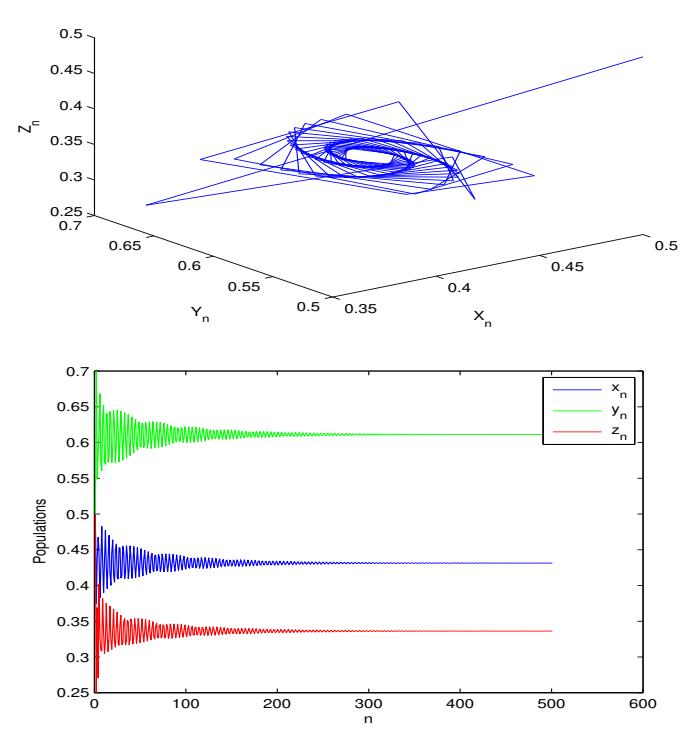
Figure 1: Phase portrait and time series plots of System (3) with parameter values r=4.5, d=1, c=2, w=1, v=1, s=0.1 and initial point (0.5, 0.5, 0.5).
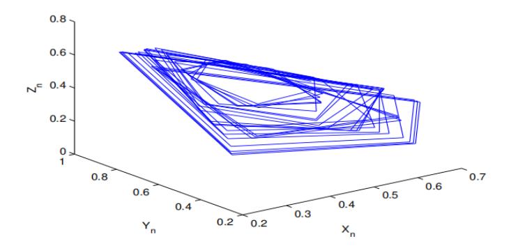
Figure 2: Phase portrait of System (3) with parameter values r=4.5, d=0.3, c=2, w=1, v=1, s=0.1 and initial point (0.5, 0.5, 0.5).
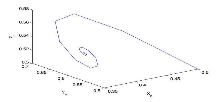
Figure 3: Phase portrait of the controlled System (14) with parameter values \(r=4.5, d=0.3, c=2, w=1, v=1, s=0.1, \rho=0.5\) and initial point (0.5, 0.5, 0.5).
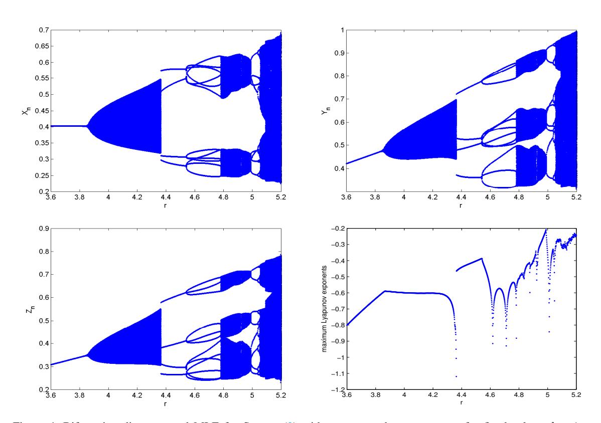
Figure 4: Bifurcation diagrams and MLE for System (3) with respect to the parameter r for fixed values d=1, c=2, w=1, v=1, s=0.1 and initial point (0.5, 0.5, 0.5). As MLE is negative, the behaviour of System (3) is non-chaotic.
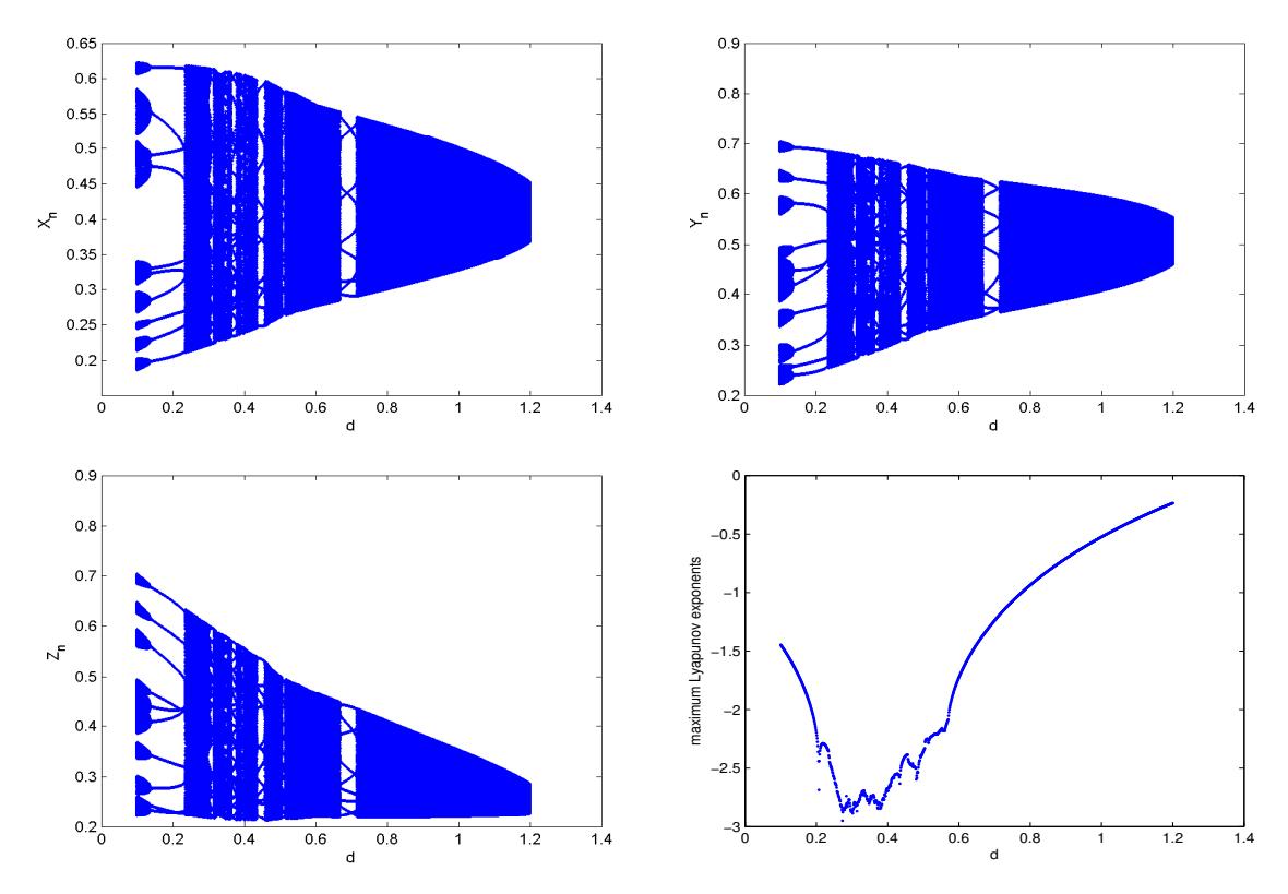
Figure 5: Bifurcation diagrams and MLE for System (3) with respect to the parameter d for fixed values r = 4, c = 2.2, w = 1, v = 1, s = 0.1 and initial point (0.5, 0.5, 0.5). As MLE is negative, the behaviour of System (3) is nonchaotic.
.
6. DISCUSSION
This paper explored the dynamics of a discrete-time model of two genetically distinguished predator population and one prey population. The stability of boundary, interior fixed point and Neimark-Sacker bifurcation are examined. As the trivial fixed point always exist and is locally stable when the parameters r, s and d remain below one. This type of condition should be avoided as it indicates that all the populations go to extinction. When r > 1, the prey only fixed point can exist which may be locally stable under the restriction of the system parameters. In that case, all the populations cannot go to extinction together. The basic results of the model have been studied through phase portrait, bifurcation diagrams and maximum Lyapunov exponents. The proposed model admits more rich characteristics which are not observed in continuous systems. In [4], the authors defined a parameter θ that governs the dynamics of the continuous system. When θ ≥ 1, the predators disappear from the environment and only the prey survive at the environment's carrying capacity. When θ < 1, the two species coexist at steady state. They also remarked that no Hopf bifurcation can arise around the coexistence equilibrium point. In our System (3), we observed Neimark-Sacker bifurcation around the interior fixed point by varying the parameters r and d. We also found chaotic behaviour under certain choice of the system parameters. From our study, it is clear that the intrinsic growth rate of prey species and the mortality rate of predator species z have strong stability effect. We observe that the system becomes stable from chaotic dynamics if we increase the value of d.
Sometimes bifurcation and chaotic behaviour are in fact unwanted circumstances in discrete dynamical systems, because the system cannot persist as long as chaos is occurring. So chaos control becomes a vital issue. To control chaos, we have used the hybrid control method so that the stability of the system can be regained. To our understanding, the dynamical study of discrete ecogenetic model considering predator-prey system has not done yet. Global stability analysis remains for future work.
ACKNOWLEDGEMENT
The author is grateful to the anonymous reviewers for their helpful comments for improving the paper.