

1. Introduction
Trigona sp. is a stingless bee species with a very small size that can produce high-quality commodities such as bee pollen, propolis, and honey [10], [6] that useful in the health sector and for direct consumption. Trigona is commonly found in tropical and subtropical areas such as the United States, Africa, Australia, and Southeast Asia [17], [16]. This bee makes nests on tree branches, bamboo trunks, between rocks, even on the ground [7], [13]. Like other bees in general, this species live by forming colonies consisting of 300 to 80,000 bees and includes 3 castes, i.e. queen bees, worker bees, and male bees (drones) [20], [8].
The queen bee is the largest in the colony [2], its size about 3 times the size of a worker bee, and is in charge of leading the colony and laying most eggs throughout its life with the ability to lay between 1,000-2,000 eggs per day. Queen bees can live for 3-5 years. In every egg-laying period, there will be young queen bee (virgin queen/gynes) eggs that hatch in small numbers [5], then there will be competition between the queen and the gynes to determine who will lead the colony.
Male bees (drones) are classified into two types, haploid and diploid. Haploid male bees come from the eggs of worker bees that have been through the process of parthenogenesis and eggs of the queen bee those are not successfully fertilized by haploid male bees [5], and most haploid bees come from the eggs of the queen bee [9]. Meanwhile, diploid male bees come from the eggs of the queen bee those are successfully
*Corresponding Author
Received November \(14^{th}\), 2022, Revised December \(5^{th}\), 2022, Accepted for publication December \(31^{st}\), 2022. Copyright ©2022 Published by Indonesian Biomathematical Society, e-ISSN: 2549-2896, DOI:10.5614/cbms.2022.5.2.4
fertilized by haploid male bees and have weak characteristics due to their genetic burden [9]. Haploid male bees are in charge of mating with the queen bee and will die immediately after mating with the queen. Most of the diploid male bees will be killed or removed from the hive by worker bees when the season is bad or food supplies run low because they are considered pests [1].
Worker bees are all females whose reproductive organs do not function properly [6], [19]. This type comes from the eggs of a queen bee which are fertilized by an adult haploid male bee. Workers can also produce eggs that will become a haploid male bee [19], [12]. However, the queen bee will still affect the quantity and quality of eggs produced by workers [12]. Worker bees have a really important task in the colony, workers are guarding the colony (armed with resin and bites), looking for bee pollen and nectar (which is done by scattering) [4], taking care of the hive (forming propolis poles, making new honey pots, maintaining the temperature of the hive, reducing honey moisture content, removing the remaining egg shells), and feeding the larvae. The life span of worker bees is about 2 months, and they have a risk of death from being attacked by predators while looking for bee pollen and nectar. [1].
The mating period of the queen bee lasts for 3-7 days, and a queen bee will choose around 7-12 haploid male bees to mate with [1]. The worker bee will then make an egg sac and produce trophic eggs which are consumed by the queen bee, and fill egg sacs with royal jelly as food. The queen bee lays eggs in the egg sac after confirming the availability of feed in the bag [12]. The proportion of male and female eggs is 61:67, and the diploid male proportion of about 50%. The incubation period of egg, larval, and pupal stages was described by Salmah et. al. [15]. Estimated age (in days) for each stage i.e. 0-4.2 for the egg stage, 4.2-14.6 for the larval stage, and 14.6-46.5 for the pupal stage.
Several studies on honey bees have been conducted before, such as [14] which explains that the growth of bee colonies is highly dependent on the availability of food and social inhibition, their model is implemented as a series of difference equations operating at discrete time steps to model changes in bee population day by day and base the rate equations on the analytic models of Khoury et al.[11], and go further by simulating colony growth across three years to capture seasonal and annual growth cycles. Russel suggests that colonies may be especially sensitive to compromised forage situations, shifting seasons, or agents that reduce the survival of both nurse and forager bees. Another research conducted by [3] which models the effect of pollen on honeybee colony dynamics explains that pollen and nectar are foods that are needed by the colony, The model is implemented as a series of difference equations operating at discrete time steps to model changes in bee population day by day. Other research on modeling is also presented in [18] which models honeybee population dynamics by analyzing the increase in larval mortality and the effect of food scarcity so that it disrupts honeybee colonies, their transient model based on differential equations accounts for the effects of pheromones in slowing the maturation of hive bees to foraging bees, the increased mortality of larvae in the absence of sufficient hive bees, and the effects of food scarcity. However, there is still no information available on the modeling of the Dynamic Analysis of Stingless Bee (Trigona sp.). In this paper, we construct a Trigona bee colony model in two different cases, then we examine the positivity of each compartment of the equilibrium point, and we analyze its stability in several cases. To provide clearer illustrations, we present numerical simulations in the form of a simulation graph for each discussion.
2. MATHEMATICAL MODELING
To formulate the mathematical model, we use several assumptions such as there is only one Queen Bee in the colony, the growth rate of eggs turns into larvae is the same in each bee compartment and its period is uniformly distributed, the age of haploid male bee is 30 days, and the age of diploid male bee is 20 days. Besides that, Worker Bees produced 20 eggs/day, kill 1 diploid male bee/day, and there are no predators so Worker Bees only experience natural death or death due to work exhaustion. We will use 9 compartments such as eggs (Ew, Em, and Ed), larvae (Lw, Lm, and Ld), and adult bee compartments (Tw, Tm, and Td) representing worker, haploid male, and diploid male, respectively. We then construct a differential equation model by considering all the factors involved in each compartment and its interactions, and then normalization is carried out based on the number of eggs in the model.
In the egg compartments, the number of eggs will continue to increase from the queen's egg yield according to their respective proportions. In addition, Em will increase from the egg yield Tw by ϕ. After that, all eggs will develop into larvae for 6 days so that all larval compartments will increase in egg development results. All larvae will be fed by Tw so Tw will die if they don't get enough food from Tw. All larvae will develop into adult bees for 42 days. Adult Bees will experience natural death and death due to other factors such as
\(T_w\) will experience death due to exhaustion, \(T_m\) will experience death due to mating with the queen, while \(T_d\) will experience death due to it being killed by \(T_w\) because it is considered a pest.
\[\frac{dE_w}{dt} = \alpha pr - \alpha E_w, \frac{dE_m}{dt} = \alpha (1 - p) + \phi T_w - \alpha E_m, \frac{dE_d}{dt} = \alpha (1 - r)p - \alpha E_d, \frac{dL_w}{dt} = \alpha E_w \left(1 - \frac{\sigma(L_w + L_m + L_d)}{e + T_w}\right) - \gamma L_w, \frac{dL_m}{dt} = \alpha E_m \left(1 - \frac{\sigma(L_w + L_m + L_d)}{e + T_w}\right) - \gamma L_m, \frac{dL_d}{dt} = \alpha E_d \left(1 - \frac{\sigma(L_w + L_m + L_d)}{e + T_w}\right) - \gamma L_d, \frac{dT_w}{dt} = \gamma L_w - \mu_w T_w - \frac{\eta(L_w + L_m + L_d)T_w}{e + T_w}, \frac{dT_m}{dt} = \gamma L_m - \mu_m T_m - \frac{\beta T_m}{c + T_m}, \frac{dT_d}{dt} = \gamma L_d - \mu_d T_d - \frac{\delta T_w T_d}{d + T_d}.\] (1)
We have 15 parameters in Model (1), those are p (success fertilization probability), r (eggs proportion of \(L_w\)), e (feeding frequency of larva), e (mating frequency of \(T_m\) and queen bee), d (The frequency of \(T_d\) killed by \(T_w\)), \(\alpha\) (1/egg period), \(\beta\) (\(T_m\) number needed by the queen bee), \(\gamma\) (1/larval period), \(\delta\) (the number of \(T_d\) killed by \(T_w\)), \(\eta\) (\(T_w\) fatigue level), \(\mu_w\) (1/age \(T_w\)), \(\mu_m\) (1/age \(T_m\)), \(\mu_d\) (1/age \(T_d\)), \(\phi\) (eggs production of \(T_w\) per unit time), and \(\sigma\) (larval death because not being fed by \(T_w\)). In Model (1), the decreasing rate of \(T_m\) follows Holling type II functional response because \(T_m\) will die after mating with the queen bee, so that when \(T_m\) goes to infinity then the number of \(T_m\) that will mate the queen is limited to a number of \(\frac{\beta}{\eta}\). It is also applied to the \(T_d\) compartment, where \(T_w\) will kill \(T_d\) because \(T_d\) is considered as pest that does not have a significant role in the colony. The Holling type II functional response aims to limit the number of \(T_d\) killed by \(T_w\) by \(\frac{\delta}{\zeta}\) for \(T_d\) close to infinity. The function \(\frac{\sigma(L_w + L_m + L_d)}{1 + eT_w}\) in \(4^{\text{th}}\) to \(6^{\text{th}}\) Model (1), shows the effect of \(T_w\) on feeding the larvae. When \(T_w\) goes to infinity, then the function will go to 0 which can be interpreted as the larvae getting enough food. From Model (1), we analyze the existence of each compartment of the coexistence point and its stability.
3. RESULT AND DISCUSSION
In this section, we have three discussions, i.e. the coexistence of the population that can be seen from its equilibrium point, the stability of the equilibrium point which can be seen from the eigenvalue that is obtained from Jacobian matrix, and the numerical simulations in the form of graphics. In each discussion, we classify the matters into two cases: special case (\(\sigma=\eta=0\)) where there is sufficient food for the larvae and no worker bee's death caused by exhaustion, and general case (\(\sigma\neq0\) and \(\eta\neq0\)) where there is insufficient food for the larvae and worker bee's death caused by exhaustion. It is divided into two parts because \(\sigma\) and \(\eta\) influence each other.
3.1. Equilibrium Point and Its Stability Analysis
1) Special Case: \(\mathbf{E_1}=(E_{w_1},E_{m_1},E_{d_1},L_{w_1},L_{m_1},L_{d_1},T_{w_1},T_{m_1},T_{d_1})\) is the equilibrium point of Model (1) for special case with \(E_{w_1}=pr, E_{m_1}=\frac{p\phi r+(1-p)\mu_w}{\mu_w}, E_{d_1}=(1-r)p, L_{w_1}=\frac{\alpha pr}{\gamma}, L_{m_1}=\frac{\alpha(p\phi r+(1-p)\mu_w)}{\gamma\mu_w}, L_{d_1}=\frac{\alpha pr}{\gamma}\), and \(T_{w_1}=\frac{\alpha pr}{\mu_w}\). While \(T_{m_1}\) and \(T_{d_1}\) are obtained in quadratic form and respectively can be seen in Equation (2) and (3).
\[\mu_m \mu_w T_{m_1}^2 + (-\alpha p \phi r - \alpha \mu_w (1 - p) + c \mu_m \mu_w + \beta \mu_w) T_{m_1} - \alpha c (p \phi r + \mu_w (1 - p)) = 0, \tag{2}\]
\[\mu_d \mu_w T_{d_1}^2 + (\alpha \delta pr - \alpha p \mu_w (1 - r) + d\mu_d \mu_w) T_{d_1} - (1 - r) \alpha p d\mu_w = 0.\] (3)
Both \(T_{m_1}\) and \(T_{d_1}\) have positive second-order coefficient and negative constant, which guarantee that \(T_{m_1}\) and \(T_{d_1}\) have positive real root. Because each compartment has one positive value in this special case, then the existence of equilibrium point \(\mathbf{E}_1\) is guaranteed.
By doing linearization around the equilibrium point, we obtained the Jacobian matrix for \(E_1\) as in Equation (4).
\[\text{[rumus tidak dapat ditampilkan dengan baik — lihat PDF asli]}\]
with \(\mathcal{J}=\frac{\beta T_{m_1}-\beta(c+T_{m_1})}{(c+T_{m_1})^2}\) and \(\mathcal{K}=\frac{\delta T_{w_1}T_{d_1}-\delta T_{w_1}(d+T_{d_1})}{(d+T_{d_1})^2}\). From Equation (4), we get nine negative eigenvalues in Equation (5) which shows that \(E_1\) is stable for the special case.
\[\lambda_{1} = \begin{bmatrix} -\alpha & -\alpha & -\alpha & -\gamma & -\gamma & -\gamma & -\mu & -\frac{\mu_{m}(T_{m_{1}}+c)^{2}+\beta c}{(T_{m_{1}}+c)^{2}} & -\frac{\mu_{d}\mu_{w}(T_{d_{1}}+d)^{2}+\alpha d\delta pr}{\mu_{w}(T_{d_{1}}+d)^{2}} \end{bmatrix}.\] (5)
2) General Case: \(\mathbf{E_2} = (E_{w_2}, E_{m_2}, E_{d_2}, L_{w_2}, L_{m_2}, L_{d_2}, T_{w_2}, T_{m_2}, T_{d_2})\) is the equilibrium point of model (1) for general case with \(L_{w_2} = \frac{\alpha p r(\sigma \mu_w + \eta) T_{w_2}}{\gamma(\alpha \sigma p r + \eta T_{w_2})}\), \(L_{m_2} = \frac{(\sigma \mu_w + \eta)(\phi T_{w_2} + \alpha(1-p))T_{w_2}}{\gamma(\alpha \sigma p r + \eta T_{w_2})}\), \(E_{w_2} = pr\), \(E_{m_2} = \frac{\phi T_{w_2} + \alpha(1-p)}{\alpha}\), and \(E_{d_2} = (1-r)p\). While \(L_{d_2}\), \(T_{w_2}\), \(T_{m_2}\), and \(T_{d_2}\) are obtained in quadratic form and can be seen in Equation (6), (7), (8), and (9), respectively.
\[-\frac{(\phi(\sigma\mu_w + \eta) + \gamma\mu_w)T_{w_2}^2 + (\alpha pr(\sigma\mu_w + \eta - \gamma) + e\gamma\mu_w + \alpha(\sigma\mu_w + \eta)(1-p))T_{w_2} - \alpha e\gamma pr}{\gamma(\alpha pr\sigma + \eta T_{w_2})} = 0, \quad (6)\]
\[(\phi(\sigma\mu_w + \eta) + \gamma\mu_w)T_{w_2}^2 - (\alpha(\gamma pr - \sigma\mu_w - \eta) - e\gamma\mu_w)T_{w_2} - \alpha e\gamma pr = 0,\] (7)
\[\mu_{m}(\alpha p r \sigma + T_{w_{2}} \eta) T_{m_{2}}^{2} - (\phi(\sigma \mu_{w} + \eta) T_{w_{2}}^{2} + (\alpha(\sigma \mu_{w} + \eta)(1 - p) - \eta(c\mu_{w} + \beta)) T_{w_{2}} - \alpha p r \sigma(c\mu_{m} + \beta)) T_{m_{2}} - T_{w_{2}}(\sigma \mu_{w} + \eta)(T_{w_{2}} \phi + \alpha(1 - p))c = 0,\] (8)
\[\underbrace{\frac{\mu_d(\alpha pr\sigma + T_{w_2}\eta)T_{d_2}^2 + ((\mu_w(\phi\sigma + \gamma) + \eta(\delta + \phi))T_{w_2}^2 + (\alpha pr\sigma(\delta + \mu_w) + \alpha(\eta + \sigma\mu_w)(1 - p) + \alpha pr(\eta - \gamma) + d\eta\mu_d + e\gamma\mu_w)T_{w_2} + \alpha pr(d\sigma\mu_d - e\gamma))T_{d_2} + d((\phi(\sigma\mu_w + \eta) + \gamma\mu_w)T_{w_2}^2 + (\alpha pr(\sigma\mu_w + \eta - \gamma) + \alpha(\sigma\mu_w + \eta)(1 - p) + e\gamma\mu_w)T_{w_2} - \alpha e\gamma pr)}{\cosh t}} = 0.\]
From Equation (7) and (8), we can see that \(T_{w_2}\) and \(T_{m_2}\) have positive second-order coefficient and negative constant respectively, which guarantee that \(T_{m_2}\) and \(T_{d_2}\) have positive real root. While in Equation (9), we can see that the coefficient of \(T_{d_2}^2\) is positive, but we need a negative constant from Equation (9) to guarantee the existence of \(T_{d_2}\).
Suppose that A is the simplification of the constant of Equation (9). Because d > 0, we can write it as
\[\mathcal{A} = (\phi(\sigma\mu_w + \eta) + \gamma\mu_w)T_{w_2}^2 + (\alpha pr(\sigma\mu_w + \eta - \gamma) + \alpha(\sigma\mu_w + \eta)(1 - p) + e\gamma\mu_w)T_{w_2} - \alpha e\gamma pr. \quad (10)\]
Suppose that \(T_{w_{2,1}}\) and \(T_{w_{2,2}}\) are the roots of Equation (10). Since Equation (10) is a quadratic equation with a graph that opens up and has a positive discriminant, it is obtained that the Equation (10) will be negative when \(T_{w_{2,1}} < T_{w_2} < T_{w_{2,2}}\), so the constant of the Equation (9) will be negative. Thus, there is a positive \(T_{d_2}\) when \(T_{w_{2,1}} < T_{w_2} < T_{w_{2,2}}\). Note that Equation (10) is the opposite of the numerator of Equation (6), so \(L_{d_2}\) will be positive as \(T_{w_{2,1}} < T_{w_2} < T_{w_{2,2}}\). Because each compartment has one positive value in this general case, then the coexistence of equilibrium point \(\mathbf{E_2}\) is guaranteed.
Using the same method as the special case, we can obtain the eigenvalues in the general case using the Jacobian matrix from the equilibrium point \(E_2\) contained in Equation (11).
\[\text{[rumus tidak dapat ditampilkan dengan baik — lihat PDF asli]}\]
with \(\mathcal{B}=\alpha\left(1-\frac{\sigma(L_{w_2}+L_{m_2}+L_{d_2})}{e+T_{w_2}}\right)\), \(\mathcal{C}=-\frac{\alpha\sigma}{e+T_{w_2}}\), \(\mathcal{D}=\frac{\eta T_{w_2}}{e+T_{w_2}}\), \(\mathcal{E}=\frac{\alpha\sigma(L_{w_2}+L_{m_2}+L_{d_2})}{(e+T_{w_2})^2}\), \(\mathcal{F}=\frac{\eta(L_{w_2}+L_{m_2}+L_{d_2})}{e+T_{w_2}}\), \(\mathcal{G}=\frac{\beta}{c+T_{m_2}}\left(\frac{T_{m_2}}{c+T_{m_2}}-1\right)-\mu_m\), and \(\mathcal{H}=\frac{\delta T_{w_2}}{d+T_{d_2}}\left(\frac{T_{d_2}}{d+T_{d_2}}-1\right)-\mu_d\). Based on the Jacobian matrix of equilibrium point in model (1), we obtain five negative eigenvalues analytically in Equation (12)
\[\lambda_2 = \begin{bmatrix} -\alpha & -\alpha & -\gamma & -\frac{\mu_m (T_{m_2} + c)^2 + \beta c}{(T_{m_2} + c)^2} & -\frac{\mu_d (T_{d_2} + d)^2 + T_{w_2} d\delta}{(T_{d_2} + d)^2} \end{bmatrix}.\] (12)
We obtain the remaining eigenvalues from the characteristic equation in Equation (13)
\[A_4\lambda_2^4 + A_3\lambda_2^3 + A_2\lambda_2^2 + A_1\lambda_2 + A_0 = 0, (13)\]
with with \[A_4 = (\alpha pr\sigma + \eta T_{w_2})(e + T_{w_2}),\] \[A_3 = \eta(\phi\sigma + \alpha + 2\gamma + \mu_w)T_{w_2}^2 + ((\alpha\sigma + e(2\gamma + \alpha))\eta + \alpha p\phi r\sigma^2 + pr\alpha(2\gamma + \mu_w + \alpha)\sigma)T_{w_2} + \alpha^2 pr\sigma^2 + \alpha epr(2\gamma + \mu_w + \alpha)\sigma + \alpha e\eta pr,\] \[A_2 = (\phi(\gamma + \alpha)\sigma + 2\alpha\gamma + \alpha\mu_w + \gamma^2 + 2\gamma\mu_w)\eta T_{w_2}^2 + ((\alpha(p\phi r + \alpha + \gamma)\sigma + \gamma e(\gamma + 2\alpha))\eta + \alpha p\phi r(\gamma + \mu_w + \alpha)\sigma^2 + pr\alpha(2\alpha\gamma + \alpha\mu_w + \gamma^2 + 3\gamma\mu_w)\sigma)T_{w_2} + (\alpha^2 pr\sigma + \alpha epr(2\gamma + \alpha))\eta\alpha^2 pr(\gamma + \mu_w + \alpha)\sigma^2 + pr\alpha(-\alpha\gamma pr + 2\alpha e\gamma + \alpha e\mu_w + e\gamma^2 + 2e\gamma\mu_w)\sigma,\] \[A_1 = (\alpha\phi\eta^2 + (\alpha\phi(\gamma + \mu_w)\sigma + \gamma(\alpha\gamma + 2\alpha\mu_w + \gamma\mu_w))\eta)T_{w_2}^2 + ((\alpha(\alpha p\phi r + \gamma p\phi r + \alpha\gamma)\sigma + \gamma^2 \alpha e)\eta + \alpha p\phi r(\alpha\gamma + \alpha\mu_w + \gamma\mu_w)\sigma^2 + \gamma\alpha pr(\alpha\gamma + 3\alpha\mu_w + 2\gamma\mu_w)\sigma)T_{w_2} + (\alpha^2 pr(\gamma + \alpha)\sigma + \gamma\alpha epr(\gamma + 2\alpha))\eta + \alpha^2 pr(\alpha\gamma + \alpha\mu_w + \gamma\mu_w)\sigma^2 + \gamma\alpha pr(\alpha(2e\mu_w - \alpha pr - \gamma pr + e\gamma) + e\gamma\mu_w)\sigma,\] \[A_0 = (\alpha\gamma\phi\eta^2 + (\alpha\gamma\phi\sigma\mu_w + \alpha\gamma^2\mu_w)\eta)T_{w_2}^2 + 2\alpha^2\gamma(p\phi r\sigma^2\mu_w + \eta p\phi r\sigma + \gamma pr\sigma\mu_w)T_{w_2} + (\alpha^3\gamma pr\sigma + \alpha^2 e\gamma^2 pr)\eta + \alpha^3\gamma pr\sigma^2\mu_w + \gamma^2\alpha^2 pr(-\alpha pr + e\mu_w)\sigma.\]
Since Equation (13) is difficult to reduce, so we substitute all parameter values except \(\sigma\) and \(\eta\) to the equation. After obtaining a simpler polynomial function, an analysis are carried out using the criteria Routh-Hurwitz, where if \(B = A_1A_2 - A_0A_3 > 0\) and \(C = BA_3 - A_1^2A_4 > 0\) then we get that all the eigenvalues of Equation (13) have negative values. Based on the substitution of the parameter values and \(T_{w_2} > 0\), we obtained \(B = A_1A_2 - A_0A_3 > 0\). Moreover, \(C = BA_3 - A_1^2A_4\) will have a positive value with sufficient condition \(\eta \leq 0.85\). Then, by using the Routh-Hurwitz criteria [22], all the eigenvalues of Equation (13) will have negative values. Based on the analysis above, we obtain that all the eigenvalues of \(E_2\) from the Equation (11) are negative, or in another word \(E_2\) is a stable equilibrium point.
3.2. Numerical Simulation
For numerical simulation, we used the parameter values as in Table 1.
| Parameter | Description | Value | Unit | Reference | |
|---|---|---|---|---|---|
| p | Success Fertilization Probability | 0.7 | - | [9] | |
| r | Eggs Proportion of \(L_w\) | 0.7 | - | [9] | |
| e | Feeding frequency of Larva | 1 | 1/day | Assumed | |
| c | Mating frequency of \(T_m\) and Queen bee per day | 1 | 1/day | Assumed | |
| d | The frequency of \(T_d\) killed by \(T_w\) | 1 | 1/day | Assumed | |
| \(\alpha\) | 1/egg period | 0.167 | 1/day | [1] | |
| β | \(T_m\) number needed by the Queen Bee | 0.006 | 1/day | [1] | |
| \(\gamma\) | 1/larval period | 0.0238 | 1/day | [1] | |
| δ | The number of \(T_d\) killed by \(T_w\) | 0.0005 | 1/day | Assumed | |
| \(\eta\) | Death of \(T_w\) due to exhaustion per day | 0 & 0.01 | 1/day | Assumed | |
| \(\mu_w\) | \(1/\mathrm{age}\ T_w\) | 0.0167 | 1/day | [1] | |
| \(\mu_m\) | \(1/\text{age }T_m\) | 0.033 | 1/day | Assumed | |
| \(\mu_d\) | 1/age \(T_d\) | 0.05 | 1/day | Assumed | |
| \(\phi\) | Eggs production of \(T_w\) per unit time | 0.01 | 1/day | Assumed | |
| \(\sigma\) | Larval death (not being fed by \(T_m\)) per day | 0 & 0.01 | 1/day | Assumed | |
Table 1: Parameters of Model.
1) System Stability on a Pair of Trigona Compartments Based On \(\sigma\) & \(\eta\): The value for each compartment of the equilibrium points \(\mathbf{E_1}\) and \(\mathbf{E_2}\) can be seen in Table 2.
| Table 2: | Equilibrium | Point | Value | for | \(\mathbf{E_1}\) | and | \(\mathbf{E_2}\). |
|---|
| \(\mathbf{E_1}\) | Value | \(\mathbf{E_2}\) | Value |
|---|---|---|---|
| \[\begin{array}{c} E_{d_1} \\ E_{m_1} \\ E_{w_1} \\ L_{d_1} \\ L_{m_1} \\ L_{w_1} \\ T_{d_1} \\ T_{m_1} \\ T_{w_1} \end{array}\] | 0.21 0.5934131737 0.49 1.473529412 4.163865546 3.438235294 0.6815399558 2.949135524 | \[E_{d_2} \\ E_{m_2} \\ E_{w_2} \\ L_{d_2} \\ L_{m_2} \\ L_{w_2} \\ T_{d_2} \\ T_{m_2} \\ T_{w_2}\] | 0.21 0.4097491047 0.49 1.434108305 2.798212352 3.346252711 0.6752479825 1.978046419 1.832810048 |
Figure 1 is two-dimensional numerical simulation results for \(T_w\), \(T_m\), and \(T_d\) compartments in each given case. The graphs show that each sub-population is coexistent for both special and general cases where each compartment goes to one equilibrium point. Moreover, the size of the population was greater when \(\sigma=\eta=0\) than \(\sigma=\eta=0.01\) which is caused by the effect of larval death due to the insufficient food and \(T_w\) death due to fatigue, which affected the decreased of the population number. But it shows that the sub-population in one colony will continue to exist (coexist) and never experience extinction.
Next, we will show the stability of the adult Trigona population. In the second case, we will use the same initial values for the egg and larval populations.
\[\{E_{w_1}, E_{m_1}, E_{d_1}, L_{w_1}, L_{m_1}, L_{d_1}\} = \{0.49, 0.59, 0.21, 3.43, 4.16, 1.47\},\] \[\{E_{w_2}, E_{m_2}, E_{d_2}, L_{w_2}, L_{m_2}, L_{d_2}\} = \{0.49, 0.40, 0.21, 3.34, 2.79, 1.43\},\]
whereas for \(T_w\), \(T_m\), and \(T_d\) will be varied with
\[\begin{aligned} & \{T_{w_1}, T_{m_1}, T_{d_1}\} = \{(4.86, 4.86, 4.915, 4.92), (2.84, 2.91, 2.84, 2.91), (0.62, 0.64, 0.74, 0.73)\}\,, \\ & \{T_{w_2}, T_{m_2}, T_{d_2}\} = \{(1.8275, 1.84, 1.84, 1.8275), (1.93, 1.93, 1.88, 1.88), (0.67, 0.68, 0.67, 0.68)\}\,. \end{aligned}\]
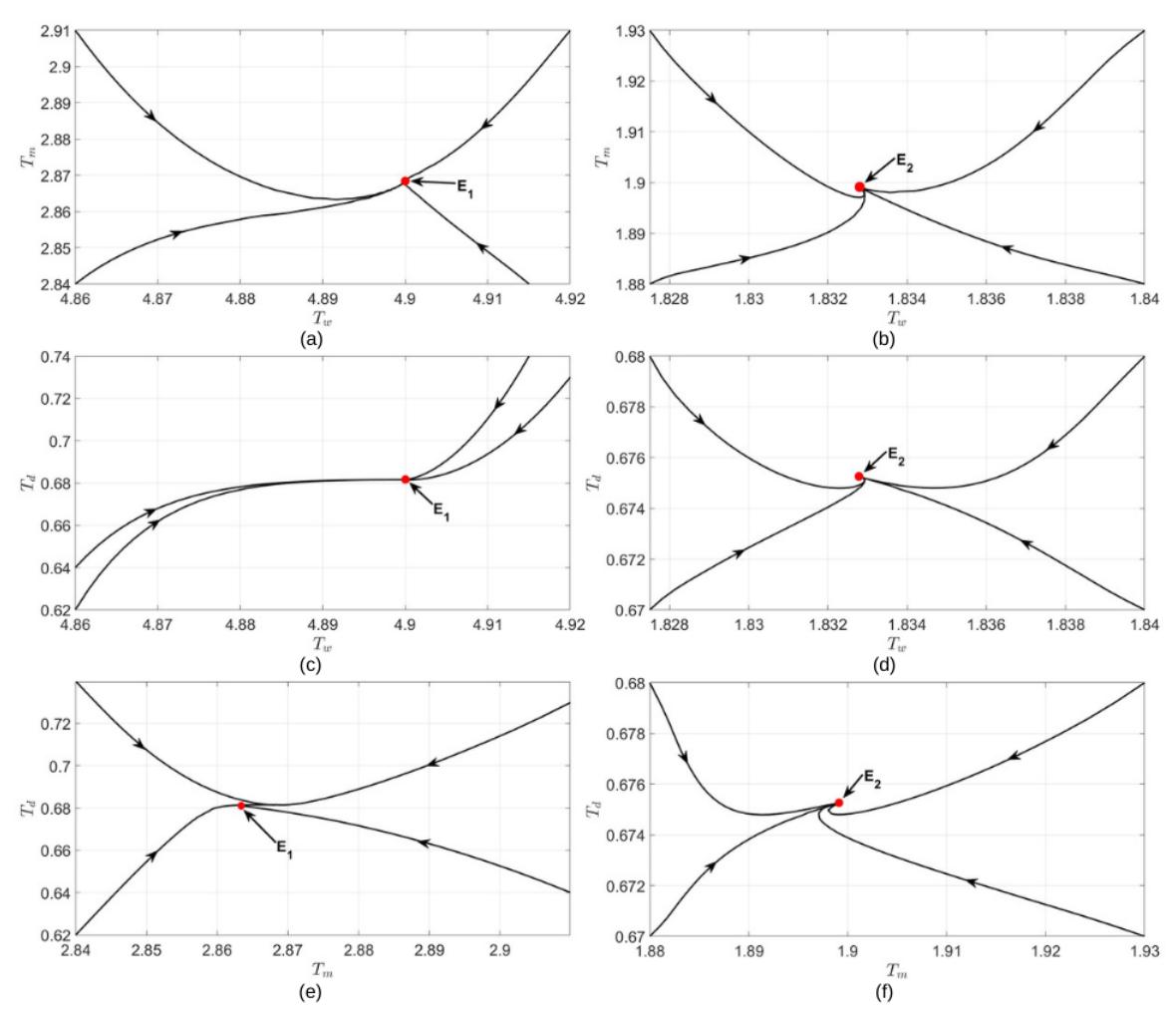
Figure 1: Numerical Simulations of Tw and Tm with (a) σ = η = 0 and (b) σ = η = 0.01, Tw and Td with (c) σ = η = 0 and (d) σ = η = 0.01, Tm and Td with (e) σ = η = 0 and (f) σ = η = 0.01.
2) The Effect of σ and η Parameter's Value: In this section, the sub-population density of each Trigona bee against σ on a certain interval, and a value of η, and vice versa are shown. A graph is presented in each case and shows the effect of σ and η on the Trigona bee sub-populations. Both parameters of σ and η affect the Trigona population. The greater the value of σ or η, the smaller the population density of Tw, Tm, and Td. However, we can see in Figure 2 that the changes of σ value have more significant effects on the population than the ones of η value.
Based on Figure 2, we obtain that if the η value is higher, the number of adult bee populations (Tw, Tm, Td) decreases. It means that if the Tw fatigue level is higher, the Tw population becomes lower so that the larvae do not get enough food. This will also result in a decrease in the number of Tw, Tm, and Td because the number of larvae decreases because they do not get enough food from Tw. Likewise, if the value of σ is higher, the population will decrease. It means that if the mortality of larvae due to insufficient food is higher, there will be fewer larvae that will develop into Tw, Tm, and Td. So the adult bee population will decrease.
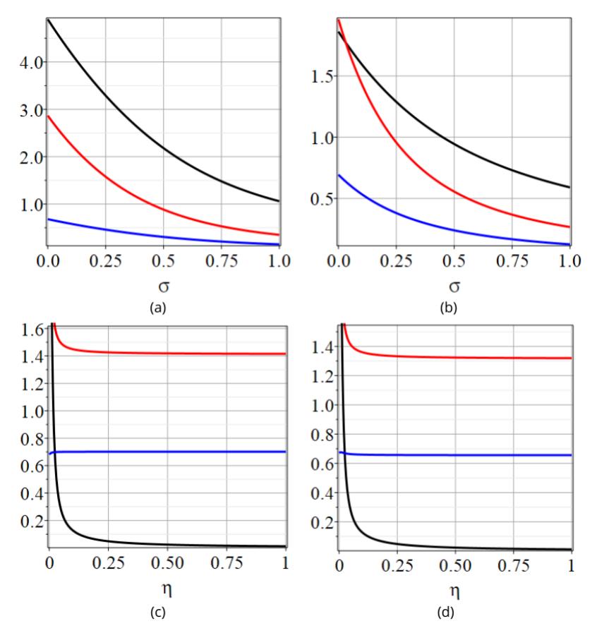
Figure 2: The Effect of σ and η Towards Trigona (a) η = 0 for σ ∈ [0, 1], (b) η = 0.01 for σ ∈ [0, 1], (c) σ = 0 for η ∈ [0, 1], (d) σ = 0.01 for η ∈ [0, 1], with Black, Red, and Blue Curve interpreted by Tw, Tm, and Td Compartment, Respectively.
3) Trigona Bee Population Density Comparison Based on Time: In this section, we present some solution graphics in Figure 3 which show the behavior of the population at the time interval t ∈ [0, 500] for each sub-population in two cases for each graph. In Figure 3, we can see the comparison between solutions in the special and the general case clearly. The entire subpopulations of Trigona bees have a more significant decrease in the general case. This was due to the death of the larvae because their food source from Tw is not enough for all larvae. In addition, the decreased amount of bees in the Trigona population was also caused by the death of Tw caused by exhaustion. This means that in general, there is a significant effect of the σ and η parameters on Trigona sp.'s population growth. It shows that Tw gets the greatest impact in the colony since Tw dies of exhaustion causing the larvae don't get enough food to develop into adults bee. On the other hand, Tm also gets a quite big influence. The decrease of Tw amount will cause Lw's death because their food source from Tw is not enough, and cause the eggs of Tm, that is Em, to decrease. Meanwhile, the population density of Td is not much different in the two cases, because eventhough Tw decreases the number of Ld because their food source from Tw is not enough, the death of Td caused by the Tw kills per time unit is also decreased.
Initial values in Figure 3 are {Tw, Tm, Td} = {4.9, 2.86, 0.68}, and the others are zero because we will only review the differences of Tw, Tm and Td at Special and General case based on time.
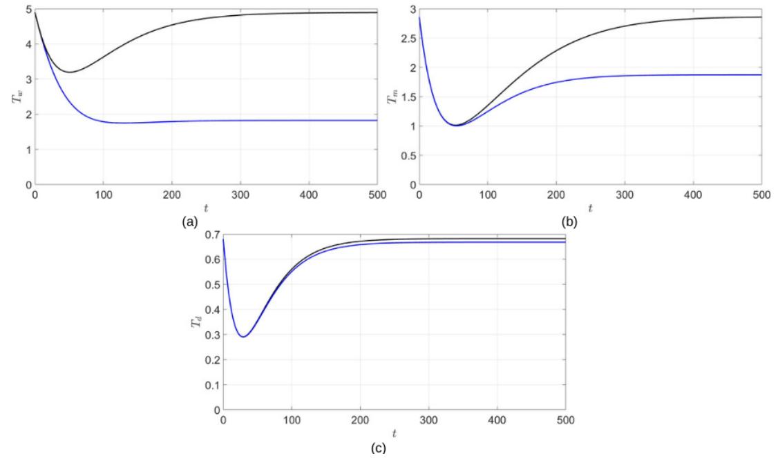
Figure 3: Comparison of Each Trigona's Compartment (a) Tw (b) Tm (c) Td Towards Time t ∈ [0, 500] on Special and General Case in Black and Blue Curve, Respectively.
4. CONCLUSION
From the results and discussion, we conclude that the model of the Trigona bee population has stable coexistence equilibrium points for both special and general cases. It shows that the Trigona bee's colony will remain and continue to grow since there is no change in stability for there is no bifurcation in Model (1) for both cases. Moreover, based on the simulation results, we found that the greater the σ, the lower the number of bees and vice versa. This is also applied to the value of η. From the results, it can be seen that the higher the ability of Tw to feed the larvae, the higher the bee population number. The fatigue level of Tw (η) also affects the number of bees because Tw plays an important role in feeding the larvae. Then, we suggest to the bee farmers to keep maintain food availability by increasing the number of workers in a colony or providing food sources with high contains nectar and propolis at a relatively close distance to reduce the death of worker bees.