

1. INTRODUCTION
Dengue fever is an infectious viral fever that has affected more than 100 nations around the world. Dengue fever (DF) or dengue hemorrhagic fever (DHF), caused by dengue virus (DENV), infects 50 − 100 millions/year, resulting in half a million hospitalizations and 12,500 fatalities [1]. WHO estimates that the number of reported cases of dengue has increased 8 times in the last two decades and 505, 430 and 5.2 million cases were reported in the year 2000 and 2019, respectively [2]. According to a study, 3.9 billion people in 129 different countries, of which 70% are from the Asian continent, are at a higher risk of the infection [3], [4]. The tropical and subtropical regions are considered to be the primary hotspot for dengue spread. However, cases are reported around the globe in the recent years [5].
Female mosquitoes, viz., Aedes aegypti, and partly Aedes albopictus, are the primary carriers of DENV [6]. DENV has four unique variants, namely, DENV-1, 2, 3, and 4. Various symptoms are observed in the patients, caused by these variants. In 2013, the fifth serotype, namely DENV-5, was discovered [7], [8]. Generally, DF is benign in nature. DHF or dengue shock syndrome (DSS) may be observed in some cases [9]. If DHF/DSS is not treated properly and in a timely manner, it can be fatal.
The process of immune response during the infection, caused by DENV, is discussed in-depth to formulate a with-in host model of dengue virus transmission with delayed immune response. Once the virus infects the cells, it starts replicating and emerges out in huge numbers [10], [11], [12]. The newly formed viruses infect
*Corresponding author
Received July 29th, 2022, Revised September 16th, 2022, Accepted for publication October 26th, 2022. Copyright ©2022 Published by Indonesian Biomathematical Society, e-ISSN: 2549-2896, DOI:10.5614/cbms.2022.5.2.1 the other healthy cells again and escalates the transmission. In this situation, the immune system attempts to counter this problem on its own.
Generally, the immune system works in two ways, namely, adaptive and innate immune response. The cell-mediated and the humoral immune response make up the adaptive immune response. The infection is washed out and immunity is provided by both immune responses [13], [14]. It has been found that the humoral immune response plays a more prominent role than the other immune mechanisms during the infection period [15], [16]. During this process, the B-cells attached with the antigen and activate the production of antibodies which in turn neutralize the virus [17]. In most cases, infection takes 4 − 7 days to build up and later the immune response acts [18]. A patient gets infected during the phase of viremia, from which either the patient recovers or continues to be in the leaking phase, which may lead to DHF/DSS [19].
If a person is exposed to DENV first time, then it is called primary infection. Some studies show that longterm immunity against the infection with a serotype is more common [13]. In other words, the immunity against the infection is serotype-specific [20]. Cross-immunity against all variants of DENV is temporary [21]. Furthermore, if someone, who has been already infected by one of the variant of DENV, gets infection by another variant, then it is called as secondary infection. The secondary infection causes serious illness and in some cases, it may be fatal. When the short-term cross-immunity is over, the patients with secondary infection are at a higher risk [22], [23].
The transmission dynamics of DENV in human and mosquito populations have been studied using mathematical modeling by several authors [24], [25]. Halstead et al. [26] presented a mathematical model based on age specific sequential infection rates. May and Nowak [27] proposed mathematical models for virus transmissions inside the body. Several studies have shown the dynamics of the internal transmission of the virus [30], [40], [28], [29], [31]. The concept of delayed immunological response was introduced by Dibrov et al. [32], [33]. Fowler [34] has proposed an approximate solution of a with-in host model with delayed immunity.
Gourley et al.[35] and Li and Shu [36] presented the stability analysis of with-in host models which incorporates the inter-cellular delay. Global stability of an epidemic model with a constant time delay and infectious period is discussed by Huang et al. [37]. Yang et al. [38] illustrated the global dynamics of a within host model describing delayed transmission of both virus to cell and cell to cell. The in-host modeling of humoral immunity with inter-cellular delay is illustrated by Wang and Zou [39]. Tanvi and Ambika [17] considered a model of dengue virus transmission involving humoral immune response incorporating two different time delays to account for the delayed time it takes for B-cells to become plasma cells and generate antibodies. Kanumoori et al. [41] illustrated both immune response combining the time lag in the formulation of antibodies from B cells. Recently, Camargo et al. [42] studied the severity of secondary infection. Sebayang et al. [43] presented a qualitative study of the immune response mediated by antibodies. The detailed biological aspects of the innate immune response are discussed in [44].
Here, a delayed SIVA with-in-host model of dengue virus transmission is presented. A constant delay is thought to be caused by a lag in plasma cell formation from B cells, which causes a delay in the development of antibodies. The suggested model depicts the dynamics of virus transmission with a delayed immune response, as well as the behavior of susceptible, infected, and immune cells.
The model is formulated in Section 2. Section 3 and 4 deal with the analysis of the model and the equilibrium states. The derivation of BRN is presented in Section 5 using NGM method. The detailed stability analysis is discussed in Section 6, using the stability criterion of Lienard - Chipart. Section ´ 7 deals with the bifurcation analysis of the system. The numerical simulation of the model is discussed in Section 8. The sensitivity analysis due to the change in parameters of interest is performed in Section 9. In Section 10, we present the conclusions.
2. MATHEMATICAL FORMULATION
In the development of the mathematical model, the whole cell population N(t) may be divided into four distinct classes S, I, V, and A denoting susceptible cells, infected cells, virus particles and the immune cells, respectively. It is to be noted that the size of these four classes changes with time, i.e., S(t), I(t), V (t), and A(t). The susceptible class denotes the healthy cells which are at a risk of infection and their size is denoted by S(t). The infected class, denoted by I(t), consists of those cells that are already infected by the virus. The virus class describes the free virus particles which are injected in the host and the size of this class is V (t). The A(t) class consists of the immune cells which start the process of immune response. The
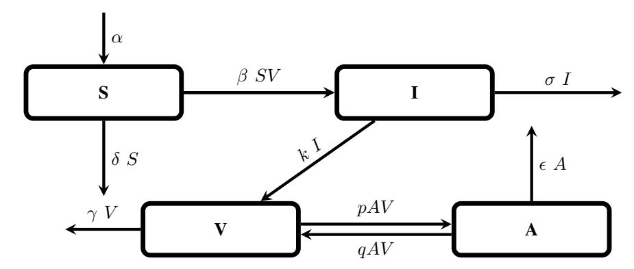
Figure 1: Transmission Diagram.
proposed model represents an approximation to the real life scenario with suitable assumptions such as no other microorganisms attack the body except the dengue virus of one serotype only [30].
To get insight of the dynamics of S, I, V, and A, the following first order coupled system of ODE is proposed:
\[\frac{dS}{dt} = \alpha - \beta \ SV - \delta \ S, \frac{dI}{dt} = \beta \ SV - \sigma \ I, \frac{dV}{dt} = k \ I - \gamma \ V - p \ AV, \frac{dA}{dt} = f \ H(t - \tau) \ V(t - \tau) - q \ AV - \varepsilon \ A.\] (1)
This SIVA model can be elaborated into disjoint compartments as in Figure 1. In Figure 1, every class occupies exactly one compartment and can move from one compartment to another. Each compartment is described as a box and indexed by the class name. The arrows denote the direction of movements of the cells from one class to another. The virus is injected into a healthy individual after the mosquito's bite and attacks the target cells. The target cells are assumed to be the monocytes or macrophages [45]. After coming into contact with V, S become infected and the cells move to the I compartment. The number of infected cells which move from S class to I class, is the product of the densities of S and V, and the associated constant rate is \(\beta\). It is assumed that \(\alpha\) is the rate at which healthy cells enter into the system and \(\delta\) is the rate at which S is washed out of the system. The virus starts replicating inside the infected cells and comes out in large numbers of new viruses at a rate k, which will again infect the susceptible cells. Hence, the number of virus moving from I class to V, is k I, as in Figure 1. \(\sigma\) and \(\gamma\) are assumed to be the decay rates of I and V, respectively. Here, H(t) is the Heaviside step function given as [17],
\[H(t) = \begin{cases} 0, & \text{if } t < 0, \\ 1, & \text{if } t \ge 0. \end{cases}\] (2)
The produced antibodies A attack V and the resulting complex is removed. Thus, a decrease in V and A is observed which is assumed to be the product of V and A [34]. p is considered as the rate at which V is neutralized by A. Antibody-virus complex affects the growth of A at a rate q. It is assumed that the production of plasma cells from B-cells cause a constant delay \(\tau\). The change in A is directly proportional to \(V(t-\tau)\) and the associated rate is f. The Heaviside step function \(H(t-\tau)\) indicates that the generation of plasma cells does not start until a time \(\tau\). \(\varepsilon\) is natural degradation rate of A. Table 1 describes the parameters.
| Parameter Symbol | Parameter Description | Dimensions |
|---|---|---|
| \(\alpha\) | Production rate of S | \(cells \ day^{-1} \ ml^{-1}\) |
| \(\delta\) | Death rate of \(S\) | \(day^{-1}\) |
| \(\beta\) | Rate of infection | \(ml\ virions^{-1}\ day^{-1}\) |
| \(\sigma\) | Death rate of \(I\) | \(day^{-1}\) |
| k | Production rate of \(V\) | \(virions \ day^{-1}\) |
| \(\gamma\) | Elimination rate of V | \(day^{-1}\) |
| p | Neutralizing rate of \(V\) by \(A\) | \(virions\ day^{-1}\) |
| \(\overline{q}\) | Rate at which antibody-virus complex affects the immune cell growth | \(day^{-1}\) |
| \[\frac{\varepsilon}{f}\] | Degradation rate of A Associated rate at which B-cells produce plasma cells | \[\begin{array}{c} day^{-1} \\ day^{-1} \end{array}\] |
Table 1: Parameter Description of (1).
3. ANALYSIS OF THE MODEL
3.1. Positive nature of Solutions
We will prove that the solution of (1) remains positive for all time t if initial conditions are positive. Using (1), we get;
\[\left.\frac{dS}{dt}\right|_{S=0} = \alpha \geq 0, \quad \left.\frac{dI}{dt}\right|_{I=0} = \beta \ S \ V \geq 0, \quad \left.\frac{dV}{dt}\right|_{V=0} = k \ I \geq 0, \quad \text{and} \quad \left.\frac{dA}{dt}\right|_{A=0} = f \ V \geq 0. \quad (3)\]
From (3), it may be noted that the rates are greater than or equal to zero on the planes which is described as S=0, I=0, V=0, and A=0 of the first octant of \(\mathbb{R}^4\). The direction of the vector field of (1) is towards inside on the bounding planes [41]. As a result, if a solution begins within this region then it will remain within this region only, throughout time t. Hence, we conclude that the solutions of (1) continue to be positive if the initial values are always positive for t>0.
3.2. Boundedness of Solutions
To prove the boundedness of the solution, we have N = S + I + V + A. Then, we have the following:
\[\frac{dN}{dt} = \frac{dS}{dt} + \frac{dI}{dt} + \frac{dV}{dt} + \frac{dA}{dt}.\] (4)
Using (1) in (4), we get:
\[\frac{dN}{dt} = \frac{dS}{dt} + \frac{dI}{dt} + \frac{dV}{dt} + \frac{dA}{dt} = (\alpha - \beta SV - \delta S) + (\beta SV - \sigma I) + (kI - \gamma V - pAV) + (fV - qAV - \varepsilon A))\] \[= \alpha + kI + fV - (\delta S + \sigma I + \gamma V + pAV + qAV + \varepsilon A)\] \[< \alpha + kI + fV. \tag{5}\]
As k > f, then rewriting Equation (5) we get:
\[\frac{dN}{dt} \le \alpha + k(I+V). \tag{6}\]
From (5), we have \(\limsup_{t\to\infty} N=\frac{\alpha}{k}\). Therefore, all the solutions of S,I,V, and A are bounded by \(\frac{\alpha}{k}\). To show that the system (1) is bounded in space, we simulate the System at different arbitrarily chosen initial
points, namely, \(P_1 = (400, 50, 100, 50)\), \(P_2 = (200, 20, 80, 200)\), and \(P_3 = (250, 100, 150, 1000)\) and the analysis is discussed in the Section 8.
The region of interest is given as,
\[\Omega = \left\{ (S, I, V, A) \in \mathbb{R}^4 : 0 \le S, I, V, A \le \frac{\alpha}{k} \right\}. \tag{7}\]
4. EQUILIBRIUM STATES OF THE SYSTEM
4.1. Virus-free Equilibrium (VFE) State \(E_0\)
The system (1) exhibits a VFE state \(E_0\) which implies that no virus particles are present in the body. As a result, there is no infected and immune cells. The virus-free equilibrium state \(E_0\) which belong to the boundary of \(\Omega\), is given as \(E_0 = (\frac{\alpha}{\delta}, 0, 0, 0)\).
4.2. Endemic Equilibrium State without immune response \(E_1\)
The system (1) has an ineffective immune response equilibrium state \(E_1\) which incorporates that there is no presence of immune response in the body. Thereby, the ineffective immune response equilibrium state \(E_1\) on the boundary of \(\Omega\), is given as \(E_1 = \left(S_1^*, I_1^*, V_1^*, 0\right)\) where,
\[S_1^* = \frac{\gamma \sigma}{\beta k}, \qquad I_1^* = \frac{\alpha \beta k - \delta \sigma \gamma}{\beta \sigma k}, \quad \text{and} \qquad V_1^* = \frac{\alpha \beta k - \delta \sigma \gamma}{\beta \sigma \gamma}.\] (8)
4.3. Endemic Equilibrium (EE) State \(E_2\)
The EE state \(E_2\) of (1) is given as \(E_2 = (S_2^*, I_2^*, V_2^*, A_2^*)\) where,
\[S_2^* = \frac{\alpha}{(\delta + \beta V_2^*)}, \qquad I_2^* = \frac{\alpha \beta V_2^*}{\sigma (\delta + \beta V_2^*)}, \qquad A_2^* = \frac{f V_2^*}{(\varepsilon + q V_2^*)} \text{ and } V_2^* \text{ is the zero of}\] \[c_0 V_2^{*2} + c_1 V_2^* + c_2 = 0 \quad \text{where,}\] (9)
\[c_0 = \sigma\beta(\gamma q + pf), c_1 = (\beta \gamma \sigma \varepsilon + \delta \sigma \gamma q + \delta \sigma p f - \alpha \beta k q), \text{ and } c_2 = \varepsilon(\delta \sigma \gamma - \alpha \beta k).\] (10)
5. BASIC REPRODUCTION NUMBER (BRN) \((R_0)\)
The number of probable infections caused by one infected cell when remaining cells are not infected is termed as \(R_0\). \(R_0 < 1\) implies that less production of newly infected cells from one infected cell, which results a decrease in the virus population. In the case of \(R_0 > 1\), more newly infected cells are produced which spread the infection rapidly.
To compute \(R_0\), we use the next generation matrix (NGM) method [49]. We consider \(\left(\frac{dI}{dt}, \frac{dV}{dt}\right)\) and follow the same notation as in [49] and compute the vectors \(\mathcal{F}\) and \(\mathcal{U}\) as follows [48]:
\[\mathcal{F} = \begin{pmatrix} \beta & S & V \\ k & I \end{pmatrix} \quad \text{and} \quad \mathcal{U} = \begin{pmatrix} \sigma & I \\ \gamma & V + p & A & V \end{pmatrix}. \tag{11}\]
Now, we have the following Jacobian matrices:
\[F = Jacobian \ of \ \mathcal{F} \ at \ E_0 = \begin{pmatrix} 0 & \frac{\beta \ \alpha}{\delta} \\ k & 0 \end{pmatrix} \quad \text{and} \quad U = Jacobian \ of \ \mathcal{U} \ at \ E_0 = \begin{pmatrix} \sigma & 0 \\ 0 & \gamma \end{pmatrix}. \tag{12}\]
It follows that:
\[F U^{-1} = \begin{bmatrix} 0 & \frac{\alpha \beta}{\delta \gamma} \\ \frac{k}{\sigma} & 0 \end{bmatrix}. \tag{13}\]
The dominant characteristic value of \(F U^{-1}\) is \(R_0\) and is given as,
\[R_0 = \sqrt{\frac{\alpha \beta k}{\delta \sigma \gamma}}. (14)\]
In the following propositions, we write the conditions for existence of the equilibrium states \(E_1\) and \(E_2\) as in Sections 4.2 and 4.3, respectively. It may be noted that these conditions depend on the value of \(R_0\) as in (14).
Proposition 1. Endemic equilibrium state without immune response \(E_1\) exists if \(R_0 > 1\).
Proof: From (8), we have the equilibrium values of S, I, and V. Now, substituting \(R_0\) in the expressions of \(S_1^*\), \(I_1^*\), and \(V_1^*\), we have
\[S_1^* = \frac{\alpha}{\delta R_0^2}, \ I_1^* = \frac{\alpha}{\delta R_0^2} \left( R_0^2 - 1 \right), \ \text{ and } \ V_1^* = \frac{\delta}{\beta} \left( R_0^2 - 1 \right). \tag{15}\]
It is noted that to get the positive equilibrium values of \(S_1^*, I_1^*\), and \(V_1^*\), the following condition must hold,
\[R_0^2 - 1 > 0, (16)\]
(16) can be interpreted as,
\[R_0 > 1. (17)\]
Hence, the proof is completed.
Proposition 2. A unique EE state \(E_2\) exists if \(R_0 > 1\).
Proof: From (9),
\[V_2^* = \frac{-c_1 \pm \sqrt{c_1^2 - 4c_0c_2}}{2c_0}. (18)\]
(18) shows that the product of the two roots is \(\frac{c_2}{c_0}\). If the product of the roots is negative then, it implies that one root is positive and other one is negative.
From (10), the expression for \(c_0\) shows that \(c_0 > 0\). Thus, the product of the roots is negative iff \(c_2 < 0\). Now, rewriting \(c_2\) in terms of \(R_0\), we get,
\[c_2 = \gamma \delta \sigma \varepsilon \left( 1 - R_0^2 \right). \tag{19}\]
Therefore, to obtain a unique EE state \(E_2\), we must have
\[1 - R_0^2 < 0. (20)\]
(20) can be written as,
\[R_0 > 1. (21)\]
It is worth mentioning that the discriminant \(c_1^2 - 4c_0c_2\) in (18) is also positive as \(R_0 > 1\). Thus, we will have a real unique positive EE state \(E_2\) if \(R_0 > 1\). The proof is concluded.
6. STABILITY ANALYSIS
6.1. Stability Analysis of \(E_0\)
Theorem 6.1. The VFE state \(E_0\) is l.a.s iff \(R_0 < 1\) and unstable if \(R_0 \ge 1\).
Proof: To illustrate the stability of VFE state \(E_0\), we linearise (1) about \(E_0\) and get:
\[\frac{dY(t)}{dt} = J_1 Y(t) + J_2 Y(t - \tau) \quad \text{where,}\] (22)
\[\text{[rumus tidak dapat ditampilkan dengan baik — lihat PDF asli]}\] for all \(t > \tau\) and \(Y = (S, I, V, A)^T\).
The characteristic equation of (22) is given as follows:
\[(\lambda + \delta)(\lambda + \varepsilon)\left(\lambda^2 + (\gamma + \sigma)\lambda + \gamma\sigma - \frac{\alpha\beta k}{\delta}\right) = 0.\] (23)
From equation (23), it is observed that the characteristic values are \(-\delta\), \(-\varepsilon\) and the zeros of
\[\lambda^2 + (\gamma + \sigma)\lambda - \gamma \sigma (R_0^2 - 1) = 0, \tag{24}\]
which are given as
\[\lambda_{1,2} = \frac{-(\gamma + \sigma) \pm \sqrt{(\gamma + \sigma)^2 + 4 \gamma \sigma (R_0^2 - 1)}}{2}.\] (25)
Now, we consider the following two cases.
1) Case I, \(R_0 < 1\): From (25), we get:
\[4 \gamma \sigma (R_0^2 - 1) < 0,\]
\[(\gamma + \sigma)^2 + 4 \gamma \sigma (R_0^2 - 1) < (\gamma + \sigma)^2.\]
(26)
Taking square root of both the sides of the inequality (26),
\[\pm\sqrt{(\gamma+\sigma)^2+4\ \gamma\ \sigma\ (R_0^2-1)} < \pm(\gamma+\sigma),\]
\[-(\gamma+\sigma)\pm\sqrt{(\gamma+\sigma)^2+4\ \gamma\ \sigma\ (R_0^2-1)} < -(\gamma+\sigma).\] (27)
This implies that, if \(R_0 < 1\) then the zeros of (24) have negative real values.
2) Case II, \(R_0 > 1\): From (25), we get:
\[4 \gamma \sigma (R_0^2 - 1) > 0.\] (28)
The last term of (24), i.e., \(-\gamma \sigma (R_0^2 - 1)\) is the product of the two zeros and using Equation (28), the product of the two zeros is negative. This implies that if \(R_0 > 1\) then one zero has non-negative real value and the other one has a negative real value.
3) Case III, \(R_0=1\): From (25), we have \(\lambda_1=0\) and \(\lambda_2=-(\gamma+\sigma)\). Thus one root is exactly equal to 0. Thus, if \(R_0=1\) then the \(E_0\) is not stable. Hence, \(E_0\) is l.a.s when \(R_0<1\) and unstable if \(R_0\geq 1\). This completes the proof.
6.2. Stability Analysis of \(E_1\)
We linearise (1) near \(E_1\) and get:
\[\frac{dY(t)}{dt} = L_1 Y(t) + L_2 Y(t - \tau), \tag{29}\]
where
\[\text{[rumus tidak dapat ditampilkan dengan baik — lihat PDF asli]}\] for all \(t > \tau\) and \(Y = (S, I, V, A)^T\). The values of \(S_1^*, I_1^*\), and \(V_1^*\) are given in (8).
The characteristic values of the linearised system (29) are the zeros of,
\[\lambda^4 + a_1 \lambda^3 + a_2 \lambda^2 + a_3 \lambda + a_4 + e^{-\lambda \tau} (a_5 \lambda^2 + a_6 \lambda + a_7) = 0, \tag{31}\]
where
\[\begin{split} a_1 &= \delta + \sigma + \gamma + \varepsilon + \beta V_1^* + q V_1^*, \\ a_2 &= \sigma(\varepsilon + \gamma + q V_1^*) + (\varepsilon + q V_1^*) \gamma - \beta k S_1^* + (\delta + \beta V_1^*) (\varepsilon + \gamma + \sigma + q V_1^*), \\ a_3 &= \gamma \sigma(\varepsilon + q V_1^*) - \beta k S_1^* (\varepsilon + q V_1^*) + (\delta + \beta V_1^*) ((\varepsilon + \gamma + q V_1^*) \sigma \\ &\quad + (\varepsilon + q V_1^*) \gamma - \beta k S_1^*) + \beta^2 k S_1^* V_1^* \\ a_4 &= (\delta + \beta V_1^*) (\gamma \sigma(\varepsilon + q V_1^*) - \beta k S_1^* (\varepsilon + q V_1^*)) + \beta^2 k S_1^* V_1^* (\varepsilon + q V_1^*) \\ a_5 &= p f V_1^*, \quad a_6 &= p f V_1^* (\delta + \beta V_1^*) + p \sigma f V_1^*, \quad \text{and} \quad a_7 &= p \sigma f V_1^* (\delta + \beta V_1^*). \end{split}\]
Now we consider the following two cases:
1) Case I, \(\tau = 0\): If \(\tau = 0\), then (31) becomes;
\[\lambda^4 + D_1 \lambda^3 + D_2 \lambda^2 + D_3 \lambda + D_4 = 0 \quad \text{where,}\] \[D_1 = a_1, \ D_2 = a_2 + a_5, \ D_3 = a_3 + a_6, \ \text{and} \ D_4 = a_4 + a_7.\] (32)
In order to check the nature of the zeros of (32), we construct a Hurwitz matrix H of (32), which is given as:
\[H = \begin{bmatrix} D_1 & D_3 & 0 & 0 \\ 1 & D_2 & D_4 & 0 \\ 0 & D_1 & D_3 & 0 \\ 0 & 1 & D_2 & D_4 \end{bmatrix}. \tag{33}\]
Using the stability criterion of Liénard and Chipart [46], [47], all the zeros of (32) have negative real parts iff \(D_4 > 0\), \(D_2 > 0\); \(\Delta_1 > 0\), \(\Delta_3 > 0\) where, \(\Delta_1 = D_1\) and
\[\Delta_3 = \begin{vmatrix} D_1 & D_3 & 0 \\ 1 & D_2 & D_4 \\ 0 & D_1 & D_3 \end{vmatrix} . \tag{34}\]
Hence, the real part of all the four characteristic values of (32) is negative iff it satisfies the following condition:
\[D_1 D_2 D_3 - D_1^2 D_4 - D_3^2 > 0.\] (35)
The above discussion can be concluded in the following theorem:
Theorem 6.2. The endemic equilibrium state without immune response \(E_1\) of (1) with \(\tau = 0\) is l.a.s iff it satisfies the condition (35) provided that \(D_1, D_2\), and \(D_4\) are greater than 0.
2) Case II, \(\tau > 0\): If \(\tau > 0\), then (31) is a transcendental equation which has infinitely many roots. By Rouché Theorem [50] and continuity in \(\tau\), (31) has a zero with positive real part iff it has purely imaginary root. In other words, all the zeros of (31) will have negative real part if none of them is purely imaginary.
To check that (31) has a purely imaginary zero or not, we put \(\lambda = i \omega\), where, \(\omega \in \mathbb{R}\), in the equation (31). After the substitution, we separate the real and imaginary parts and get:
\[\omega^4 - a_2 \ \omega^2 + a_4 = (a_5 \ \omega^2 - a_7) \cos \omega \tau - a_6 \omega \sin \omega \tau, \tag{36}\]
\[-a_1 \,\omega^3 + a_3 \,\omega = -(a_5 \,\omega^2 - a_7)\sin\omega\tau - a_6\omega\cos\omega\tau. \tag{37}\]
Squaring and adding (36) and (37), we get:
\[(\omega^4 - a_2 \ \omega^2 + a_4)^2 + (a_3 \ \omega - a_1 \ \omega^3)^2 = (a_5 \ \omega^2 - a_7)^2 + a_6^2 \omega^2.\] (38)
Now, we substitute \(\omega^2 = m\) in (38) and get the following:
\[m^4 + R_1 m^3 + R_2 m^2 + R_3 m + R_4 = 0\] where, (39)
\[R_1 = a_1^2 - 2a_2, \ R_2 = a_2^2 + 2a_4 - 2a_1a_3 - a_5^2, \ R_3 = a_3^2 - 2a_2a_4 + 2a_5a_7 - a_6^2, \ \text{and} \ R_4 = a_4^2 - a_7^2.\]
It is observed that (39) will have all the zeros with negative real part iff it satisfies the stability criterion of Liénard and Chipart.
Using the stability criterion of Liénard and Chipart, all the zeros of the equation (39) have negative real parts iff \(R_4 > 0, R_2 > 0; \Delta_1 > 0, \Delta_3 > 0\) where, \(\Delta_1 = R_1\) and
\[\Delta_3 = \begin{vmatrix} R_1 & R_3 & 0 \\ 1 & R_2 & R_4 \\ 0 & R_1 & R_3 \end{vmatrix}. \tag{40}\]
Therefore the zeros of (39) will have negative real part iff \(R_4 > 0\), \(R_2 > 0\); \(\Delta_1 = R_1 > 0\) and it satisfies the following condition:
\[R_1 R_2 R_3 - R_1^2 R_4 - R_3^2 > 0. (41)\]
The following theorem summarises the preceding discussion.
Theorem 6.3. When \(\tau > 0\), the endemic equilibrium state without immune response \(E_1\) of (1) is l.a.s iff it satisfies (41) provided that \(R_1 > 0\), \(R_2 > 0\), and \(R_4 > 0\).
6.3. Stability Analysis of \(E_2\)
We linearize (1) around the point \(E_2\) to investigate the stability of the EE state. After linearizing the system (1), we get:
\[\frac{dY(t)}{dt} = G_1 Y(t) + G_2 Y(t - \tau) \quad \text{where,}\] (42)
\[\text{[rumus tidak dapat ditampilkan dengan baik — lihat PDF asli]}\] for all \(t > \tau\) and \(Y = (S, I, V, A)^T\).
The characteristic values of (42) are the zeros of;
\[\lambda^4 + b_1 \lambda^3 + b_2 \lambda^2 + b_3 \lambda + b_4 + e^{-\lambda \tau} (b_5 \lambda^2 + b_6 \lambda + b_7) = 0 \quad \text{where,}\] (44)
\[\begin{split} b_1 &= \delta + \sigma + \gamma + \varepsilon + \beta V_2^* + q V_2^* + p A_2^*, \\ b_2 &= \sigma(\varepsilon + \gamma + q V_2^* + p A_2^*) + (\varepsilon + q V_1^*)(\gamma + p A_2^*) - \beta k S_2^* + (\delta + \beta V_2^*) \\ &\quad (\varepsilon + \gamma + \sigma + q V_2^* + p A_2^*) - p q A_2^* V_2^*, \\ b_3 &= (\delta + \beta V_2^*) \Big( (p A_2^* + \gamma)(q V_2^* + \varepsilon) - p q A_2^* V_2^* + \sigma(p A_2^* + \gamma + q V_2^* + \varepsilon) \Big) + \beta^2 k S_2^* V_2^* \\ &\quad - \beta k S_2^* (q V_2^* + \varepsilon + \delta + \beta V_2^*) + \sigma \Big( (p A_2^* + \gamma)(q V_2^* + \varepsilon) - p q A_2^* V_2^* \Big), \\ b_4 &= (\delta + \beta V_2^*) \Big( \sigma(p A_2^* + \gamma)(q V_2^* + \varepsilon) - p q \sigma A_2^* V_2^* - \beta k S_2^* (q V_2^* + \varepsilon) \Big) \\ &\quad + \beta^2 k S_2^* V_2^* (q V_2^* + \varepsilon), \\ b_5 &= p f V_2^*, \ b_6 = p f V_2^* (\delta + \sigma + \beta V_2^*), \ \text{and} \ b_7 = p \sigma f V_2^* (\delta + \beta V_2^*). \end{split}\]
Now we consider the following two cases:
1) Case I: \(\tau = 0\): When \(\tau = 0\), the stability analysis of \(E_2\) is similar to the stability analysis of \(E_1\) as described in the Section 6.2.1. Thereby, the characteristic equation (44) becomes as follows:
\[\lambda^4 + M_1 \lambda^3 + M_2 \lambda^2 + M_3 \lambda + M_4 = 0\] where, (45)
\[M_1 = b_1\], \(M_2 = b_2 + b_5\), \(M_3 = b_3 + b_6\), and \(M_4 = b_4 + b_7\).
Using the stability criterion of Liénard and Chipart, all the zeros of (45) have negative real parts iff \(M_4 > 0, M_2 > 0; \Delta_1 > 0, \Delta_3 > 0\) where, \(\Delta_1 = M_1\) and
\[\Delta_3 = \begin{vmatrix} M_1 & M_3 & 0 \\ 1 & M_2 & M_4 \\ 0 & M_1 & M_3 \end{vmatrix}. \tag{46}\]
Hence,the zeros of (45) will have negative real part iff \(M_4 > 0, M_2 > 0; \Delta_1 = M_1 > 0\) and it satisfies the following condition:
\[M_1 M_2 M_3 - M_1^2 M_4 - M_3^2 > 0. (47)\]
We sum up the above discussion in the form of the following theorem:
Theorem 6.4. When \(\tau = 0\), the EE state \(E_2\) of (1) is l.a.s iff it satisfies (47) provided that \(M_1 > 0\), \(M_2 > 0\), and \(M_4 > 0\).
2) Case II: \(\tau > 0\): If \(\tau > 0\), the stability analysis of (44) is similar to Section 6.2.2. We substitute \(\lambda = i \omega\), where, \(\omega \in \mathbb{R}\), in (44) and separate the real and imaginary parts;
\[\omega^4 - b_2 \ \omega^2 + b_4 = (b_5 \ \omega^2 - b_7) \cos \omega \tau - b_6 \omega \sin \omega \tau, \tag{48}\]
\[-b_1 \,\omega^3 + b_3 \,\omega = -(b_5 \,\omega^2 - b_7)\sin\omega\tau - b_6\omega\cos\omega\tau. \tag{49}\]
After squaring and adding (48) and (49), we get:
\[(\omega^4 - b_2 \ \omega^2 + b_4)^2 + (b_3 \ \omega - b_1 \ \omega^3)^2 = (b_5 \ \omega^2 - b_7)^2 + b_6^2 \omega^2.\] (50)
Now, we substitute \(\omega^2 = m\) in (50);
\[m^4 + T_1 m^3 + T_2 m^2 + T_3 m + T_4 = 0\] where, (51)
\[T_1 = b_1^2 - 2b_2\], \(T_2 = b_2^2 + 2b_4 - 2b_1b_3 - b_5^2\), \(T_3 = b_3^2 - 2b_2b_4 + 2b_5b_7 - b_6^2\), and \(T_4 = b_4^2 - b_7^2\). (52)
It may be noted that the zeros of (51) will have negative real part iff it satisfies the stability criterion of Liénard and Chipart, i.e., iff \(T_4>0, T_2>0; \Delta_1>0, \Delta_3>0\) where, \(\Delta_1=T_1\) and
\[\Delta_3 = \begin{vmatrix} T_1 & T_3 & 0 \\ 1 & T_2 & T_4 \\ 0 & T_1 & T_3 \end{vmatrix}. \tag{53}\]
Thereby, the zeros of (51) will have negative real part iff \(T_1 > 0, T_4 > 0\), and \(T_2 > 0\) and satisfies the following condition:
\[T_1 T_2 T_3 - T_1^2 T_4 - T_3^2 > 0. (54)\]
It may be noted that (51) will have at least one positive root if \(T_4 < 0\). In other words, if \(b_4 < b_7\), then (51) will have a positive root. The preceding discussion is outlined as the following theorem:
Theorem 6.5. When \(\tau > 0\), the EE state \(E_2\) of (1) is l.a.s iff it satisfies (54) provided that \(T_1 > 0, T_2 > 0\), and \(T_4 > 0\).
7. BIFURCATION ANALYSIS
Here, \(\tau\) is used as a bifurcation parameter. We consider the polynomial (44), as a function of \(\tau\).
\[z(\lambda) = \lambda^4 + b_1 \lambda^3 + b_2 \lambda^2 + b_3 \lambda + b_4 + e^{-\lambda \tau} (b_5 \lambda^2 + b_6 \lambda + b_7)\] (55)
Let, \(\lambda(\tau) = \eta(\tau) + i\omega(\tau)\) be the characteristics values of (55). It is assumed that a positive root of (51) is \(\omega(\tau_k) = \omega_1\) for some random value of the bifurcation parameter \(\tau_k\). From the equation (48) and (49), we have the following:
\[\omega^4 - b_2 \ \omega^2 + b_4 = (b_5 \ \omega^2 - b_7) \cos \omega \tau - b_6 \omega \sin \omega \tau\] and (56)
\[-b_1 \,\omega^3 + b_3 \,\omega = -(b_5 \,\omega^2 - b_7)\sin\omega\tau - b_6\omega\cos\omega\tau. \tag{57}\]
Assuming \(\omega_1 > 0\), we have the following:
\[\tau_{j} = \frac{1}{\omega_{1}} \arccos \left[ \frac{(b_{5}\omega_{1}^{2} - b_{7})(\omega_{1}^{4} - b_{2}\omega_{1}^{2} + b_{4}) - b_{6}\omega_{1}(b_{3}\omega_{1} - b_{1}\omega_{1}^{3})}{(b_{5}\omega_{1}^{2} - b_{7})^{2} + b_{6}^{2}\omega_{1}^{2}} \right] + 2j\pi, j = 0, 1, 2, \dots\] (58)
It is important to mention that the value of \(\tau\) for which (1) is stable, is given in (58). Differentiating (44) w.r.t \(\tau\), we get:
\[\left(\frac{d\lambda}{d\tau}\right)^{-1} = \frac{4\lambda^3 + 3b_1\lambda^2 + 2b_2\lambda + b_3}{e^{-\lambda\tau} (b_5 \lambda^2 + b_6 \lambda + b_7)} + \frac{2b_5 \lambda + b_6}{\lambda(b_5 \lambda^2 + b_6 \lambda + b_7)} - \frac{\tau}{\lambda}\] (59)
Using (50) in (59),
\[\left[ Re \left( \frac{d\lambda}{d\tau} \right)^{-1} \right]_{\lambda = i\omega_1} = \frac{1}{\omega_1^2} \left( 3\omega_1^8 + T_1\omega_1^6 + T_2\omega_1^4 - T_4 \right) \tag{60}\] where, \(T_1, T_2\), and \(T_4\) are as in (52). From (52), it is easy to say that \(T_1 > 0\) and \(T_2 > 0\). If \(T_4 < 0\) then \(\left[Re\left(\frac{d\lambda}{d\tau}\right)^{-1}\right]_{\lambda=i_{GU}} > 0\). In other words,
\[\left[ Re \left( \frac{d\lambda}{d\tau} \right)^{-1} \right]_{\lambda = i, \nu} > 0 \quad \text{iff} \quad b_4 < b_7.\] (61)
If (61) holds, then \(\frac{dRe\left(\lambda(\tau)\right)}{d\tau} > 0\) and by continuity \(Re(\lambda) > 0\). Hence, the transversality condition for Hopf bifurcation is satisfied [54] and encapsulate the above discussion in the following Theorem:
Theorem 7.1. If \(b_4 < b_7\), then the EE state \(E_2\) is l.a.s when \(\tau < \tau_0\) (using Butler's Lemma [52]) and becomes unstable when \(\tau > \tau_0\).
When \(\tau = \tau_0\), a Hopf bifurcation occurs and the System (1) obtains periodic solutions as \(\tau\) passes through \(\tau_0\) [53].
8. NUMERICAL SIMULATION
We use MATLAB to solve (1) numerically. Table 2 refers to the input data used in the simulation. The initial values of S, I, V, A are given as P = (S, I, V, A) = (200, 50, 100, 50). Using the input data, given in the Table 2, \(R_0 = 2\), the VFE point \(E_0 = (200, 0, 0, 0)\), the endemic equilibrium point without immune response \(E_1 = (50, 15, 150, 0)\) and the EE point is \(E_2 = (79.23, 12.08, 76.21, 1.95)\). Now, we consider three scenarios.
| Parameter Symbol | Parameter Description | Value | Source |
|---|---|---|---|
| α | Production rate of S | 10 | [41] |
| δ | Death rate of S | 0.05 | [17] |
| β | Rate of infection | 0.001 | [17] |
| σ | Death rate of I | 0.5 | [17] |
| k | Production rate of V | 5 | [40] |
| γ | Elimination rate of V | 0.5 | [17] |
| p | Neutralizing rate of V by A | 0.001 | [17] |
| q | Rate at which antibody-virus complex affects the immune cell growth | 0.001 | [17] |
| ε | Degradation rate of A | 0.002 | [51] |
| f | Associated rate at which B-cells produce plasma cells | 0.3 | [41] |
Table 2: Description of the input data.
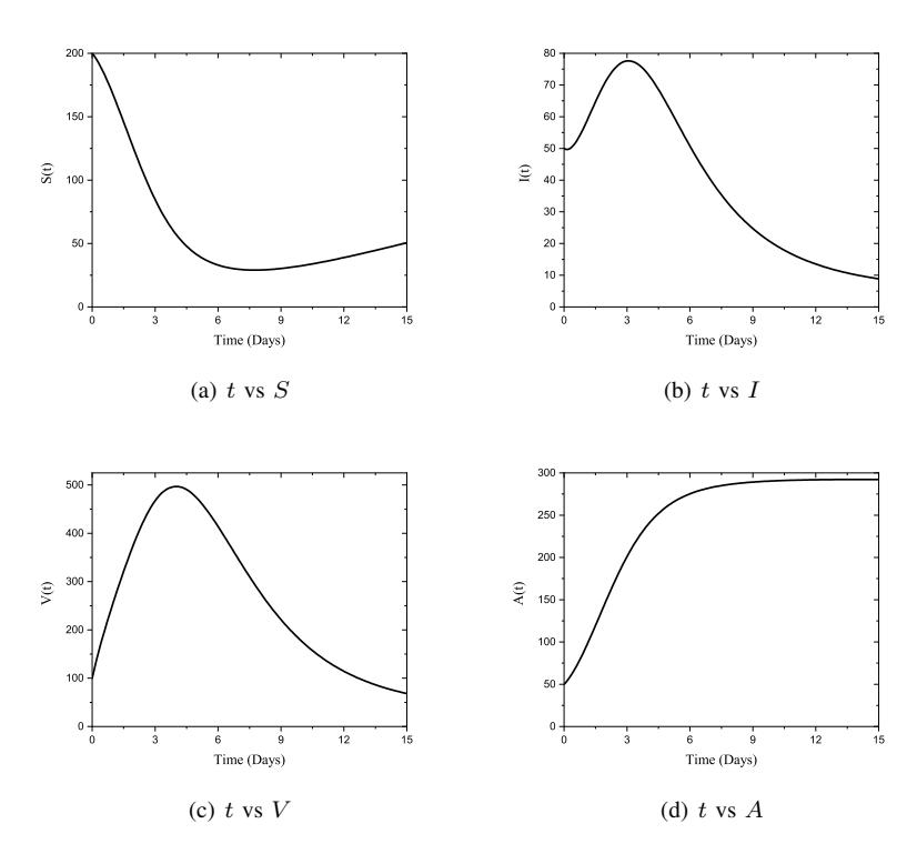
Figure 2: Numerical simulation of S, I, V, and A of (1) when τ = 0.
1) Case I, τ = 0: When τ = 0, for the data provided in Table 2, the maximum number of I is 80.7 which is attained approximately in 3 days as shown in Figure 2(b). From Figure 2(c), we observe that the maximum number of V is 644 and the time it takes to get there is about 5 days.. The dynamics of S and I are also shown in the Figures 2(a) and 2(d), respectively.
It may be noted that for E1, the values of D1, D2, D3, and D4 are 1.35, 0.43, 0.1 and 0.01, respectively. It is also observed that the value of the stability condition given by (35) is 0.03. Hence the endemic equilibrium state without the immune response E1 is l.a.s when τ = 0. For the EE state E2, the values of M1, M2, M3, and M4 are 1.21, 0.1, 0.03 and 0.00001, respectively. The value of the condition of stability for the endemic equilibrium state E2, given in the equation (47), is 0.00212. Thereby, the EE state E2 is l.a.s when τ = 0.
We simulate (1) for randomly chosen initial points P1, P2, and P3, as mentioned earlier. The graphs of the simulation are presented in the Figure 3.
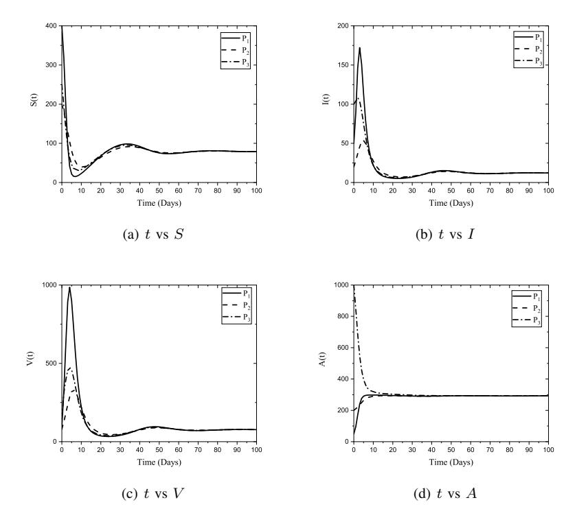
Figure 3: Numerical simulation of S, I, V, and A for different starting points P1, P2, and P3.
- 2) Case II, τ = 0.8: We present the dynamics of S, I, V, and A for τ = 0.8 in Figure 4(a). It may be noted that the maximum number of I is 78.95 which is attained approximately in 3 days. The maximum number of virus particles is 526.1 and the time taken to achieve the maximum number of virus particles is approximately 3.7 days. It is observed that the susceptible cells decrease exponentially and increase again approximately 8 days after the infection. We also observe an exponential growth in the case of immune cells.
- 3) Case III, τ = 5: For τ = 5, the numerical simulation of S, I, V, and A is shown in Figure 4(b). The maximum number of I and V are 79.52 and 613.21, respectively. It may be noted that the time taken to achieve the maximum number of I and V are approximately 3.5 days and 5 days, respectively. The susceptible cells follow the same behavior as described in the case of τ = 0.8. The growth of the immune cells is slow initially but approximately after 6 days the growth of A is exponential.
8.1. Stability Diagram
In this section, we illustrate the stability diagram for both cases τ = 0 and τ > 0 for the equilibrium states E1 and E2. We vary the parameter α from 0 to 30 and k from 0 to 300. Other parameters are fixed as in Table 2. Figure 5 illustrates the stability diagram for the equilibrium state E1. Figure 5(a) shows that when τ = 0, the condition (35) takes positive values as R0 increases. When τ > 0, the condition (41) takes negative values as in Figure 5(b).
Figure 6 refers to the stability diagram for E2. When τ = 0, (47) takes positive values with an increasing value of R0 as shown in Figure 6(a). Figure 6(b) shows the similar behavior for the condition (54).
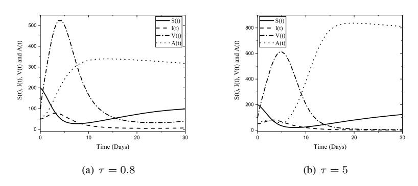
Figure 4: Numerical simulations of S, I, V, and A of (1) when \(\tau > 0\).
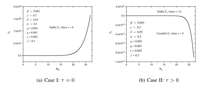
Figure 5: Stability diagram of \(E_1\): left: \(\Delta_3\) as in (35) and right: \(\Delta_3\) as in (41).
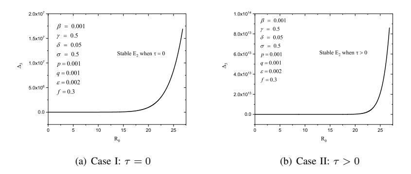
Figure 6: Stability diagram of \(E_2\): left: \(\Delta_3\) as in (47) and right: \(\Delta_3\) as in (54).
8.2. Bifurcation Simulation
Using the value of k=59, f=0.7 and other values as in Table 2, we solve (44) and find that (44) has a pair of purely imaginary root \(\pm 0.65i\) for the critical value \(\tau_0=1.53\). It may be noted that the value
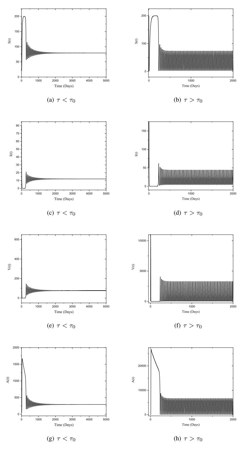
Figure 7: Numerical simulation of S, I, V, and A of (1) when τ < τ0 and τ > τ0.
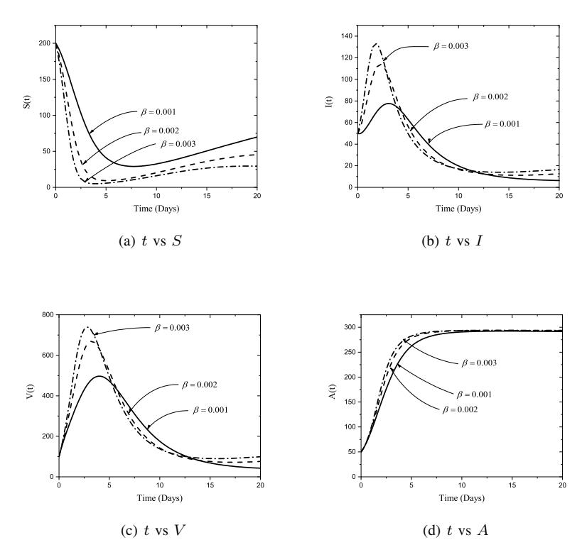
Figure 8: Impact of β on Model (1).
of b4 = 0.063 and b7 = 0.3220. Thus, " Re dλ dτ −1 # λ=iω1 > 0. The numerical simulation of S, I, V, and A for τ < τ0 and τ > τ0 is presented in Figure 7. The initial value of S, I, V, and A is taken as P = (200, 50, 100, 50). We observe that the EE state E2 exhibits a stable behavior when τ < τ0. When τ > τ0, the System obtains a periodic solution or more complex behavior as the Hopf bifurcation occurs.
8.3. Data Sensitivity
The sensitivity analysis is done to see the impact of changes in the data on (1).
- 1) Sensitivity of β: We solve (1) numerically for β = 0.001, β = 0.002, and β = 0.003 to analyze the sensitivity, as presented in Figure 8. The other input data are fixed as in Table 2. It may be noted that as β increases, I reaches to its peak faster, as shown in Figure 8(b). The same behavior is observed in the case of V , as shown in 8(c). The change in S and A, due to the change in the values of β, is presented in Figures 8(a) and 8(d), respectively.
- 2) Sensitivity of k: To observe the effect of different values of k, we solve (1) for k = 3, k = 10, and k = 15 and the analysis is presented in Figure 9. The other input data remain same as in Table 2. It is observed that V increase exponentially as the value of k increases, as shown in Figure 9(c). From the Figure 9(a), as k increases, the susceptible cells decreases exponentially. The dynamics of I and A due to the change in the values of k is presented in the Figures 9(b) and 9(d), respectively.
- 3) Sensitivity of q: Furthermore, we observe the sensitivity of the model for q = 0.001, q = 0.002, and q = 0.003 and plot the results as in Figure 10. It is noted that the growth of A decrease for higher values of q, as shown in the Figure 10(b). It is also observed that V increase as the value of q increases, as shown in Figure 10(a). The change in S and I due to the increase in the value of q is negligible.
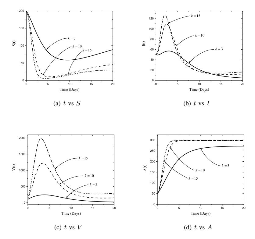
Figure 9: Impact of k on (1).
9. CONCLUSIONS
In this article, we study and analyze a delayed SIVA with-in host model of dengue virus transmission. R0 is computed using the NGM method. There are three different equilibrium states of (1), namely, VFE state E0, endemic equilibrium state without immune response E1 and EE state E2. We presented the stability dynamics of these states.
The VFE state E0 is l.a.s if R0 < 1 and unstable if R0 ≥ 1. For both the cases, τ = 0 and τ > 0, the stability criterion for E1 is also presented. For the given data in Table 2, we observe that E1 is l.a.s when τ = 0 and unstable when τ > 0. The EE state E2 is stable if it satisfies the condition (47) provided that M1 > 0, M2 > 0, and M4 > 0 for τ = 0. It is shown that E2 is stable for the given data in Table 2 when τ = 0. The critical value τ0 of the bifurcation parameter τ is derived for the endemic equilibrium E2. It may be noted that the System shows a stable nature when τ < τ0. But it exhibits a complex behavior and becomes unstable when τ > τ0. Thus it is concluded that a Hopf bifurcation occurs whenever τ > τ0.
The numerical simulation and sensitivity analysis of the System (1) is also presented and explained by graphs. The main contribution of this work are as follows:
- The R0 is evaluated using NGM method.
- The local stability of (1) is discussed and the stability condition is presented using the stability criterion of Lienard and Chipart for ´ τ = 0 and τ > 0.
- The endemic equilibrium E2 is stable when τ < τ0 and it exhibits Hopf bifurcation when τ > τ0.
- The sensitivity of the System (1) is also examined for various values of certain parameters.
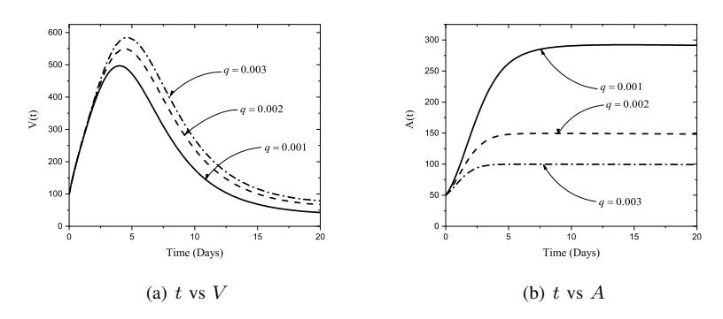
Figure 10: Impact of q on V and A.