

1. Introduction
Viral hepatitis is still one of life-threatening disease, which causes inflammation of liver, its all known five strains cause viral infection [2], [26], [14]. According to reports by world health organization (WHO), millions of people are infected with viral hepatitis, among them 354 million are suffering from chronic hepatitis B virus (HBV) and hepatitis C virus (HCV) globally, where 1.5 million and 1.575 million are new cases respectively in 2020 [26], [28]. Viral hepatitis is still a major public health burden, which is affecting millions of people with long-term complications [12], if it prolongs and be untreated then it could lead to liver cancer (Cirrhosis, liver fibrosis and hepatocellular carcinoma) and end-stage disease [18]. In highly endemic regions, most burden of HBV infection occurs in children with age less than equal to five years and those of individuals who are infected after age of five years develop to chronic infection [30]. Global mortality from viral hepatitis exceeds that of human immunodeficiency virus (HIV), tuberculosis (TB) and Malaria, both HBV and HCV are the most common cause of deaths with 1.3 million lives lost each year [27], [28]. Viral hepatitis is still a burden on world and threatens life of millions.
Many authors have investigated each strain and its dynamics individually, Mwaijande and Mpogolo [15] introduced a mathematical model for transmission dynamics of HAV with combined vaccination and sanitation, they incorporated direct and indirect transmission among humans with bi-linear incidence rate, revealed usual qualitative analysis and carried out sensitivity analysis of susceptible, exposed and infected individuals. They noted that vaccination and sanitation play important roles in minimizing future infection of viral hepatitis.
James et. al. [10] introduced a mathematical model on HBV and analysed its transmission dynamics in
*Corresponding author
Received April 1<sup>st</sup>, 2023, Revised May 5<sup>th</sup>, 2023 (first), Revised June 10<sup>th</sup>, 2023 (second), Accepted for publication June 28<sup>th</sup>, 2023. Copyright ©2023 Published by Indonesian Biomathematical Society, e-ISSN: 2549-2896, DOI:10.5614/cbms.2023.6.1.4
Nigeria, they appraised vaccination in the model, executed qualitative analysis at disease free equilibrium (DFE) and endemic points, as well as they studied impact of vaccination on population, eventually they recommended that every effort should be taken to reduce infection rate of the disease among population. Khatun et. al. [11] also worked out a mathematical model of HBV infection incorporating immune response, the model they introduced is SIV which is similar to SIR model. Further they incorporated the model with another equation for immune response z(t), they concentrated on studying dynamics of HBV among body cells and response of lymphocytes against hepatitis B pathogens.
Scott et. al. [20] introduced a deterministic SIS model with treatment for understanding transmission of HCV and effect of treatment on people who were injecting drugs. As well as Miller-Dickson et. al. [13] introduced a mathematical model on HCV as an indirectly transmitted infection, Bruno and Celso [4] developed a mathematical model for understanding analysis of Hepatitis Delta Virus (HDV) in vivo, they performed qualitative analysis, they discussed super-infection and co-infection which occur with existence of HBV. Yang et. al. [29] investigated feasibility of controlling hepatitis E virus(HEV) in Jiangsu province of China, they considered three routes of transmission of HDV in their model. They also estimated values of parameters, using curve fitting method and revealed the process of sensitivity of the model.
There are many other models, that study each strain individually, but there is no model for discussing all known strains of viral hepatitis. In the era of Covid19, viral hepatitis is ignored and the fact is that it is hazardous as Covid19. It still threatens life of millions of people and more than million people die each year because of it. This motivates us to catch up attention of responsible agencies, work hard for a safe and hepatitis free world, thus as an attempt we introduced a mathematical model focusing on dynamical behaviour of all known strains of viral hepatitis. Next generation matrix is calculated for determining its basic reproduction number (R0), local and global analysis at DFE point have been investigated, Minimum Mean Square Error (MMES) method is applied for obtaining values of involved parameters of the model. The estimation is based on the relevant data of viral hepatitis of Afghanistan for year 2020. Simulation of the model has been carried out, its numerical solution is plotted and One-at-a-time (OAT) sensitivity analysis is executed. We concluded that, sensitivity is due to infection rate of acute and chronic states of viral hepatitis, without any prevention measure, viral hepatitis could infect more than millions of people in the period of one year.
2. MODEL FORMULATION
In a typical model of dynamics of viral diseases, classes of population are considered. However, some practical assumptions are also made for simplifying the model. In our case, we compartmentalize the population, keeping various assumptions in view and formulating the dynamics of viral hepatitis.
| Table 1: Compartments and the corresponding variables. |
|---|
| Variables | Compartments |
|---|---|
| S(t) | Susceptible individuals (Age ≤ 5) |
| Y (t) | Susceptible individuals (Age > 5) |
| L(t) | Latent individuals |
| A(t) | Acute individuals |
| C(t) | Chronic individuals |
| R(t) | Removed individuals |
In this paper, two-age classes of susceptible population are considered as compartments S(t)&Y (t), this classification is based on immunity. Many age-structure models are formulated with Partial Differential Equations(PEDs), because of two continuous independent variables(age and time). However it can be formulated as ODE by considering anyone of the two variables as discrete. For further details of age-structure models, we referred section 7.5 of Mathematical Models in Population Biology and Epidemiology [1]. Age-structure models can also be formulated with the help of time-delay systems, further explanation can be found in [22] where the authors introduced a two-age-classes dengue transmission model, using time-delay systems.
In our case, age has been considered as discrete hence the dynamical behavior in each class is formulated with ODE, also it is assumed that the birth and death rates in S(t) and the death rate in Y (t) are constants, where the compartment S(t) includes those susceptible individuals, who are aged five years or less i.e. S(t) ≤ 5 and Y (t) includes susceptible individuals, who are aged greater than five years i.e. Y (t) > 5.
| Table 2: Parameters and meaning. | ||
|---|---|---|
| Parameters | Description |
|---|---|
| b | Recruitment rate |
| g | Rate of individuals who joins Y from S |
| µ | Death rate caused naturally |
| µ1 | Death rate caused by hepatitis |
| η1 | Infection rate by contacts between acute infectives and S |
| η2 | Infection rate by contacts between acute infectives and Y |
| β1 | Infection rate by contacts between chronic infectives and S |
| β2 | Infection rate by contacts between chronic infectives and Y |
| γ1 | Recovery rate of latent individuals |
| γ2 | Recovery rate of acute infectives |
| γ3 | Recovery rate of chronic infectives |
| ρ | Rate of latent individuals who become acute infectious |
| ρ1 | Severity reduction rate of chronic infectives |
| ω | Rate of acute infectives who develop to chronic stage |
| h | Probability of latent individuals showing symptoms |
| l | Probability of acute infectives who develop to chronic stage |
Parameters introduced in Table 2 are constants.
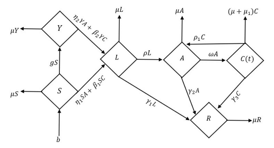
Figure 1: Flow chart of the model [2], [14], [16], [26].
Since the model focuses on all strains of viral hepatitis but the transmission routs are different for each strain, HAV and HEV are waterborne diseases they transmit via contaminated food and water. HBV, HCV and HDV have same transmission rout, they transmit via blood, semen and other body fluids, they can also be transmitted via pregnancy(Vertically). Since the model forecast outbreaks by viral hepatitis, so the transmission routes will not affect the outcome, hence for avoiding the complexity of vertical transmission, we assumed newborns as susceptible individuals and added into compartment S(t). As it is known, all strains of viral hepatitis have different incubation periods, so a compartment L(t) is considered for those individuals who are latent to the disease [30]. It is known, that viral hepatitis can be either acute or chronic [16], [14], [26], hence two compartments A(t) and C(t) are considered for acute and chronic individuals respectively, a compartment R(t) is considered for those individuals who recover from the infectious disease.
As stated above, the compartment S(t) contains individuals with age five years or less, these individuals grow up with constant rate g and are moving to compartment Y (t). It is obvious that, both infections either acute or chronic of viral hepatitis can cause new infections and the incidence rate in this paper is assumed to be bi-linear, therefore η1SA+β1SC of individuals from compartment S(t) are exposed by contacts with acute and chronic infectives, hence this dynamical behaviour is formulated in the differential equation below
\[\frac{dS}{dt} = b - (\eta_1 SA + \beta_1 SC) - (\mu + g)S,\tag{1}\]
where b is birth rate, µ is natural death rate and it is assumed to be constant for all compartments. Similarly, η2Y A + β2Y C individuals form Y become exposed by contact with acute and chronic infectives of viral hepatitis, so this dynamic is formulated as
\[\frac{dY}{dt} = gS - (\eta_2 YA + \beta_2 YC) - \mu Y. \tag{2}\]
Those susceptible individuals who became in contact with acute and chronic infectives are considered as latent and are added to L, some of these latent individuals may have good immune system against the disease, so they recover by themselves and those who develop symptoms are removed from it with constant rate ρ and probability h, so ρhL is the number of latent individuals who become acute infectious. Probability of those individuals who have good immune system is (1 − h) and they are assumed as recovered, then in this case the dynamic can be shown as
\[\frac{dL}{dt} = (\eta_1 S + \eta_2 Y)A + (\beta_2 S + \beta_2 Y)C - (\mu + \gamma_1 + h\rho)L.\] (3)
Individuals who become infectious are added to compartment A, as at the initial stage they are suffering from acute hepatitis, after a fixed course of treatment or vaccination individuals recover with constant rate γ2, also probability of those individuals who develop to chronic stage is l and are added to C with constant rate ω, so the dynamical behaviour in this case is formulated as
\[\frac{dA}{dt} = h\rho L + \rho_1 C - (\mu + \gamma_2) A - l\omega A. \tag{4}\]
Those of acute infectives who do not receive treatment or vaccine, develop to chronic stage with constant rate ω. In this stage, deaths caused by disease occur with constant rate µ1, as well in case of complete course of treatment, the risk of severity reduces and chronic infectives switch back to acute stage with constant rate ρ1, so mathematically this dynamical behaviour is expressed as
\[\frac{dC}{dt} = l\omega A - (\mu + \mu_1 + \rho_1 + \gamma_3)C. \tag{5}\]
Recovered individuals from latent, acute and chronic stages are γ1L, γ2A and γ3C respectively, so this can be formulated as
\[\frac{dR}{dt} = (1 - h)\gamma_1 L + \gamma_2 A + \gamma_3 C - \mu R. \tag{6}\]
Dynamical behaviour of viral hepatitis, which is depicted in Figure (1) is formulated in Equations (1 - 6) and all these equations together form a system of non-linear differential equations, where it is the expected model.
Total population size of the model is N = S + Y + L + A + C + R, where S > 0, Y > 0, L ≥ 0, A > 0, C > 0 and R ≥ 0. As it may vary in time, hence rate of change of the population of above model is given as differential equation below.
\[\frac{d}{dt}(S+Y+L+A+C+R) = \mu(S+Y+L+A+C+R) - \mu_1 C - h\gamma_1 L. \tag{7}\]
In the absence of disease, total population size of the model converges to the equilibrium point x0, where it is known as DFE (see [24]).
\[x_0 = (S^*, Y^*, L^*, A^*, C^*, R^*) = (\frac{b}{\mu + g}, \frac{bg}{\mu(\mu + g)}, 0, 0, 0, 0).\] (8)
3. BASIC REPRODUCTION NUMBER \((R_0)\)
Since \(x_0\) in (8) is the DFE point of the system, hence the basic reproduction number \((R_0)\) at \(x_0\) can be found by next-generation matrix introduced by Driessche and Watmough [25] and its application can be found in [21]. As R does not have role in infection of population, then it is ignored and the first five equations of the system are considered for further analysis.
Let \(X = (L, A, C, S, Y)^T\), then Equations (1 - 6) can be considered as X' = f(X). Now distinguishing newly infected individuals from all others in population, therefore
\[X' = \frac{dX}{dt} = \mathcal{F}(x) - \mathcal{V}(x),\] where \(\mathcal{F}(X)\) is the rate of newly infected individuals, \(\mathcal{V}(X) = \mathcal{V}^{-}(X) - \mathcal{V}^{+}(X)\) is rate of transfer of individuals in compartments and they are given as
\[\mathcal{F}(x) = \left[ \begin{array}{c} (\eta_1 S + \eta_2 Y) A + (\beta_1 S + \beta_2 Y) C \\ 0 \\ 0 \\ 0 \end{array} \right] \qquad \& \qquad \mathcal{V}(x) = \left[ \begin{array}{c} (\mu + \gamma_1 + h\rho) L \\ -h\rho L - \rho_1 C + (\mu + \gamma_2 + l\omega) A \\ -l\omega A + (\mu + \mu_1 + \rho_1 + \gamma_3) C \\ -b + (\eta_1 SA + \beta_1 SC) + (\mu + g) S \\ -gS + (\eta_2 YA + \beta_2 YC) + \mu Y \end{array} \right].\]
Here \(\mathcal{V}^+(X)\) is the rate of transfer of individuals into compartments and \(\mathcal{V}^-(X)\) is the rate of transfer of individuals out of compartment.
Let \(X_s = \{x \ge 0 \mid x_0 = 0, i = 1, 2, 3, 4, 5\}\) be set of all disease-free states. Since, \(x_0\) is DFE of the system and f(X) satisfies the conditions below.
- 1) \(\mathcal{F}_i(x_0), \ \mathcal{V}^-(x_0), \ \mathcal{V}^+(x_0) \ge 0 \text{ for } i=1,2,...,n \text{ if } x_0 \ge 0 \text{ and } n=5.\)2) \(\mathcal{V}^-(x_0) = 0 \text{ and } \mathcal{F}_i(x_0) = 0 \text{ for } i=1,2,...,m \text{ if } x_0 = 0 \text{ and } m=5.\)
- 3) \(\mathcal{F}_i(x_0) = 0 \text{ if } i > 5.\)
Hence the derivatives \(D\mathcal{F}\left(X_{0}\right)\) and \(D\mathcal{V}\left(X_{0}\right)\) can be partitioned as
\[D\mathcal{F}\left(X_{0}\right)=\left[\begin{array}{cc}F&0\\0&0\end{array}\right]\qquad\&\qquad D\mathcal{V}\left(X_{0}\right)=\left[\begin{array}{cc}V&0\\J_{1}&J_{2}\end{array}\right],\] where F and V are \(3 \times 3\) matrices, as the system has three disease states. Furthermore, F is nonnegative, V is nonsingular M-matrix and \(J_2\) has eigenvalues \((\mu, \mu + g)\), where \(\mu, g > 0\), given as
\[F = \left[\frac{\partial \mathcal{F}_i}{\partial X_j}(x_0)\right] \& F = \left[\frac{\partial \mathcal{V}_i}{\partial X_j}(x_0)\right], \text{ with } i = 1, 2, 3 \text{ and } j = 1, 2, 3, \text{ hence we have } i = 1, 2, 3, i = 1, 2, 3, \dots\]
\[F = \begin{pmatrix} 0 & \frac{b(\mu\eta_1 + g\eta_2)}{\mu(\mu + g)} & \frac{b(\mu\beta_1 + g\beta_2)}{\mu(\mu + g)} \\ 0 & 0 & 0 & 0 \\ 0 & 0 & 0 & 0 \end{pmatrix},\] \[V = \begin{pmatrix} \mu + \gamma_1 + h\rho & 0 & 0 \\ -h\rho & \mu + \gamma_2 + l\omega & -\rho_1 \\ 0 & -l\omega & \mu + \mu_1 + \rho_1 + \gamma_3 \end{pmatrix}.\] (9)
Assuming, that all exposed individuals are showing symptoms and become infected, moreover none of chronic infected individual turn back to acute stage, as they acquire treatment, then
\[V = \begin{pmatrix} \mu + h\rho & 0 & 0 \\ -h\rho & \mu + \gamma_2 + l\omega & 0 \\ 0 & -l\omega & \mu + \mu_1 + \gamma_3 \end{pmatrix},\](10)
then
\[V^{-1} = \begin{pmatrix} \frac{1}{\mu + h\rho} & 0 & 0\\ \frac{h\rho}{(\mu + h\rho)(\mu + l\omega + \gamma_2)} & \frac{1}{\mu + l\omega + \gamma_2} & 0\\ \frac{hl\rho\omega}{(\mu + h\rho)(\mu + l\omega + \gamma_2)(\mu + \gamma_3 + \mu_1)} & \frac{l\mu\omega + hl\rho\omega}{(\mu + h\rho)(\mu + l\omega + \gamma_2)(\mu + \gamma_3 + \mu_1)} & \frac{1}{(\mu + \gamma_3 + \mu_1)} \end{pmatrix}.\](11)
Next generation matrix of the system is
\[FV^{-1} = \begin{pmatrix} p & q & r \\ 0 & 0 & 0 \\ 0 & 0 & 0 \end{pmatrix}, \tag{12}\]
where
\[p = \frac{bh\rho(l\mu\omega\beta_1 + gl\omega\beta_2 + (\mu\eta_1 + g\eta_2)(\mu + \gamma_3 + \mu_1))}{\mu(g + \mu)(\mu + h\rho)(\mu + l\omega + \gamma_2)(\mu + \gamma_3 + \mu_1)},\] \[q = \frac{b(l\mu\omega\beta_1 + gl\omega\beta_2 + (\mu\eta_1 + g\eta_2)(\mu + \gamma_3 + \mu_1))}{\mu(g + \mu)(\mu + l\omega + \gamma_2)(\mu + \gamma_3 + \mu_1)},\] \[r = \frac{b(\mu\beta_1 + g\beta_2)}{\mu(g + \mu)(\mu + \gamma_3 + \mu_1)}.\]
The basic reproduction number at DFE point is the spectral radius of next generation matrix, which is the entry p in Matrix (12), it is usually denoted as \(R_0\), given below;
\[R_0 = \frac{bh\rho(l\mu\omega\beta_1 + gl\omega\beta_2 + (\mu\eta_1 + g\eta_2)(\mu + \gamma_3 + \mu_1))}{\mu(g+\mu)(\mu + h\rho)(\mu + l\omega + \gamma_2)(\mu + \gamma_3 + \mu_1)},\] (13)
where l and h are probabilities of acute infectives who develop to chronic stage and latent individuals showing symptoms respectively with \(0 \le l \le 1\) and h = 1 as all exposed are assumed to show symptoms but for general case h must be \(0 < h \le 1\). If \(R_0 < 1\), then on average a hepatitis infected individuals infect less than one individual from population over the course of its infectious period, thus infection is under control and stable. Also, if \(R_0 > 1\), then hepatitis invades population and more than one individual can be infected over course of infection period.
For asymptotic local stability of the system, recalling the definitions of Z-matrix and M-matrix, given by [7], and proving the below result given in [21], [25].
Theorem 3.1. Considering model (1 - 6) of viral hepatitis, if \(x_0\) be DFE point of the model, then it is locally asymptotically stable if \(R_0 < 1\) but unstable if \(R_0 > 1\), where \(R_0\) is defined in (13).
Proof: To prove locally asymptotically stability of the DFE point, using matrices (9) and (10) respectively as P = F - V. Since V is Z-matrix with eigenvalues whose real parts are non-negative, it is non-singular M-matrix, F is also non-negative and V - F = -P has Z-pattern too, then 1. Let s(P) < 0.
Since spectral abscissa s(P)<0, it implies that -P is a non-singular M-matrix. Let \(-PV^{-1}=I-FV^{-1}\), since -P has Z-pattern and it is non-singular M-matrix, hence \(-PV^{-1}\) is non-singular M-matrix and moreover \(I-FV^{-1}\) is non-singular M-matrix, it is clear that \(FV^{-1}\) given in (12) is a non-negative matrix and all its eigenvalues have magnitude less than or equal to \(\rho(FV^{-1})\), also we know that maximum eigenvalue of Matrix (12) is known as basic reproduction number(\(R_0\)), i. e. \(R_0=\rho(FV^{-1})\). Since \(I-FV^{-1}\) is a non-singular M-matrix, so it implies that;
\[\begin{split} & \rho(FV^{-1} - I) < 0, \\ & \rho(FV^{-1}) - \rho(I) < 0, \\ & \rho(FV^{-1}) - 1 < 0, \\ & \rho(FV^{-1}) < 1, \\ & R_0 < 1, \end{split}\] : (I is identity matrix.)
It can be concluded that, s(P) < 0 iff. \(R_0 < 1\).
2. Let s(P) = 0.
Since spectral abscissa s(P) is zero, it implies that -P is a singular M-matrix, therefore \(I - FV^{-1}\) is a singular M-matrix too, thus \(\rho(FV^{-1}) = 1\), i.e. \(R_0 = 1\) hence s(P) = 0 iff. \(R_0 = 1\).
3. Let s(P) > 0. By above two cases, it follows that s(P) > 0 iff. \(R_0 > 1\), which is as given in (13).
Now for global stability, it is necessary to determine feasible region of the system.
3.1. Feasible Region
Feasible region is the set of all possible solutions of a system of equations, to determine it for model (1 - 6), adding equations \(\frac{dS}{dt}\), \(\frac{dY}{dt}\), \(\frac{dA}{dt}\) and \(\frac{dC}{dt}\), we get
\[\frac{d}{dt}(S+Y+L+A+C) = b - \mu(S+Y+L+A+C) - \mu_1 C - \gamma_1 L - \gamma_2 A - \gamma_3 C.\]
Here \(\gamma_1 = 0\), as it has been assumed that all the latent individuals are with symptoms, also for short time period epidemic, loss of temporary immunity can be assumed to be negligible, so the equation turns down to inequality below.
\[\frac{d}{dt}(S+Y+L+A+C) \le b - \mu(S+Y+L+A+C).\]
For determining upper bound of the region taking \(\limsup_{t\to\infty}(S+Y+L+A+C)\leq \frac{b}{\mu}\), so we obtain feasible region of the model (1 - 6) as
\[\phi = \left\{ (S, Y, L, A, C) \in \mathbb{R}^{+5} : S + Y + L + A + C \le \frac{b}{\mu}, S > 0, Y > 0, L \ge 0, A > 0, C > 0 \right\}. \tag{14}\]
For global stability of the introduced model, we refer to a similar result obtained by Zada et. al. [30] as below.
Theorem 3.2. Model (1 - 6) is globally asymptotically stable at disease free equilibrium point, if there is at least continuously differentiable function \(V: \phi \to \mathbb{R}\), such that V be positive definite and V' be negative definite (semi definite) function in \(\phi\), otherwise it is unstable.
Proof: In order to prove global stability of the model , constructing a simple Lyapunov function \(V:\phi\to\mathbb{R}\) as
\[V(t) = S(t) + Y(t) + L(t) + A(t) + C(t).\] (15)
Using definition of positive definiteness [17] to verify that V is a positive definite function, now by derivative of V, we get
\[\frac{dV}{dt} = \frac{\partial V}{\partial S} \frac{dS}{dt} + \frac{\partial V}{\partial Y} \frac{dY}{dt} + \frac{\partial V}{\partial L} \frac{dL}{dt} + \frac{\partial V}{\partial A} \frac{dA}{dt} + \frac{\partial V}{\partial C} \frac{dC}{dt},\] \[\Rightarrow \frac{dV}{dt} = \frac{dS}{dt} + \frac{dY}{dt} + \frac{dL}{dt} + \frac{dA}{dt} + \frac{dC}{dt}.\] (16)
Therefore.
\[V' = \frac{dV}{dt} = -[-b + \mu S + \mu Y + (\mu + \gamma_1)L + (\mu + \gamma_2)A + (\mu + \mu_1 + \gamma_3)C].\]
Using definition of negative semi definiteness, the definition makes it is easy to verify that V' is negative semi definite at \(x_0\), hence by LaSalle's theorem [17], it implies that the model (1 - 6) is globally asymptotically stable at disease free equilibrium point and unstable if there is not at least one positive definite function V.
4. SIMULATION
In this section, relevant data of Afghanistan for the year 2020 is represented, visualized in Figure 2, where Figure 2(a) shows morbidity and mortality by each strain of viral hepatitis in 2020 and Figure 2(b) shows total number of infectives in consideration with age of individuals, number of acute and chronic individuals.
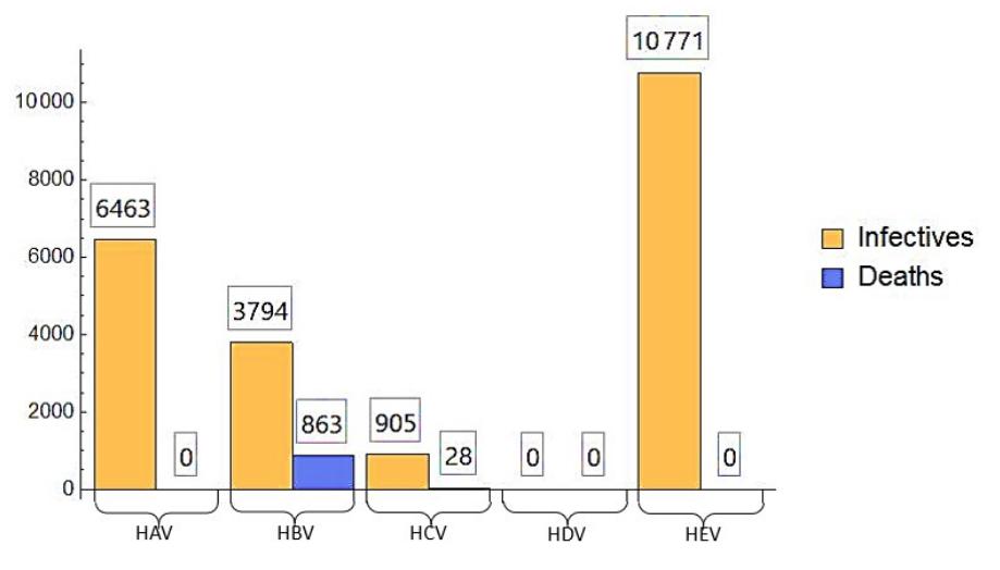
(a) Total number of infctives and deaths, caused by each strain.
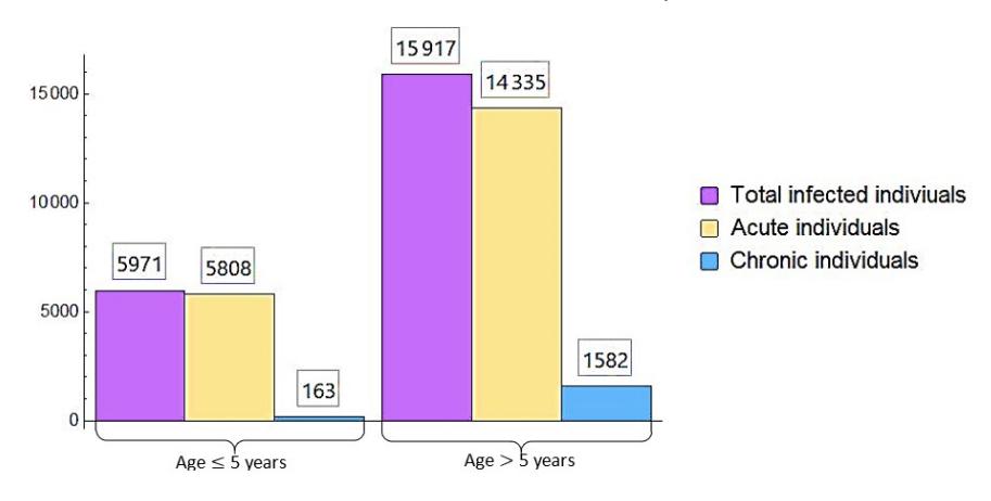
(b) Total number of infected individuals according to age and disease severity.
Figure 2: Viral hepatitis relevant data, available for Afghanistan in the year 2020. [19].
4.1. Estimation
For convenient calculation, it is assumed that no chronic individual becomes acute back, either they recover or die, so \(\rho_1=0\) and all of latent individuals declare symptoms, so \(\gamma_1=0\). For estimation of parameters \(b,g,\mu,\mu_1,\eta_1,\eta_2,\beta_1\) and \(\beta_2\), see Appendix A. For remaining parameters of the model, we have compared estimators that have been optimized using two different estimators; the Minimum MSE (Mean Squared Error) Estimator and the Minimum MAE (Mean Absolute Error) Estimator. The algorithm has been applied on \(\frac{dA}{dt}\) for estimating the unknown involved parameters \(\rho,\gamma_2\) and \(\omega\), where the algorithms are given as
A. MMSE Estimator:
- Input changes of confirmed cases of acute infectives at time t (Monthly) i.e. \(\frac{dA}{dt}\).
- Assigning initial values of the parameters at their respective ranges \(\theta = [\rho, \gamma_2, \omega]^T\).
- 3) Computing values of
\[\widehat{\frac{dA}{dt}} = \rho L + \rho_1 C - (\mu + \gamma_2) A - l\omega A,\]
using arbitrary initial values \(\hat{\theta}\). 4) Comparing the values of \(\frac{dA}{dt}\) with computed values in the equation, by computing MSE as;
\[MSE\left(\widehat{\frac{dA}{dt}}\right) = \frac{1}{n} \sum_{i=1}^{n} \left(\frac{dA}{dt} - \frac{\widehat{dA}}{dt}\right)^{2}.\]
5) Computing the gradient of the MSE jointly for all parameter estimates by solving the equation
\[\nabla_0 MSE\left(\frac{\widehat{dA}}{dt}\right) = 0, \theta = \left[\rho, \gamma_2, \omega\right]^T,\] so we obtain new estimates of \(\theta\).
Repeat steps 4 - 6, until MSE converges to a desirable small value.
B. MMAE Estimator: In this method, all the mentioned steps of MMSE method can be followed with small change in step 4 as;
\[MAE\left(\widehat{\frac{dA}{dt}}\right) = \frac{1}{n} \sum_{i=1}^{n} \left| \frac{dA}{dt} - \frac{\hat{dA}}{dt} \right|.\]
The MMAE estimator gives accurate and desirable result than MMSE estimator, hence the remaining parameters are estimated using MMAE method with the help of R-programming, where R-code of the function is available in Appindex B and the estimated values of the parameters are given in Table 3.
Table 3: Values of the parameters 2, estimated from data given in Figure 2.
| Parameters | Estimation | Unit | Source |
| \(\overline{}\) | 0.124913 | \(Month^{-1}\) | Assumed |
| g | 0.1244 | \(Month^{-1}\) | Estimated |
| \(\mu\) | 0.000513 | _ | Cited [9] |
| \(\mu_1\) | 0.04255 | \(Month^{-1}\) | Estimated |
| \(\eta_1\) | 0.00214 | \(Month^{-1}\) | Estimated |
| \(\eta_2\) | 0.000458 | \(Month^{-1}\) | Estimated |
| \(\beta_1\) | 0.000141 | \(Month^{-1}\) | Estimated |
| \(\beta_2\) | 0.0000456 | \(Month^{-1}\) | Estimated |
| \(\gamma_1\) | 0 | _ | Assumed |
| \(\gamma_2\) | 0.9983 | \(Month^{-1}\) | Estimated |
| \(\gamma_3\) | 0.456 | \(Month^{-1}\) | Estimated |
| \(\rho\) | 0.442 | \(Month^{-1}\) | Estimated |
| \(\rho_1\) | 0 | _ | Assumed |
| \(\omega\) | 0.0006162 | \(Month^-\) | Estimated |
Since h = 1 and \(0 \le l \le 1\), then basic reproduction number \(R_0\) given in (13), is between 0.113206 and 0.112649, i.e. \(R_0 < 1\), hence by Theorem 3.1 viral hepatitis is asymptotically stable and was under control. The system of Equations (1 - 6) was then solved numerically, using Wolframe Mathematica (command: NDSolve), which chooses appropriate method and giving interpolating functions as output, to estimate the effect on total number of both acute and chronic individuals of viral hepatitis.
Since the solution changes with the value of l, therefore solutions at different values of l are shown in the figures below. If l = 0, then transmission of the disease would be as shown in Figure 3, that implies that there would be no new infection of chronic individuals and current infected individuals will either die out or attain recovery, as shown in Figure 4.
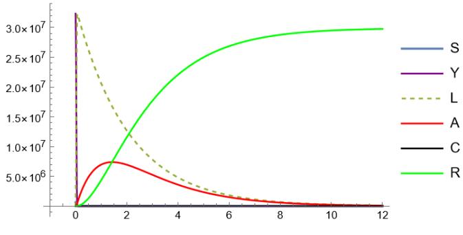
Figure 3: solution at l = 0.
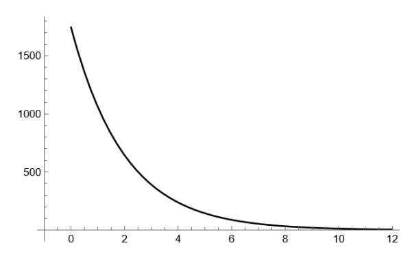
Figure 4: Total number of chronic infectives when l = 0.
Number of infected individuals have been observed to increase and the value of l changes in the range 0 ≤ l ≤ 1. If value of l = 0.5, then variation can be seen in Figures 5 and 6. Also total chronic individuals are estimated to be about 8000.
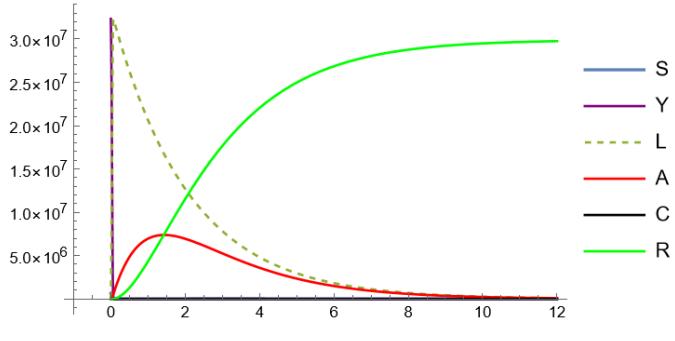
Figure 5: Solution at l = 0.5.
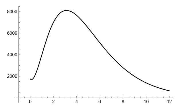
Figure 6: Total number of chronic infectives when l = 0.5.
Moreover, the interaction between all the compartments and variations at l = 1 can be observed in Figure 7, total chronic individuals are at peak and are estimated to be about 15000, which is shown in Figure 8.
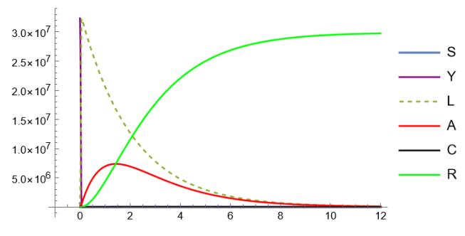
Figure 7: Solution at l = 1.
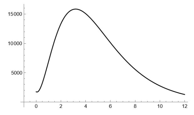
Figure 8: Total number of chronic infectives when l = 1.
It is obvious that viral hepatitis is an infectious disease and in the Figures 3, 5 and 7, it is also visible that without any prevention strategy, the whole population is exposed. From simulation, it can also be observed that the infection rate depends on number of acute and chronic infections, it increases if total number of acute and chronic infectives increases. To take control over infection rate and avoid new infections, it is suggested to concentrate on the routes through which they spread.
4.2. Sensitivity Analysis
It is known that, each model has factors of sensitivity. Investigation of such factors is known as sensitivity analysis, that is useful in determination of parameters of models which are the most responsible for changes in dynamics of the systems. There are various methods of sensitivity analysis, which include differential sensitivity analysis, One-at-a-time sensitivity analysis (OAT method), Subjective sensitivity analysis and so on. Each method of sensitivity analysis focuses on different aspects of dynamics of the phenomena [8], these methods are brought into use by various researchers, a valuable application of differential sensitivity analysis can be found in the literature by Tay et.al. [23], and Fakhruddin et.al. [5]. In our case we executed OAT method, in which a single parameter is taken into consideration at a time to see its effect on output, which is helpful in determination of effect on dynamics of viral hepatitis by each parameter. For the considered model of viral hepatitis each parameter is varied for investigating variability and impact on output of the model, we have considered the parameters ρ and ω as the most sensitive parameters of the model, where these parameters represent rate of latent individuals who become acute infectives and rate of acute infectives transforming to chronic stage respectively. Our analysis shows that these are significant sensitivity parameters, as it can be seen in the Figs 9 and 10.
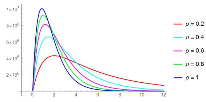
Figure 9: Graph of acute infectives represented by parameter ρ at values 0.2, 0.4, 0.6, 0.8 and 1.
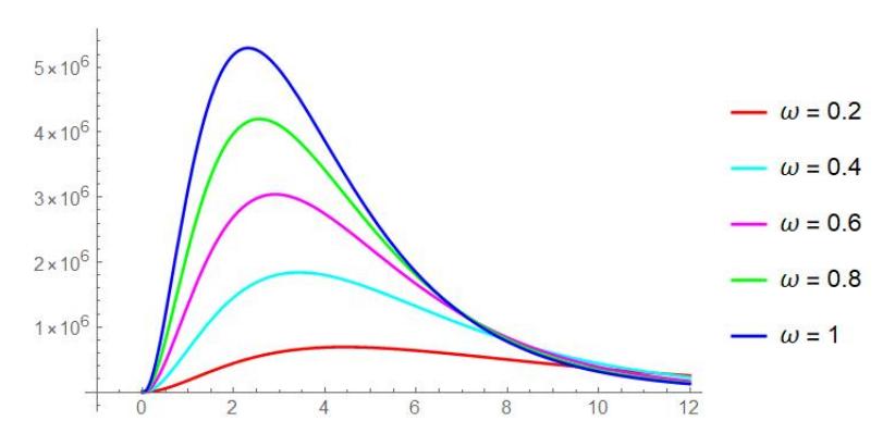
Figure 10: Graph of chronic infectives represented by parameter ω at values 0.2, 0.4, 0.6, 0.8 and 1.
5. CONCLUSION
Many authors have investigated behaviour of various strains of viral hepatitis individually and some of them investigated super infection and co-infection of HBV-HDV, but there is no any model to predict overall number of infections by viral hepatitis (All known strains). In this paper we formulated transmission dynamics of all the known strains of viral hepatitis in one frame and proposed a deterministic model. Qualitative analysis of the model at disease free equilibrium point has been performed. For simulation, data of viral hepatitis of Afghanistan for the year 2020 is taken into focus, values of all the parameters are estimated based on probabilities, as well as by using the method of Minimum MAE estimator in comparison with Minimum MSE estimator, it has been concluded that MAE estimator gives accurate and desirable small values of parameters. Numerical solution is plotted and calculations of the model are carried out with the help of Wolfram Mathematica. One- At- a – Time (OAT) method of sensitivity is applied for determining significant parameters, it has been noticed that sensitivity of the model depends on infection rates of acute and chronic viral hepatitis. As output of the model suggests, that entire population of Afghanistan could become affected if no prevention measures were taken by responsible agencies. Total number of infected individuals caused by viral hepatitis is considerably high but ignored by responsible agencies. To know severity of viral hepatitis and engage the agencies for its prevention, so this model can help us predict outbreak by all strains of viral hepatitis.
ACKNOWLEDGMENTS
BS is thankful to Indian Council of Cultural Relations(ICCR), Department of External Affairs - Government of India, New Delhi, who is sponsoring his Ph.D. We are also thankful to Dr. Mohammad Rafiq Safi, Mr. Viral Patel and Mr. Sagar V Soni, who helped in the preparation of manuscript, as well as we are thankful to referees for their critical remarks which helped in improving the manuscript.
Appendix A
Parameters \(b, g, \mu, \mu_1, \eta_1, \eta_2, \beta_1\) and \(\beta_2\) are estimated as;
\[g = \frac{\text{Total number of childern who aged} \leq 5 \text{ years}}{\text{Total number of children with birtdays} \times \text{Time}} = \frac{1316159}{881671 \times 12M} = 0.1244 \ \ M^{-1}.\]
\(\mu=\frac{6.16}{1000\times 12M}=0.000513~M^{-1}\) is cited from [9]. Recruitment rate b in compartment S is assumed to be equal to the exit rate from S, so the parameter is estimated as \(b=\mu+g=0.124913~M^{-1}\).
\[\mu_1 = \frac{\text{Total number of deaths by disease}}{\text{Total number of chronic infectives} \times \text{Time}} = \frac{891}{1745 \times 12M} = 0.04255 \ M^{-1}\] \[\eta_1 = \frac{\text{Number of acute infected individuals }(A)}{\text{Number of contacts by } A \text{ with } S \times \text{Time}} = \frac{20143}{784384(assumed) \times 12M} = 0.00214 \ M^{-1}\] \[\beta_1 = \frac{\text{Number of chronic infected individuals }(C)}{\text{Number of contacts by } C \text{ with } S \times \text{Time}} = \frac{1745}{1030690(assumed) \times 12M} = 0.000141 \ M^{-1}\] \[\eta_2 = \frac{\text{Number of acute infected individuals }(A)}{\text{Number of contacts by } A \text{ with } Y \times \text{Time}} = \frac{20143}{3665029(assumed) \times 12M} = 0.000458 \ M^{-1}\] \[\beta_2 = \frac{\text{Number of chronic infected individuals }(C)}{\text{Number of contacts by } C \text{ with } Y \times \text{Time}} = \frac{1745}{3188961(assumed) \times 12M} = 0.0000456 \ M^{-1}\]
Appendix B
1) R-code of MSE function:
### params < - [rho, gamma2, omega] \
MSE < - function(params){
    dA_ hat < - params[1]*vL + rho1*vC - (mu + params[2]*vA - 1*params[3]*vA return(sum((dA - dA_ hat)^ 2 ))
    }
    initial < - c(0.1, 0.1, 0.1)
    optim(initial, MSE, method = "BFGS")

Output: [0.07793074, 0.12221979, 0.02110990]
2) R-code of MAE function :
    MAE < − function(params){
    dA hat < − params[1]*vL + rho1*vC - (mu + params[2]*vA - l*params[3]*vA
    return(sum((dA - dA hat)ˆ 2 ))
    }
    initial < − c(0.1, 0.1, 0.1)
    optim(initial, MAE, method = "BFGS-B", upper = 1)
Output: [0.4420848964, 0.9983098068, 0.0001612701]
Same algorithm and the above R-code can be used for other equations and involved parameters.