

1. Introduction
In recent decades, mathematical modelling of predator-prey interaction has attracted enormous interest from researchers and has been rapidly developed. Among the developments may applied the assumptions of the existing of harvesting [17], [24], [13], spread of disease [15], [11], Allee effect [16], [27], and stage-structure [5], [26]. Another interesting development is by adding the assumption of cannibalism existence [19]. The following model is a predator-prey model involving cannibalism in predator proposed by Deng et al [8].
\[\frac{dN}{dt} = rN\left(1 - \frac{N}{K}\right) - b_1 NP,\] \[\frac{dP}{dt} = c_1 NP + c_2 P - eP - \frac{b_2 P^2}{k_2 + P}.\] (1)
\(N \ge 0\) and \(P \ge 0\) in (1) are the size population of prey and predator, respectively. In the absence of predator, prey grows logistically with a rate of r and the environment's carrying capacity of K. Then, in the presence of predator, prey decreases by \(b_1NP\) which is a type I Holling functional response with the predation rate of \(b_1\). Prey biomass consumed by predator is converted into predator births at a rate of \(c_1\). The predator dies naturally at a rate of e and decreases due to cannibalism by \(\frac{b_2P^2}{k_2+P}\), with \(b_2\) and \(k_2\) denote the maximum cannibalism rate and half-saturation constant of cannibalism, respectively. The cannibalism is converted to predator birth linearly at a rate of \(c_2\).
<sup>2</sup>Department of Mathematics Education, Faculty of Pedagogy and Psychology, PGRI Wiranegara University, Pasuruan 67118, Indonesia
*Corresponding author
Received January \(3^{rd}\), 2023, Revised February \(25^{th}\), 2023 (first), Revised April \(10^{th}\), 2023 (second), Accepted for publication May \(5^{th}\), 2023. Copyright ©2023 Published by Indonesian Biomathematical Society, e-ISSN: 2549-2896, DOI:10.5614/cbms.2023.6.1.2
The system (1) had been modified by changing the predation rate following the type II Holling functional response and adding the assumption of the cannibalized predator refuge [18]. The modified system is
\[\frac{dN}{dt} = rN\left(1 - \frac{N}{K}\right) - \frac{b_1 N P}{k_1 + N}, \frac{dP}{dt} = \frac{c_1 N P}{k_1 + N} + c_2 P - eP - \frac{b_2 (1 - m) P^2}{k_2 + (1 - m) P},\] (2)
with \(k_1\) denotes half-saturation constant of predation and m is proportion of refuge, while \(b_1\) becomes the maximum predation rate. The dynamical properties of (2), those are the existence of equilibrium points, local and global stability analysis of the equilibrium points, and forward bifurcation existence had been shown in [18].
The predator-prey model (2) is a continuous dynamic system which is in the form of a system of nonlinear differential equations. Meanwhile, in general, nonlinear differential equations system cannot be solved analytically. Hence, discretization is required for approximating their solutions [3]. Moreover, as the stability of the equilibrium points in discrete models typically depends on the integration time stepsize, the discrete model mostly results in richer dynamics than the continuous one [9], [25].
A discrete model of a system of first-order differential equations can be obtained by applying the discretization method. Euler's method is one of the simplest method to discretize systems of differential equations. However, Mickens [12] had shown that the Euler discretization method has a weakness, that is the numerical instability. To eliminate it, Mickens proposes another method, namely the Nonstandard Finite Different (NSFD) scheme. By adopting the exact finite difference scheme, NSFD becomes a generalization of the Euler scheme. The most important property of a NFSD is that, in most cases, it eliminates the instability of the Euler scheme. NSFD follows the rules described below [12].
The first derivative of the differential equations system is approximated by the generalization of Euler's forward difference scheme, i.e
\[\frac{dX(n)}{dt} \to \frac{X(n+1) - X(n)}{\phi},\] with X(n) = X(t(n)), \(\phi = \phi(h)\) is a denominator function such that \(\phi(h) = h + O(h^2)\), and h is the integration time step size.
2) The nonlinear form must be replaced with a non-local form like the following examples.
\[X^2 \to X(n+1)X(n),\] \(XY \to \frac{X(n+1)+X(n-1)}{2}Y(n),\) etc.
If a discrete model and its corresponding continuous model have the same dynamic properties, they are said to be dynamically consistent [2]. The consistency of dynamics can be obtained using the discretization method of NFDS. NSFD has also been applied by researchers recently to develop biomathematics models into discrete systems [21], [6], [10], [1], [23], [7], [4], [14]. Therefore, in this paper, a NSFD scheme used to study discrete dynamical system of predator-prey model involving cannibalism and refuge in predator.
2. MODEL DEVELOPMENT
The continuous differential equation system (2) is discretizated as follows.
\[\begin{array}{ccc} N^2 & \to & N(n+1)N(n), \\ NP & \to & N(n+1)P(n), \\ P^2 & \to & P(n+1)P(n), \\ \frac{dN}{dt} & \to & \frac{N(n+1)-N(n)}{\phi(h)}, \\ \frac{dP}{dt} & \to & \frac{P(n+1)-P(n)}{\phi(h)}, \end{array} \tag{3}\] where the denominator function \(\phi(h)\) is \(\phi(h) = h\). Through the discretization, the nonstandard numerical scheme for the system (2) is
\[N(n+1) = N(n) + h\left(rN(n)\left(1 - \frac{N(n+1)}{K}\right) - \frac{b_1N(n+1)P(n)}{k_1 + N(n)}\right),\] \[P(n+1) = P(n) + h\left(\frac{c_1N(n+1)P(n)}{k_1 + N(n)} + c_2P(n) - eP(n+1) - \frac{b_2(1-m)P(n+1)P(n)}{k_2 + (1-m)P(n)}\right).\] (4)
By using some algebraic manipulations, we get the explicit form for System (4), i.e.
\[N(n+1) = \frac{N(n)(1+hr)}{\left[1+h\left(\frac{rN(n)}{K}+\frac{b_1P(n)}{k_1+N(n)}\right)\right]} \equiv G_1(N(n),P(n)),\] \[P(n+1) = \frac{P(n)}{\left[1+h\left(e+\frac{b_2(1-m)P(n)}{k_2+(1-m)P(n)}\right)\right]} \left(1+\frac{hc_1N(n)(1+hr)}{(k_1+N(n))\left[1+h\left(\frac{rN(n)}{K}+\frac{b_1P(n)}{k_1+N(n)}\right)\right]} + hc_2\right) \equiv G_2(N(n),P(n)).\] (5)
To investigate the local stability of the equilibrium points of the system (3), the following lemma is very useful.
Lemma 2.1. [22] Consider \(E^* = (N^*, P^*)\) is an equilibrium point of a two dimensional discrete system. For the quadratic equation \(\lambda^2 - \tau(J(E^*))\lambda + \Delta(J(E^*)) = 0\), the roots satisfy \(|\lambda_i| < 1, \forall i = 1, 2\), if and only if all of the following conditions are satisfied.
- 1) \(1 + \tau(J(E^*)) + \triangle(J(E^*)) > 0\):
- 2) \(1 \tau(J(E^*)) + \triangle(J(E^*)) > 0\);
- 3) \(\triangle(J(E^*)) < 1\);
where \(\tau(J(E^*))\) and \(\Delta(J(E^*))\), respectively, are the trace and determinant of characteristic equation of the Jacobian matrix at \(E^*\).
3. LOCAL STABILITY
The equilibrium points of system (3) are obtained by finding the solutions of
\[G_1(N(n), P(n)) = N(n),\]
\(G_2(N(n), P(n)) = P(n),\)
which is equivalent to the following system.
\[rN^* \left( 1 - \frac{N^*}{K} \right) - \frac{b_1 N^* P^*}{k_1 + N^*} = 0,\]
\[\frac{c_1 N^* P^*}{k_1 + N^*} + c_2 P^* - eP^* - \frac{b_2 (1 - m) P^{*2}}{k_2 + (1 - m) P^*} = 0.\]
The equilibrium points are:
- The origin, E<sub>0</sub>(0,0), that clearly exists in R<sup>2</sup><sub>+</sub> = {(N, P) : N ≥ 0, P ≥ 0}. The prey extinction point, E<sub>1</sub> (0, (k<sub>2</sub>(e c<sub>2</sub>))/((c<sub>2</sub> e b<sub>2</sub>)(1 m)), that exists in R<sup>2</sup><sub>+</sub> if 0 < c<sub>2</sub> e < b<sub>2</sub>. The predator extinction point, E<sub>2</sub>(K,0). E<sub>2</sub> always exists in R<sup>2</sup><sub>+</sub> since K > 0.
- 4) The coexistence point, \(E_3(N_3, P_3)\). If \(b_2 + e \neq c_1 + c_2\), \(N_3\) and \(P_3\) are derived by Cardanos's formula in [20] i.e
\[N_{3} = \frac{\sqrt[3]{Q_{2} \pm \sqrt{Q_{2}^{2} + \frac{4}{27}Q_{1}^{3}}}}{\sqrt[3]{2}} - \frac{Q_{1}\sqrt[3]{2}}{3\sqrt[3]{Q_{2} \pm \sqrt{Q_{2}^{2} + \frac{4}{27}Q_{1}^{3}}}} - \frac{B}{3A},\] \[P_{3} = \frac{r}{b_{1}} \left(1 - \frac{N_{3}}{K}\right) (k_{1} + N_{3}),\] (6)
with
\[Q_{1} = \frac{3AC - B^{2}}{3A^{2}},\] \[Q_{2} = \frac{9ABC - 2B^{3} - 27A^{2}D}{27A^{3}},\] \[A = \frac{r}{b_{1}K}(1 - m)(b_{2} - c_{1} - c_{2} + e),\] \[B = \frac{r}{b_{1}}(1 - m)\left[(c_{1} + c_{2} - e - b_{2}) - \frac{k_{1}}{K}(c_{1} + 2(c_{2} - e - b_{2}))\right],\] \[C = (c_{1} + c_{2} - e)k_{2} + \frac{rk_{1}}{b_{1}}(1 - m)\left[c_{1} + (2 - k_{1})(c_{2} - e) - 2b_{2} + \frac{b_{2}k_{1}}{K}\right],\] and \[D = k_{1}\left[k_{2}(c_{2} - e) + \frac{rk_{1}}{b_{1}}(1 - m)(c_{2} - e - b_{2})\right].\] \[(7)\]
The point (6) exists in \(\mathbb{R}^2_+\) if
- a) \(Q_2^2 + \frac{4}{27}Q_1^3 \ge 0\) and b) \(0 < N_3 < K\).
For \(b_2 + e = c_1 + c_2\), the value of \(N_3\) and \(P_3\) are as follows.
\[N_3 = \frac{-C \pm \sqrt{C^2 - 4BD}}{2B}, P_3 = \frac{r}{b_1} \left( 1 - \frac{N_3}{K} \right) (k_1 + N_3), \tag{8}\]
with
\[B = \frac{c_1 r k_1}{b_1 K} (1 - m),\] \[C = b_2 k_2 + \frac{r k_1}{b_1} (1 - m) \left( k_1 (c_1 - b_2) - c_1 + \frac{b_2 k_1}{K} \right), \text{ and}\] \[D = k_1 \left[ k_2 (b_2 - c_1) - \frac{r c_1 k_1}{b_1} (1 - m) \right].\] \[(9)\]
The coexistence point (8) exists in \(\mathbb{R}^2_+\) if
- a) \(C^2 4BD \ge 0\) and b) \(0 < N_3 < K\).
It is found that the discrete system (3) has the exactly same equilibrium points as those in continuous model studied by Rayungsari et al [18].
For any equilibrium point of System (3), \(E^*\), linearization of System (3) around \(E^*\) yield the Jacobian matrix
\[J(E^*) = \begin{bmatrix} \frac{\partial G_1}{\partial N} & \frac{\partial G_1}{\partial P} \\ \frac{\partial G_2}{\partial N} & \frac{\partial G_2}{\partial P} \end{bmatrix}_{E^*}, \tag{10}\]
where
\[\frac{\partial G_{1}}{\partial N} = \frac{1 + hr}{\left[1 + h\left(\frac{rN^{*}}{K} + \frac{b_{1}P^{*}}{k_{1}+N^{*}}\right)\right]^{2}} \left(1 + \frac{hb_{1}(k_{1} + 2N^{*})P^{*}}{(k_{1} + N^{*})^{2}}\right), \\ \frac{\partial G_{1}}{\partial P} = -\frac{(1 + hr)N^{*}}{\left[1 + h\left(\frac{rN^{*}}{K} + \frac{b_{1}P^{*}}{k_{1}+N^{*}}\right)\right]^{2}} \left(\frac{hb_{1}}{k_{1} + N^{*}}\right), \\ \frac{\partial G_{2}}{\partial N} = \frac{(1 + hr)hc_{1}P^{*}}{\left[1 + h\left(e + \frac{b_{2}(1-m)P^{*}}{k_{2}+(1-m)P^{*}}\right)\right]} \left(\frac{k_{1}(1 + hr) + hrN^{*}\left[1 - \frac{k_{1}+2N^{*}}{K}\right]}{(k_{1} + N^{*})^{2}\left[1 + h\left(\frac{rN^{*}}{K} + \frac{b_{1}P^{*}}{k_{1}+N^{*}}\right)\right]^{2}}\right), \\ \frac{\partial G_{2}}{\partial P} = \frac{1 + he + \left(\frac{hb_{2}(1-m)P^{*}}{(k_{2}+(1-m)P^{*})^{2}}\right)}{\left[1 + h\left(e + \frac{b_{2}(1-m)P^{*}}{k_{2}+(1-m)P^{*}}\right)\right]^{2}} \left(1 + \frac{hc_{1}N^{*}(1 + hr)}{(k_{1} + N^{*})\left[1 + h\left(\frac{rN^{*}}{K} + \frac{b_{1}P^{*}}{k_{1}+N^{*}}\right)\right]} + hc_{2}\right) \\ - \frac{h^{2}b_{1}c_{1}N^{*}(1 + hr)P^{*}}{\left[1 + he + \frac{hb_{2}(1-m)P^{*}}{k_{2}+(1-m)P^{*}}\right](k_{1} + N^{*})^{2}\left[1 + h\left(\frac{rN^{*}}{K} + \frac{b_{1}P^{*}}{k_{1}+N^{*}}\right)\right]^{2}}.\] (11)
The eigenvalues of the Jacobian matrix (10) are used to determine the local stability properties of the equilibrium points of system (3). The results are stated in Theorem 3.1.
Theorem 3.1. The local stability properties of the equilibrium points of (3) are as follows.
2) \[E_1\left(0, \frac{k_2(e-c_2)}{(c_2-e-b_2)(1-m)}\right)\] is locally asymtotically stable if \(r < \frac{b_1k_2(e-c_2)}{k_1(c_2-e-b_2)(1-m)}\) and saddle if \(r > \frac{b_1k_2(e-c_2)}{k_1(c_2-e-b_2)(1-m)}\).
- 3) \(E_2(K,0)\) is locally asymtotically stable if \(c_1 < \frac{(e-c_2)(k_1+K)}{K}\) and saddle if \(c_1 > \frac{(e-c_2)(k_1+K)}{K}\). 4) \(E_3(N_3,P_3)\) is locally asymtotically stable if h satisfy all of the following conditions.
- a) \(1 + \tau(J(E_3)) + \triangle(J(E_3)) > 0\),
- b) \(1 \tau(J(E_3)) + \triangle(J(E_3)) > 0\),
- c) \(\triangle(J(E_3)) 1 < 0\),
Proof:
1) By substituting \(E_0(0,0)\) to (10), we get
\[J(E_0) = \left[ \begin{array}{cc} 1 + hr & 0 \\ 0 & \frac{1 + hc_2}{1 + he} \end{array} \right].\]
The eigenvalues of \(J(E_0)\) are \(\lambda_1 = 1 + hr\) and \(\lambda_2 = \frac{1 + hc_2}{1 + he}\). Since \(|\lambda_1| > 1\), \(E_0\) is unstable, more precisely saddle if \(c_2 < e\) and source if \(c_2 > e\).
The Jacobian matrix for prey extincion point is
\[J(E_1) = \begin{bmatrix} \frac{1+hr}{1+\frac{hb_1P_1}{k_1}} & 0 \\ \frac{(1+hr)hc_1P_1}{\left[1+h\left(e+\frac{b_2(1-m)P_1}{k_2+(1-m)P_1}\right)\right]k_1\left(1+\frac{hb_1P_1}{k_1}\right)^2} & \frac{1+he+\left(\frac{hb_2(1-m)^2P_1^2}{(k_2+(1-m)P_1)^2}\right)}{\left[1+h\left(e+\frac{b_2(1-m)P_1}{k_2+(1-m)P_1}\right)\right]^2}\left(1+hc_2\right) \end{bmatrix},\] with \[P_1=\frac{k_2(e-c_2)}{(c_2-e-b_2)(1-m)}.\] \(J(E_1)\) has eigenvalues \(\lambda_1=\frac{1+hr}{1+\frac{hb_1P_1}{k_1}}=\frac{1+hr}{1+\frac{hb_1k_2(e-c_2)}{k_1(c_2-e-b_2)(1-m)}}\) and \(\lambda_2=\frac{1+he+\left(\frac{hb_2(1-m)^2P_1^2}{(k_2+(1-m)P_1)^2}\right)}{\left[1+h\left(e+\frac{b_2(1-m)P_1}{k_2+(1-m)P_1}\right)\right]^2}(1+hc_2).\) Through some algebraic manipulations, we find that \[\lambda_2=\frac{1+he+\left(\frac{hb_2(1-m)P_1}{(k_2+(1-m)P_1)^2}\right)}{\left[1+h\left(e+\frac{b_2(1-m)P_1}{k_2+(1-m)P_1}\right)\right]^2}(1+hc_2)=\frac{1+h\left(\frac{e+(e-c_2)^2}{b_2}\right)}{1+hc_2}.\]
The existence conditions of \(E_1\), \(0 < c_2 - e < b_2\), leads to \(e + \frac{(e - c_2)^2}{h_0} < c_2\) and thus \(|\lambda_2| < 1\). If \(r<\frac{b_1k_2(e-c_2)}{k_1(c_2-e-b_2)(1-m)}\) then \(|\lambda_1|<1\) and \(E_1\) is locally asymtotically stable. While, if \(r>\frac{b_1k_2(e-c_2)}{k_1(c_2-e-b_2)(1-m)}\) then \(|\lambda_1|>1\) and \(E_1\) is saddle. The Jacobian matrix for \(E_2\) is
\[J(E_2) = \begin{bmatrix} \frac{1}{1+hr} & -\frac{hb_1K}{(1+hr)(k_1+K)} \\ 0 & \frac{1+h\left(\frac{c_1K}{k_1+K}+c_2\right)}{1+he} \end{bmatrix},\] so that the eigenvalues are \(\lambda_1 = \frac{1}{1+hr}\) and \(\lambda_2 = \frac{1+h\left(\frac{c_1K}{k_1+K}+c_2\right)}{1+he}\). It is clear that \(|\lambda_1| < 1\). If \(c_1 < \frac{(e-c_2)(k_1+K)}{K}\), then \(|\lambda_2| < 1\) and \(E_2\) locally asymptotically stable. Otherwise, if \(c_1 > \frac{(e-c_2)(k_1+K)}{K}\) and \(E_2\) becomes saddle. 4) The Jacobian matrix for coexistence point is
\[J(E_3) = \left[ \begin{array}{cc} J_{11} & J_{12} \\ J_{21} & J_{22} \end{array} \right],\] where
\[J_{11} = \frac{1+hr}{[1+hr]^2} \left( 1 + \frac{hb_1(k_1+2N_3)P_3}{(k_1+N_3)^2} \right) = \frac{1}{1+hr} \left( 1 + \frac{hb_1(k_1+2N_3)P_3}{(k_1+N_3)^2} \right),\] \[J_{12} = -\frac{(1+hr)N_3}{[1+hr]^2} \left( \frac{hb_1}{k_1+N_3} \right) = -\frac{N_3}{1+hr} \left( \frac{hb_1}{k_1+N_3} \right),\] \[J_{21} = \frac{hc_1P_3}{\left[ 1 + \frac{hc_1N_3}{k_1+N_3} + hc_2 \right]} \left( \frac{(k_1+N_3)\left[ 1 + hr\right] - N_3\left[ 1 + \frac{hr}{K}(k_1+2N_3) \right]}{(k_1+N_3)^2(1+hr)} \right),\] \[J_{22} = \frac{1+he + \left( \frac{hb_2(1-m)^2P_3^2}{(k_2+(1-m)P_3)^2} \right)}{\left[ 1 + \frac{hc_1N_3}{k_1+N_3} + hc_2 \right]} - \frac{h^2rc_1N_3\left( 1 - \frac{N_3}{K} \right)}{\left[ 1 + \frac{hc_1N_3}{k_1+N_3} + hc_2 \right](k_1+N_3)(1+hr)}.\] \[(12)\]
The eigenvalues of \(J(E_3)\) are the roots of the characteristic function
\[\lambda^2 - tr(J(E_3))\lambda + \triangle(J(E_3)) = 0, (13)\] with \(\tau(J(E_3)) = J_{11} + J_{22}\) and \(\triangle(J(E_3)) = J_{11}J_{22} - J_{12}J_{21}\). According to Lemma 2.1, \(E_3\) is locally asymtotically stable if all of the following three conditions are satisfied
(i) \[1 + \tau(J(E_3)) + \Delta(J(E_3)) > 0,\]
(ii) \(1 - \tau(J(E_3)) + \Delta(J(E_3)) > 0,\)
(iii) \(\Delta(J(E_3)) - 1 < 0.\) (14)
4. NUMERICAL SIMULATIONS
Numerical simulations of the system (3) are performed in this section via Matlab software. We apply three scheme, i.e NSFD, Euler, and 4 th order Runge-Kutta. The numerical simulations aim to compare the consistency of system stability using the three methods. The parameter values used in the numerical simulations in this paper are assumed hypothetically since there is no available real data.
| Parameter | Simulation 1 | Simulation 2 | Simulation 3 | Simulation 4 |
|---|---|---|---|---|
| r | 1 | 1 | 1 | 1 |
| K | 1 | 1 | 1 | 1 |
| b1 | 0.3 | 0.5 | 0.5 | 0.5 |
| k1 | 0.3 | 0.3 | 0.3 | 0.3 |
| c1 | 0.2 | 0.1 | 0.3 | 0.45 |
| c2 | 0.12 | 0.2 | 0.2 | 0.2 |
| e | 0.02 | 0.3 | 0.3 | 0.3 |
| b2 | 0.2 | 0.3 | 0.3 | 0.3 |
| m | 0.3 | 0.3 | 0.3 | 0.3 |
| k2 | 1 | 1 | 1 | 1 |
Table 1: Parameter Values.
4.1. Simulation 1
By using the parameter values as in Table 1 (Simulation 1), the prey extinction point exists, i.e. E1(0, 1.4286). The stability condition of E1 in Theorem 3.1 point (ii) is satisfied. It can be seen in Figure 1 that with a very small step size, h = 0.05, the system solutions using three methods convergent to E1. This is consistent with the results obtained in [18]. By increasing the step size to h = 12, the solutions of system (3) by NFSD remains convergent to E1. Meanwhile, the solutions obtained by Euler and 4 th order Runge-Kutta methods can be negative (see Figure 2), which are not reliable.
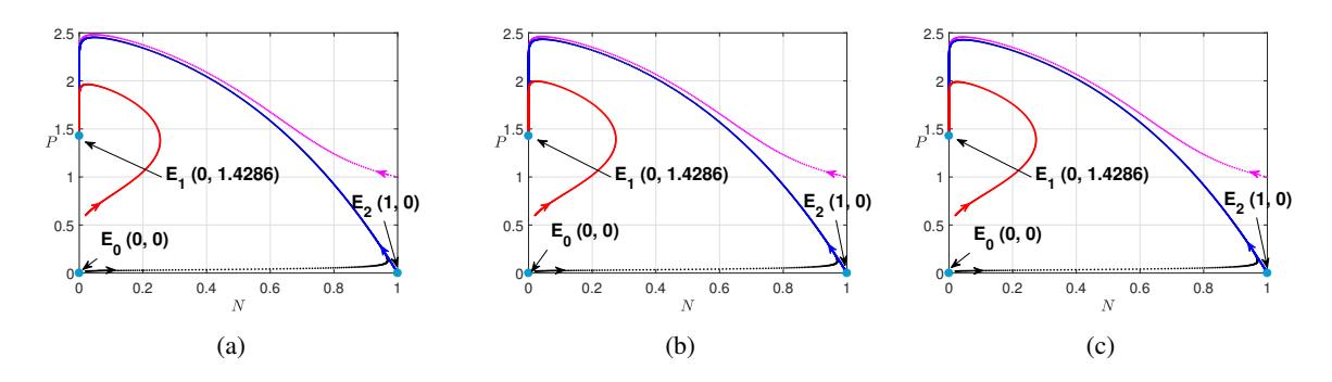
Figure 1: Phase portraits of simulation 1 with h = 0.05 using: (a) NSFD, (b) Euler, and (c) 4 th order Runge Kutta methods.
4.2. Simulation 2
To show the behavior of the solutions regarding the stability of predator extinction point, E2, the parameter values in Table 1 (Simulation 2) are chosen. With those parameter values, the stability conditons of E2(1, 0) are hold. This is in accordance with the results of the numerical simulation shown in Figure 3, with the step size used is h = 0.05. When the step size used is quite large as shown in Figure 4, i.e. h = 3.6, and by taking initial values near E2, the solutions of system (3) by Euler method is nonfeasible since they convergent to negative solutions, while the solutions by Runge Kutta leads to a periodic solutions of period two. Whereas, the stability of E2 is still consistent for NFSD scheme.
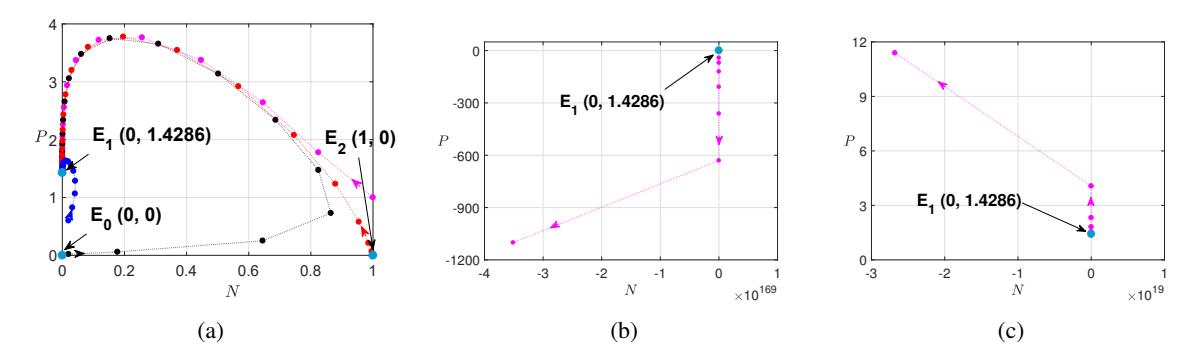
Figure 2: Phase portraits of simulation 1 with h=12 using: (a) NSFD, (b) Euler, and (c) \(4^{th}\) order Runge Kutta methods.
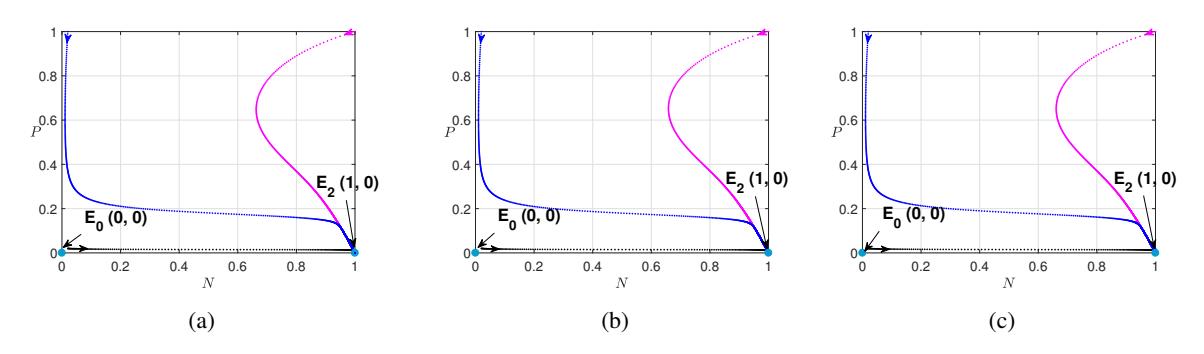
Figure 3: Phase portraits in simulation 2 with h=0.05 using: (a) NSFD, (b) Euler, and (c) \(4^{th}\) order Runge Kutta methods.
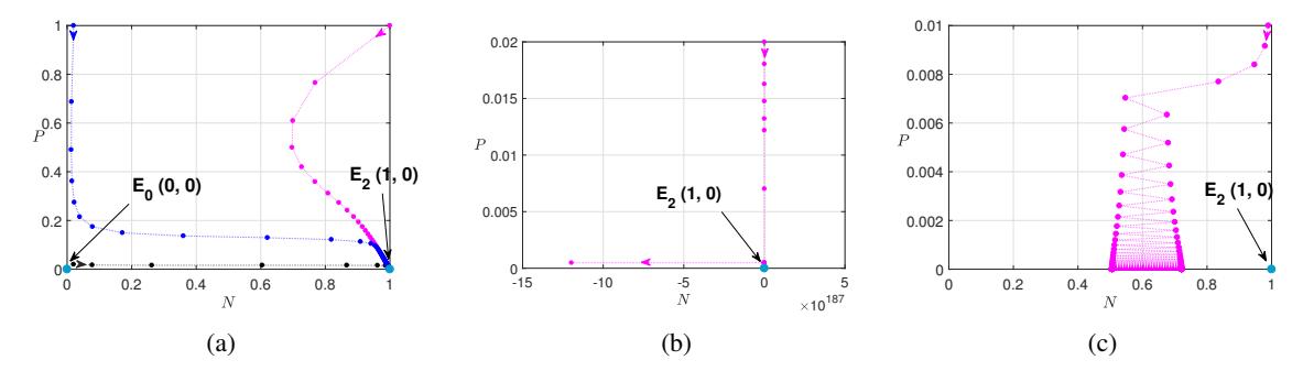
Figure 4: Phase portraits in simulation 2 with h=3.6 using: (a) NSFD, (b) Euler, and (c) \(4^{th}\) order Runge Kutta methods.
4.3. Simulation 3
With the parameter values in Table 1 (Simulation 3), the coexistence point exists, i.e. \(E_3(0.6026, 0.7174)\). For any values of h, all of the stability conditions of \(E_3\) in (14) are satisfied, as we can see in Figure 5. With a step size of h = 0.05 (see Figure 6), \(E_3\) is asymptotically stable for the NSFD, Euler, and \(4^{th}\) order
Runge Kutta methods. By increasing the step size value to h = 7.5 (see Figure 7), with initial values close to E3, the solutions of system (2) using Euler and 4 th order Runge Kutta methods lead to nonfeasible solutions (negative solutions), while the system with NSFD scheme is still consistent (see Figure 6). In Figure 7(c), the solution for predator goes down first then up.
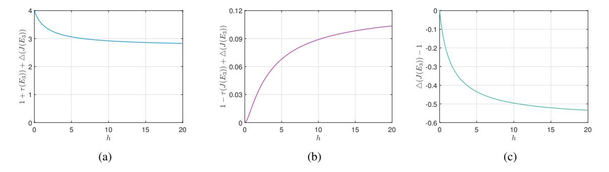
Figure 5: Graphics of (a) 1 + τ (J(E3)) + △(J(E3)), (b) 1 − τ (J(E3)) + △(J(E3)), and (c) △(J(E3)) − 1, in simulation 3.
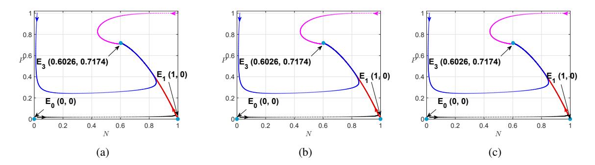
Figure 6: Phase portraits in simulation 3 with h = 0.05 using: (a) NSFD, (b) Euler, and (c) 4 th order Runge Kutta methods.
4.4. Simulation 4
By increasing the value of c1, as in Table 1 (Simulation 4), the coexistence point is E3(0.2631, 0.8299). The first two stability conditions of E3 in (14) are hold for any h, but the last condition isn't satisfied for 0 < h < 0.1006 (see Figure 8(c)) and is satisfied for all h ≥ 0.1006 (see Figure 8(d)). This is supported by the bifurcation diagram in Figure 9. For h < 0.1006, demonstrated particularly by h = 0.05 (Figure 10), the system convergent to a periodic solution. Meanwhile, for h > 0.1006 which is represented by h = 12 in Figure 11, the system convergent to coexistence point. In the continuous model in [18], with parameter values as in Table 1 (Simulation 4), the solutions do not converge to the coexistence point but to a limit cycle around it. In contrary, in the discrete model in this article, the solutions of system (3) can be stable to the coexistence point, by choosing the integration step-size larger than 0.1006.
Next, to compare the behavior of the system with the NSFD, Euler, and 4 th order Runge Kutta schemes, we choose h = 0.05 in simulation illustrated by Figure 12. While, in Figure 13 we choose h = 12. We can see that in Figure 12, the solutions of the three schemes convergent to a limit cycle around E3. In Figure 13 (h = 12), the solutions of NSFD scheme convergent to E3, whereas the two other schemes with initial value close to E3 convergent to nonfeasible (negative) solutions. In the results obtained in [18], the stability
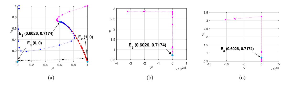
Figure 7: Phase portraits in simulation 3 with h = 7.5 using: (a) NSFD, (b) Euler, and (c) 4 th order Runge Kutta methods.
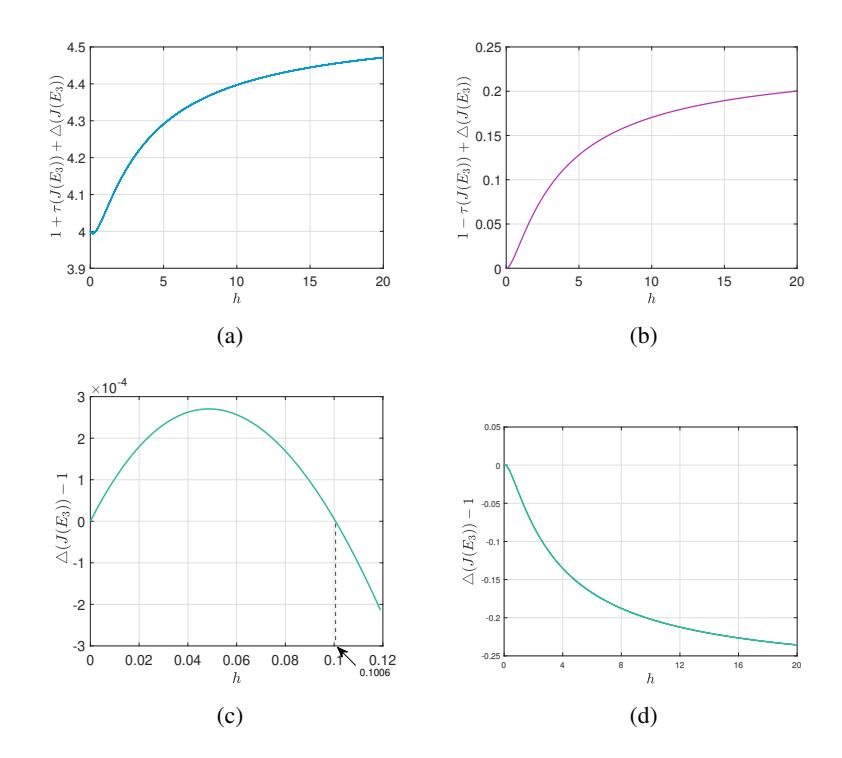
Figure 8: Graphics of (a) 1 + τ (J(E3)) + △(J(E3)), (b) 1 − τ (J(E3)) + △(J(E3)), (c) △(J(E3)) − 1 (for relative small h), and (d) △(J(E3)) − 1 (for 0 < h ≤ 20), in simulation 4.
of E3 is the same as the results in Figure 12. Thus, in this case, the stability properties of the NSFD system are only consistent with the continuous system for very small values of h. However, the advantage of NFSD here is that it keeps the solution positive, unlike the Euler and 4 th-order Runge-Kutta schemes which make the solutions turn to negative for large h values.
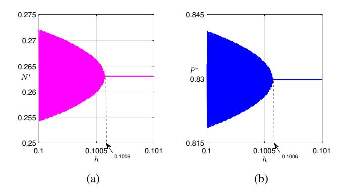
Figure 9: Diagram bifurcation in simulation 4 with h as bifurcation parameter: (a) h − N∗ , (b) h − P ∗ .
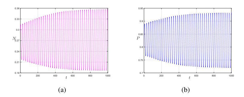
Figure 10: Solution of N and P in simulation 4 with h = 0.05: (a) t − N, (b) t − P.
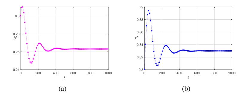
Figure 11: Solution of N and P in simulation 4 with h = 12: (a) t − N, (b) t − P.
5. CONCLUSION
In this paper, a discrete system of predator-prey model involving cannibalism and refuge in predator had been developed using Nonstandard Finite Difference (NFSD) scheme. Based on the analysis results, the system has four equilibrium points, i.e the origin, the prey extinction point, the predator extinction point, and the coexistence point which have exactly the same form and existence conditions as the ones in the continuous system. Furthermore, the local stability conditions for the first three equilibrium points have been
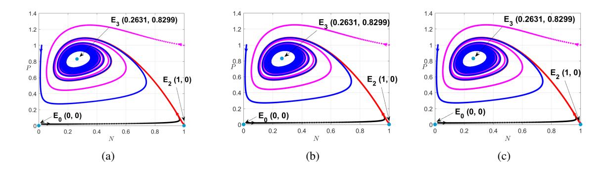
Figure 12: Phase portraits in simulation 4 with h = 0.05 using: (a) NSFD, (b) Euler, and (c) \(4^{th}\) order Runge Kutta methods.
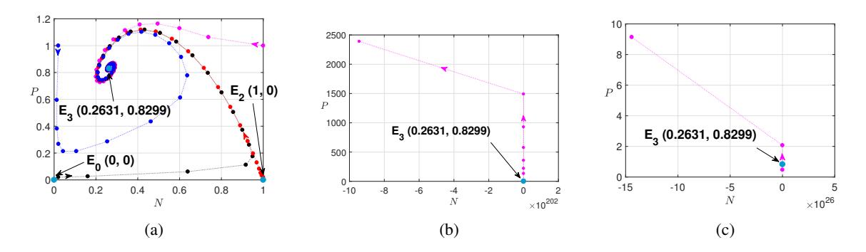
Figure 13: Phase portraits in simulation 4 with h = 12 using: (a) NSFD, (b) Euler, and (c) \(4^{th}\) order Runge Kutta methods.
shown to be exactly the same as those in the continuous system. Meanwhile, there are differences in the coexistence point's stability conditions. In the discrete system using an NSFD scheme the stability depends on the integration time step size, which does not occur in the continuous system. This is confirmed in numerical simulations which show that in some cases, the stability of the coexistence point is only consistent with the one in continuous system at a relative small step size, and inconsistent for step size that exceeds the threshold. Nonetheless, unlike the Euler and \(4^{th}\) order Runge-Kutta schemes, the NSFD scheme allows us to be more flexible in choosing the integration time stepsize for the solution to converge to a feasible point.
ACKNOWLEDGEMENT
This research is supported by Faculty of Mathematics and Natural Sciences (FMIPA) via Public Funds DPA (Dokumen Pelaksanaan Anggaran) Perguruan Tinggi Berbadan Hukum (PTNBH) University of Brawijaya and is based on FMIPA Professor Grant Contract No. 3084.19/UN10.F09/PN/2022.