

1. INTRODUCTION
Malaria is a disease caused by the parasite Plasmodium, transmitted by the bite of the female Anopheles mosquito which infected with the parasite Plasmodium. In general, five species of Plasmodium that can cause malaria, namely Plasmodium falciparum, Plasmodium vivax, Plasmodium malariae, Plasmodium ovale, and Plasmodium knowlesi. Of the five species, Plasmodium falciparum and Plasmodium vivax are the biggest causes of malaria in the world [1]. Based on data from the World Health Organization (WHO), malaria caused 405,000 cases of death out of a total 228 million in 2018. WHO also reported that the total funding for malaria control was estimated at 2.7 billion USD.
In regions of high malaria transmission, humans can be exposed to several hundred infected mosquitoes per year [2], which highly possibly bring several types of Plasmodium, such as P. Vivax and P. Falciparum. Many theories have been introduced to describe how superinfection in malaria occurs [3], [4]. They stated that superinfection occurs when single individuals human host more than one Plasmodium species, which might occur from consecutive bites or originated by a single bite of a mosquito who has multiple Plasmodium [5]. Nevertheless, it is well established that superinfection occurs in areas that have a high endemicity of malaria [6], wich suggesting that superinfection originates from consecutive infectious bites. In Indonesia, around 80% of the district/city is still categorized as malaria-endemic, and about 45% of the population lives in an area at risk of contracting malaria. This allows for superinfection in several malaria-endemic regions, including the Provinces of Maluku, North Maluku, Papua, West Papua, North Sumatra (Nias and Nias Selatan districts), and NTT [7]. This indicates that malaria superinfection is possible in Indonesia because it is a malaria-endemic area, and there are more than one species of Plasmodium in Indonesia.
*Corresponding author
One of malaria control strategy can be done by treatment for infected humans. Artemisinin-based Combination Therapies (ACT) is the best anti-malaria drug available nowadays. Artemisinin has the potential to reduce the level of resistance Plasmodium to appear and transmit in the human body [8]. Also, controlling malaria is not only done through treatment for infected humans, but also control of mosquitoes by fumigation. Fumigation is a method of controlling mosquitoes in which pesticide gas or steam is released to the air or injected to the ground to kill or eliminate mosquitoes. The benefit of fumigation is that it can reduce mosquito populations and reduce the intensity of malaria transmission by eliminating mosquitoes which are resting and breeding.
One way to study phenomena in the real world is by forming mathematical models [9]. Besides, mathematical modeling can help develop a scientific understanding of real-world problems, study the impact of each component, and make predictions behavior of the system. The superinfection problem described earlier can be compared with the SIR (host) – SI (vector) epidemic model. Furthermore, several studies have discussed the modeling of malaria, including the effect of anti-malaria resistant drugs [10], [11], effect of reinfection, relapse and/or recurrent [12], [13], [14], [15], [16], effect of bias mosquito preferences on blood resources [17], [18], [19], [20], superinfection phenomena [21], [22], model with coinfection with other diseases [23], [24], model with interventions [25], [26], [27], [28], [29], and many more.
Based on the background that has been explained, this research will discuss the formation of mathematical models regarding malaria superinfection transmission with medical treatment and fumigation interventions. Unlike the previous study conducted by Cai et al. [21], our article focuses on incorporating two distinct plasmodium strains into our proposed model. This approach is similar to our previous study discussed in [22]. However, there is a difference compared to [22] as we now consider an essential intervention factor in our model, specifically medical treatment and fumigation. Both of these interventions are widely practiced in many endemic areas to combat malaria. Additionally, we simplify our model using the Quassi Steady State Approximation (QSSA) by assuming that the mosquito population has already reached its equilibrium state. The question that will be addressed are: What is the mechanism of superinfection between Plasmodium Falciparum and Plasmodium Vivax? Can they coexist at the same time in the human population? How robust is our proposed model to the change of parameter value? Can the policymaker rely on fumigation and treatment to eradicate superinfection in the population? This paper seeks to answer the aforementioned question by the use of a mathematical model considering fumigation and treatment among superinfection phenomena.
Rest of the paper organized as follows. In Sec. 2, the mathematical model will be constructed and followed with a discussion on the positiveness and boundedness of the model solution. Mathematical analysis regarding the equilibrium points, control reproduction numbers, and invasion reproduction numbers given in Sec.3. Sensitivity analysis of all reproduction numbers and local sensitivity of the model are given in Sec. 4 followed with some examples of autonomous simulation in Sec. 5. Some conclusions given in the last section.
2. MODEL CONSTRUCTION
The first step in establishing a mathematical model of malaria superinfection transmission is divided the human population into four groups (susceptible, humans infected with Plasmodium falciparum, humans infected with Plasmodium vivax, and humans recovered from the infection) and then we divide mosquito population into three groups (susceptible, mosquitoes infected with Plasmodium falciparum, and mosquitoes infected with Plasmodium vivax). The transmission diagram of the model is shown in Figure 1.
If the transmission diagram is formed into the equation system, a model of malaria superinfection transmission is formed in the system (1). Variable S is a subpopulation of healthy people who are susceptible to infection, I1 is a subpopulation of humans infected with Plasmodium falciparum, I2 is a subpopulation of humans infected with Plasmodium vivax, R is a subpopulation of people who recovered from an infection, U is a subpopulation of healthy mosquitoes which are susceptible to infection, V1 is a subpopulation of mosquitoes infected with Plasmodium falciparum, and V2 is a subpopulation of mosquitoes infected with Plasmodium vivax.
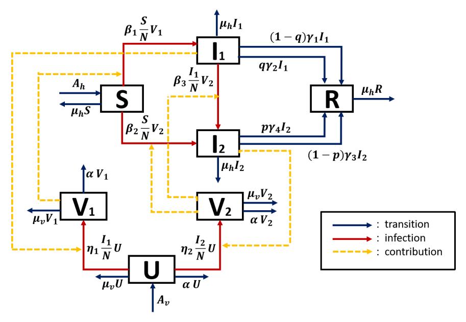
Figure 1: Transmission Diagram for Malaria Supreinfection with Medical Treatment and Fumigation. The blue and red lines represent the transition and infection processes, respectively. On the other hand, the yellow line represents the contribution of each variable to the infection process.
\[\frac{dS}{dt} = A_h - \beta_1 \frac{S}{N} V_1 - \beta_2 \frac{S}{N} V_2 - \mu_h S,\] (1a) \[\frac{dI_1}{dt} = \beta_1 \frac{S}{N} V_1 - \beta_3 \frac{I_1}{N} V_2 - (1 - q) \gamma_1 I_1 - q \gamma_2 I_1 - \mu_h I_1,\] (1b) \[\frac{dI_2}{dt} = \beta_2 \frac{S}{N} V_2 + \beta_3 \frac{I_1}{N} V_2 - (1 - p) \gamma_3 I_2 - p \gamma_4 I_2 - \mu_h I_2,\] (1c)
\[\frac{dI_1}{dt} = \beta_1 \frac{S}{N} V_1 - \beta_3 \frac{I_1}{N} V_2 - (1 - q) \gamma_1 I_1 - q \gamma_2 I_1 - \mu_h I_1, \tag{1b}\]
\[\frac{dI_2}{dt} = \beta_2 \frac{S}{N} V_2 + \beta_3 \frac{I_1}{N} V_2 - (1 - p) \gamma_3 I_2 - p \gamma_4 I_2 - \mu_h I_2, \tag{1c}\]
\[\frac{dR}{dt} = (1 - q)\gamma_1 I_1 + q\gamma_2 I_1 + (1 - p)\gamma_3 I_2 + p\gamma_4 I_2 - \mu_h R,\tag{1d}\]
\[\frac{dU}{dt} = A_v - \eta_1 \frac{I_1}{N} U - \eta_2 \frac{I_2}{N} U - \mu_v U - \alpha U, \tag{1e}\]
\[\frac{dR}{dt} = (1 - q)\gamma_1 I_1 + q\gamma_2 I_1 + (1 - p)\gamma_3 I_2 + p\gamma_4 I_2 - \mu_h R, \tag{1d}\] \[\frac{dU}{dt} = A_v - \eta_1 \frac{I_1}{N} U - \eta_2 \frac{I_2}{N} U - \mu_v U - \alpha U, \tag{1e}\] \[\frac{dV_1}{dt} = \eta_1 \frac{I_1}{N} U - \mu_v V_1 - \alpha V_1, \tag{1f}\] \[\frac{dV_2}{dt} = \eta_2 \frac{I_2}{N} U - \mu_v V_2 - \alpha V_2, \tag{1g}\]
\[\frac{dV_2}{dt} = \eta_2 \frac{I_2}{N} U - \mu_v V_2 - \alpha V_2,\tag{1g}\]
Susceptible human and mosquito subpopulations can increase due to births of \(A_h\) and \(A_v\), respectively. Each human and mosquito subpopulation can be reduced due to natural mortality at a rate of \(\mu_h\) and \(\mu_v\), respectively. There is an additional deaths in mosquito population due to furnigation at a rate of \(\alpha\). Susceptible humans can get infected by malaria only due to contact with infected mosquitoes with its specific rate depending on the type of the Plasmodium. The rate of infection in the human population due to Plasmodium falciparum and Plasmodium vivax is given by \(\beta_1\) and \(\beta_2\), respectively. On the other hand, The rate of infection in mosquitoes population due to Plasmodium falciparum and Plasmodium vivax is given by \(\eta_1\) and \(\eta_2\), respectively. Our model accommodates the superinfection phenomena, where Plasmodium vivax can dominate Plasmodium falciparum. Therefore, if \(I_1\) gets a successful infection by \(V_2\) with a rate of \(\beta_3\), they will become infected by Plasmodium vivax. Due to the short lifetime period of the mosquito population, we assume no superinfection phenomena in the mosquito population. Humans who have been infected could be recover from infection, both with treatment or not. The proportion of humans recovering from infections \(Plasmodium\ falciparum\) without treatment is (1-q) with a recovery rate of \(\gamma_1\) and the proportion (1-p) is for humans recovering from infections \(Plasmodium\ vivax\) without treatment with a recovery rate of \(\gamma_3\). Furthermore, the proportion of people who have recovered from infection \(Plasmodium\ falciparum\) with treatment is q at the recovery rate of \(\gamma_2\) and the proportion p is for humans recovering from infections \(Plasmodium\ vivax\) with treatment at the recovery rate of \(\gamma_4\). The total human population \((N(t) = S(t) + I_1(t) + I_2(t) + R(t))\) in this model is assumed to be constant and closed.
2.1. Positiveness
To show that the malaria superinfection model is epidemiologically meaningful, we will prove that all the solutions of model (1) are positive for all time t > 0.
Theorem 2.1. Given the initial condition of the model in system (1), where \(S(0) \ge 0\), \(I_1(0) \ge 0\), \(I_2(0) \ge 0\), \(I_2(0) \ge 0\), \(I_2(0) \ge 0\), \(I_2(0) \ge 0\), \(I_2(0) \ge 0\), \(I_2(0) \ge 0\), \(I_2(0) \ge 0\), \(I_2(0) \ge 0\), \(I_2(0) \ge 0\), then the solution \(I_2(0) \ge 0\), \(I_2(0) \ge 0\), \(I_2(0) \ge 0\), \(I_2(0) \ge 0\), then the solution \(I_2(0) \ge 0\), \(I_2(0) \ge 0\), \(I_2(0) \ge 0\), \(I_2(0) \ge 0\), then the solution \(I_2(0) \ge 0\), \(I_2(0) \ge 0\), \(I_2(0) \ge 0\), \(I_2(0) \ge 0\), then the solution \(I_2(0) \ge 0\), \(I_2(0) \ge 0\), \(I_2(0) \ge 0\), \(I_2(0) \ge 0\), then the solution \(I_2(0) \ge 0\), \(I_2(0) \ge 0\), \(I_2(0) \ge 0\), \(I_2(0) \ge 0\), \(I_2(0) \ge 0\), \(I_2(0) \ge 0\), \(I_2(0) \ge 0\), \(I_2(0) \ge 0\), \(I_2(0) \ge 0\), \(I_2(0) \ge 0\), \(I_2(0) \ge 0\), \(I_2(0) \ge 0\), \(I_2(0) \ge 0\), \(I_2(0) \ge 0\), \(I_2(0) \ge 0\), \(I_2(0) \ge 0\), \(I_2(0) \ge 0\), \(I_2(0) \ge 0\), \(I_2(0) \ge 0\), \(I_2(0) \ge 0\), \(I_2(0) \ge 0\), \(I_2(0) \ge 0\), \(I_2(0) \ge 0\), \(I_2(0) \ge 0\), \(I_2(0) \ge 0\), \(I_2(0) \ge 0\), \(I_2(0) \ge 0\), \(I_2(0) \ge 0\), \(I_2(0) \ge 0\), \(I_2(0) \ge 0\), \(I_2(0) \ge 0\), \(I_2(0) \ge 0\), \(I_2(0) \ge 0\), \(I_2(0) \ge 0\), \(I_2(0) \ge 0\), \(I_2(0) \ge 0\), \(I_2(0) \ge 0\), \(I_2(0) \ge 0\), \(I_2(0) \ge 0\), \(I_2(0) \ge 0\), \(I_2(0) \ge 0\), \(I_2(0) \ge 0\), \(I_2(0) \ge 0\), \(I_2(0) \ge 0\), \(I_2(0) \ge 0\), \(I_2(0) \ge 0\), \(I_2(0) \ge 0\), \(I_2(0) \ge 0\), \(I_2(0) \ge 0\), \(I_2(0) \ge 0\), \(I_2(0) \ge 0\), \(I_2(0) \ge 0\), \(I_2(0) \ge 0\), \(I_2(0) \ge 0\), \(I_2(0) \ge 0\), \(I_2(0) \ge 0\), \(I_2(0) \ge 0\), \(I_2(0) \ge 0\), \(I_2(0) \ge 0\), \(I_2(0) \ge 0\), \(I_2(0) \ge 0\), \(I_2(0) \ge 0\), \(I_2(0) \ge 0\), \(I_2(0) \ge 0\), \(I_2(0) \ge 0\), \(I_2(0) \ge 0\), \(I_2(0) \ge 0\), \(I_2(0) \ge 0\), \(I_2(0) \ge 0\), \(I_2(0) \ge 0\), \(I_2(0) \ge 0\), \(I_2(0) \ge 0\), \(I_2(0) \ge 0\), \(I_2(0) \ge 0\), \(I_2(0) \ge 0\), \(I_2(0) \ge 0\), \(I_2(0) \ge 0\), \(I_2(0) \ge 0\), \(I_2(0) \ge 0\), \(I_2(0) \ge 0\), \(I_2(0) \ge 0\), \(I_2(0) \ge 0\), \(I_2(0) \ge 0\), \(I_2(0) \ge 0\), \(I_2(0) \ge 0\), \(I_2(0) \ge 0\), \(I_2(0) \ge 0\), \(I_2(0) \ge 0\), \(I_2(0) \ge 0\), \(I_2(0) \ge 0\), \(I_2(0) \ge 0\), \(I_2(0) \ge 0\), \(I_2(0) \ge 0\), \(I_2(0) \ge 0\), \(I_2(0) \ge 0\), \(I_2(0) \ge 0\), \(I_2(0) \ge 0\), \(I_2(0) \ge 0\), \(I_2(0) \ge 0\), \(I_2(0) \ge 0\), \(I_2(0) \ge 0\), \(I_2(0) \ge 0\), \(I_2(0) \ge 0\), \(I_2(0) \ge 0\), \(I_2(0) \ge 0\), \(I_2(0) \ge 0\), \(I_2(0) \ge 0\), \(I_2\)
Proof: From system (1), we have
\[\begin{split} \frac{dS}{dt}(S=0,I_1\geq 0,I_2\geq 0,R\geq 0,U>0,V_1\geq 0,V_2\geq 0) &=& A_h>0,\\ \frac{dI_1}{dt}(S>0,I_1=0,I_2\geq 0,R\geq 0,U>0,V_1\geq 0,V_2\geq 0) &=& \beta_1\frac{S}{N}V_1\geq 0,\\ \frac{dI_2}{dt}(S>0,I_1\geq 0,I_2=0,R\geq 0,U>0,V_1\geq 0,V_2\geq 0) &=& \beta_2\frac{S}{N}V_2+\beta_3\frac{I_1}{N}V_2\geq 0,\\ \frac{dR}{dt}(S>0,I_1\geq 0,I_2\geq 0,R=0,U>0,V_1\geq 0,V_2\geq 0) &=& (1-q)\gamma_1I_1+q\gamma_2I_1+(1-p)\gamma_3I_2\\ &&+p\gamma_4I_2\geq 0,\\ \frac{dU}{dt}(S>0,I_1\geq 0,I_2\geq 0,R\geq 0,U=0,V_1\geq 0,V_2\geq 0) &=& A_v>0,\\ \frac{dV_1}{dt}(S>0,I_1\geq 0,I_2\geq 0,R\geq 0,U>0,V_1=0,V_2\geq 0) &=& \eta_1\frac{I_1}{N}U\geq 0,\\ \frac{dV_1}{dt}(S>0,I_1\geq 0,I_2\geq 0,R\geq 0,U>0,V_1\geq 0,V_2=0) &=& \eta_2\frac{I_2}{N}U\geq 0. \end{split}\]
From above calculation, all the rates in the boundary planes are non-negative in the boundary of \(\mathbb{R}^7_+\). Hence, we can conclude that as long as the initial conditions are non-negative, then all vector field direction will be inward from the boundary planes. Hence, all the solutions remain in the positive region only. Here the proof is completed.
2.2. Boundedness
Theorem 2.2. In the system (1), each human subpopulations \((S(t), I_1(t), I_2(t), R(t))\) and each mosquito subpopulations \((U(t), V_1(t), V_2(t))\) are bounded.
Proof: By adding up the total number of human subpopulations and mosquito subpopulations from the equation system (1), we obtained \(\frac{dN}{dt} = A_h - \mu_h N\) and \(\frac{dM}{dt} = A_v - (\mu_v + \alpha)M\). Since we assume that number of recruitment rate is always the same with total of death, and no migration consider in the model, then we have that \(\frac{dN}{dt} = 0\), which implies that N is a constant. Based on Theorem 2.1, all human population is always positive for all time t > 0. Hence, we have that \(S(t), I_1(t), I_2(t)\), and R(t) are bounded below by 0 and above by \(\frac{A_h}{\mu_h}\).
Boundedness of mosquito subpopulations will be proof by integration factor.
\[\frac{dM}{dt} = A_v - (\mu_v + \alpha)M,\] \[\iff \frac{dM}{dt} + (\mu_v + \alpha)M = A_v,\] \[\iff \frac{d}{dt} \left[ Me^{\mu_v t + \alpha t} \right] = A_v e^{\mu_v t + \alpha t},\] \[\iff M(t_i)e^{\mu_v t_i + \alpha t_i} - M(0) = A_v \int_0^{t_i} e^{\mu_v t + \alpha t} dt,\] \[\iff M(t_i) = \frac{A_v}{\mu_v + \alpha} + \frac{c}{e^{\mu_v t_i + \alpha t_i}}.\]
For \(t_i \to \infty\) we obtained
\[\lim_{t_i \to \infty} M(t) \le \frac{A_v}{(\mu_v + \alpha)}.\]
So, mosquito subpopulations are bounded by \(M(t) \leq \frac{A_v}{(\mu_v + \alpha)}\). Its corollary of \(M = U + V_1 + V_2\) and \(U(t), V_1(t), V_2(t)\), are always positive, it means \(0 \leq U(t) \leq \frac{A_v}{(\mu_v + \alpha)}, 0 \leq V_1(t) \leq \frac{A_v}{(\mu_v + \alpha)}\), and \(0 \leq V_2(t) \leq \frac{A_v}{(\mu_v + \alpha)}\). Hence, \(U(t), V_1(t)\), and \(V_2(t)\) are bounded in \(\left[0, \frac{A_v}{\mu_v + \alpha}\right]\).
2.3. Invariant Region
Based on Theorem 2.1 and Theorem 2.2, a positive invariant region can be created as a result of positiveness and boundedness solutions.
Corollary 2.2.1. Region \(\Omega \in \mathbb{R}^7_+ \cup \mathbf{0}^7\) with \(\Omega = \Omega_n \times \Omega_m\) and
\[\Omega_n = \left\{ (S, I_1, I_2, R) \in \mathbb{R}_+^4 \cup \mathbf{0}^4 : S + I_1 + I_2 + R = \frac{A_h}{\mu_h} \right\}, \Omega_m = \left\{ (U, V_1, V_2) \in \mathbb{R}_+^3 \cup \mathbf{0}^3 : M(t) \le \frac{A_v}{(\mu_v + \alpha)} \right\},\] is positively invariant for the system (1) with initial conditions that are always non-negative in \(\mathbb{R}^7_+ \cup \mathbf{0}^7\).
3. MODEL ANALYSIS
3.1. Quasi-Steady State Approximation (QSSA)
QSSA can be used when there is a part of the system reacts much faster than the other, so it can be said that the system has a slow and fast dynamic. In our model, the mosquito has a very short lifetime period compared to humans. Mosquito lives only for 21 days, while a human can live up to 72 years old. Hence, it is clear that mosquitoes can reach the equilibrium much faster compared to humans. This fact implies that a mosquito has fast dynamics while a human has slow dynamics. Then, we can simplify the part that reacts faster on the system to the slower part reducing the number of variables [30]. The process of implementing QSSA to our mosquito population is as follows. Solving \(\frac{dU}{dt} = 0\), \(\frac{dV_1}{dt} = 0\) and \(\frac{dV_2}{dt} = 0\) respect to \(U, V_1\) and \(V_2\), we have:
\[U^* = \frac{A_v N}{N\alpha + N\mu_v + \eta_1 I_1 + \eta_2 I_2}, V_1^* = \frac{A_v \eta_1 I_1}{(\alpha + \mu_v)(N\alpha + N\mu_v + \eta_1 I_1 + \eta_2 I_2)},\]\[V_2^* = \frac{A_v \eta_2 I_2}{(\alpha + \mu_v)(N\alpha + N\mu_v + \eta_1 I_1 + \eta_2 I_2)}.\]
Next, we substitute \(U_1^*, V_1^*, V_2^*\) and \(R = N - (S + I_1 + I_2)\), into \(\frac{dS}{dt}, \frac{dI_1}{dt}, \frac{dI_2}{dt}\), we have
\[\frac{dS}{dt} = A_h - \frac{\beta_1 \eta_1 A_v S I_1}{C_1} - \frac{\beta_2 \eta_2 A_v S I_2}{C_1} - \mu_h S, \tag{2a}\]
\[\frac{dI_1}{dt} = \frac{\beta_1 \eta_1 A_v S I_1}{C_1} - \frac{\beta_3 \eta_2 A_v I_1 I_2}{C_1} - (1 - q) \gamma_1 I_1 - q \gamma_2 I_1 - \mu_h I_1, \tag{2b}\]
\[\frac{dI_2}{dt} = \frac{\beta_1 \eta_1 A_v S I_1}{C_1} + \frac{\beta_3 \eta_2 A_v I_1 I_2}{C_1} - (1 - p)\gamma_3 I_2 - p\gamma_4 I_2 - \mu_h I_2, \tag{2c}\] where \(C_1 = N(\alpha + \mu_v)(N\alpha + N\mu_v + \eta_1 I_1 + \eta_2 I_2)\). System (2) is the model that we will analyze in the following section, instead of the original model in (1). Note that simplification using QSSA in this research can reduce the dimensions of the system that originally had a dimension of 7 to a dimension of 3. This is expected to simplify the model analysis.
3.2. Disease Free Equilibrium and The Control Reproduction Number
Disease-free equilibrium point \((\mathcal{E}_0)\) is a condition where the disease has appeared in a population, but then will be disappear over time. The DFE point, \(\mathcal{E}_0=(S,0,0)\), is obtained from the system (2) substituted with \(\frac{dS}{dt}=0\), \(I_1=0\), and \(I_2=0\) so the following results are obtained
\[A_h - \mu_h S = 0 \Longleftrightarrow S = \frac{A_h}{\mu_h}.\]
So, we obtained the disease-free equilibrium
\[\mathcal{E}_0 = (S, 0, 0) = \left(\frac{A_h}{\mu_h}, 0, 0\right),\]
will always exist or have biological meaning without any conditions.
Theorem 3.1. Disease-free equilibrium point \(\mathcal{E}_0\) from the system (2) will always exist without any conditions, where \(\mathcal{E}_0 = \left(\frac{A_h}{\mu_h}, 0, 0\right)\).
1). The Control Reproduction Number
Furthermore, we calculate the control reproduction number \((\mathcal{R}_0)\) using the next-generation matrix (NGM) [31]. The steps taken are as follows. The transmission \(\mathbf{T}\) and transition \(\mathbf{\Sigma}\) matrix of system (2) is given by
\[\mathbf{T} = \begin{bmatrix} \frac{A_h A_v \beta_1 \eta_1}{\mu_h N^2 (\alpha + \mu_v)^2} & 0 \\ 0 & \frac{A_h A_v \beta_2 \eta_2}{\mu_h N^2 (\alpha + \mu_v)^2} \end{bmatrix}, \quad \mathbf{\Sigma} = \begin{bmatrix} -(1-q)\gamma_1 - q\gamma_2 - \mu_h & 0 \\ 0 & -(1-p)\gamma_3 - p\gamma_4 - \mu_h \end{bmatrix}.\]
Hence, the next-generation matrix of system (2) is given by
\[\mathbf{K} = \mathbf{K} \mathbf{\Sigma}^{-1} = \mathbf{K} = \begin{bmatrix} \frac{A_h A_v \beta_1 \eta_1}{\mu_h N^2 (\alpha + \mu_v)^2 ((1 - q) \gamma_1 + q \gamma_2 + \mu_h)} & 0\\ 0 & \frac{A_h A_v \beta_2 \eta_2}{\mu_h N^2 (\alpha + \mu_v)^2 ((1 - p) \gamma_3 + p \gamma_4 + \mu_h)} \end{bmatrix}.\](3)
Hence, the control reproduction number of system (2) as a spectral radius of K is given by
\[\mathcal{R}_0 = \max\left\{\mathcal{R}_{01}, \mathcal{R}_{02}\right\},\tag{4}\]
where
\[\mathcal{R}_{01} = \frac{A_h A_v \beta_1 \eta_1}{\mu_h N^2 (\alpha + \mu_v)^2 ((1 - q)\gamma_1 + q\gamma_2 + \mu_h)},\] \[\mathcal{R}_{02} = \frac{A_h A_v \beta_2 \eta_2}{\mu_h N^2 (\alpha + \mu_v)^2 ((1 - p)\gamma_3 + p\gamma_4 + \mu_h)}.\]
Note that, \(\mathcal{R}_{01}\) is the control reproduction number of the system for infection with Plasmodium falciparum, while \(\mathcal{R}_{02}\) is the control reproduction number of the system for infection with Plasmodium vivax.
Theorem 3.2. The control reproduction number from the system (2) is \(\mathcal{R}_0 = \max \{\mathcal{R}_{01}, \mathcal{R}_{02}\}\).
In many epidemiological models such as in malaria [17], [18], [27] or in other diseases [32], [33], [34], [35], [36], [37], it is common to see that the disease will persist whenever the control reproduction number is less than unity, and exist otherwise. In the next analysis, we will show that malaria will persist from the community using our proposed model whenever both the basic reproduction number in 4 is less than unity. The local stability of \(\mathcal{E}_0\) is summarized in the following theorem.
Theorem 3.3. The disease-free equilibrium \((\mathcal{E}_0)\) of the system (2) is locally asymptotically stable if \(\mathcal{R}_0 < 1\).
Proof: Linearize system (2) in \(\mathcal{E}_0\) gave us
\[J_{\mathcal{E}_0} = \begin{bmatrix} -\mu_h & -\frac{A_h A_v \beta_1 \eta_1}{\mu_h N^2 (\alpha + \mu_v)^2} & -\frac{A_h A_v \beta_2 \eta_2}{\mu_h N^2 (\alpha + \mu_v)^2} \\ 0 & -\frac{A_h A_v \beta_1 \eta_1}{\mu_h N^2 (\alpha + \mu_v)^2} - (1 - q) \gamma_1 - q \gamma_2 - \mu_h & 0 \\ 0 & 0 & -\frac{A_h A_v \beta_2 \eta_2}{\mu_h N^2 (\alpha + \mu_v)^2} - (1 - p) \gamma_3 + p \gamma_4 - \mu_h \end{bmatrix}.\]
The polynomial characteristic of \(J_{\mathcal{E}_0}\) is
\[(\lambda + \mu_h) \left( \lambda - \frac{A_h A_v \beta_1 \eta_1}{\mu_h N^2 (\alpha + \mu_v)^2} + (1 - q) \gamma_1 + q \gamma_2 + \mu_h \right) \left( \lambda - \frac{A_h A_v \beta_2 \eta_2}{\mu_h N^2 (\alpha + \mu_v)^2} + (1 - p) \gamma_3 + p \gamma_4 + \mu_h \right) = 0.\]
Hence, the eigenvalues are
\[\lambda_1 = -\mu_h, \ \lambda_2 = -((1-q)\gamma_1 + q\gamma_2 + \mu_h)(1 - \mathcal{R}_{01}), \ \lambda_3 = -((1-p)\gamma_3 + p\gamma_4 + \mu_h)(1 - \mathcal{R}_{02})\]
It is easy to see that all eigenvalues \(\lambda\) will be negative if \(\mathcal{R}_{01} < 1\), \(\mathcal{R}_{02} < 1 \iff \mathcal{R}_0 < 1\).
2). Some Notes on The Control and Basic Reproduction Numbers
From the expression of the control reproduction number in (4), the basic reproduction number of system (2) is given when all controls are 0 (\(p = 0, q = 0, \alpha = 0\)). Hence, the basic reproduction number of system (2) is given by
\[\mathcal{R}_{0}^{*} = \max\left\{\mathcal{R}_{01}^{*}, \mathcal{R}_{02}^{*}\right\} = \max\left\{\frac{A_{h}A_{v}\beta_{1}\eta_{1}}{\mu_{h}N^{2}\mu_{v}^{2}(\gamma_{1} + \gamma_{2} + \mu_{h})}, \frac{A_{h}A_{v}\beta_{2}\eta_{2}}{\mu_{h}N^{2}\mu_{v}^{2}(\gamma_{3} + \gamma_{4} + \mu_{h})}\right\}. \tag{5}\]
It can be seen that \(\mathcal{R}_{01} < \mathcal{R}_{01}^*\) and \(\mathcal{R}_{02} < \mathcal{R}_{02}^*\). Hence, we can verify that implementation of treatment and fumigation can reduce the reproduction number. Furthermore, the expression of \(\mathcal{R}_{01}\) can be rewritten as follows
\[\mathcal{R}_{01} = \frac{M}{N} \times \frac{\beta_1}{(1-q)\gamma_1 + q\gamma_2 + \mu_h} \times \frac{\eta_1}{\alpha + \mu_v}\] Ratio of human and mosquito New infection in human New infection in mosquito
\(\mathcal{R}_{02}\) can be expresses in a similar way as in (6). From the expression above, each control contribute in a different term of \(\mathcal{R}_{01}\). Controlling the spread of malaria do not always need both controls implemented together. There is a level of minimum implementation for each controls such that \(\mathcal{R}_{0i}\) for i=1,2 can be reduced.
3.3. Endemic Equilibrium
Endemic equilibrium is a condition where the disease epidemic in the population. Endemic equilibrium is obtained from the system (2) substituted with \(\frac{dS}{dt}=0\), \(\frac{dI_1}{dt}=0\), and \(\frac{dI_2}{dt}=0\). By solving it, we get three endemic equilibrium points.
1). Plasmodium Falciparum-Only
Endemic equilibrium point for Plasmodium falciparum-only, denoted by \(\mathcal{E}_1\), is given by
\[S^* = \frac{N^2 \left( (1 - q)\gamma_1 + q\gamma_2 + \mu_h \right) + NA_h \eta_1(\alpha + \mu_v)}{\eta_1 \left( N\mu_h(\alpha + \mu_v) + A_v \beta_1 \right)}, I_1^* = \frac{N^2 \mu_h(\alpha + \mu_v) (\mathcal{R}_{01} - 1)}{\eta_1 \left( N\mu_h(\alpha + \mu_v) + A_v \beta_1 \right)}, I_2^* = 0.\]
The existence and local stability criteria of \(\mathcal{E}_1\) is summarized in the following theorem.
Theorem 3.4. Endemic equilibrium point \(\mathcal{E}_1\) exist if \(\mathcal{R}_{01} > 1\) and locally asymptotically stable if the invasion reproduction number of P. Falciparum to P. Vivax given by
\[\mathcal{R}_{1}^{2} = \frac{N(\alpha + \mu_{v}) \left(N(\alpha + \mu_{v}) \left((1 - q)\gamma_{1} + q\gamma_{2} + \mu_{h}\right) + A_{h}\eta_{1}\right) \left((1 - p)\gamma_{3} + p\gamma_{4} + \mu_{h}\right) \left(\mathcal{R}_{01} - \mathcal{R}_{02}\right)}{A_{h}A_{v}\beta_{3}\eta_{2}(\mathcal{R}_{01} - 1)}\] is larger than unity.
Proof: It is clear that \(I_1^*\) will be positive or epidemiologically meaningful if \(\mathcal{R}_{01} > 1\). Furthermore, characteristic equation of Jacobian matrix of system (2) near \(\mathcal{E}_1\) can be written as follows
\[(a_1\lambda + a_0)(b_2\lambda^2 + b_1\lambda + b_0) = 0, (7)\] where
\[a_{1} = \beta_{1}\eta_{1}(\alpha + \mu_{v}) \left(N(\alpha + \mu_{v}) \left((1 - q)\gamma_{1} + q\gamma_{2} + \mu_{h}\right) + A_{h}\eta_{1}\right) > 0,\] \[a_{0} = N(\alpha + \mu_{v}) \left(N(\alpha + \mu_{v}) \left((1 - q)\gamma_{1} + q\gamma_{2} + \mu_{h}\right) + A_{h}\eta_{1}\right) \left((1 - p)\gamma_{3} + p\gamma_{4} + \mu_{h}\right) \left(\mathcal{R}_{01} - \mathcal{R}_{02}\right) - A_{h}A_{v}\beta_{3}\eta_{2}(\mathcal{R}_{01} - 1),\] \[b_{2} = \beta_{1}A_{v}(\alpha + \mu_{v}) \left(N(\alpha + \mu_{v}) \left((1 - q)\gamma_{1} + q\gamma_{2} + \mu_{h}\right) + A_{h}\eta_{1}\right) > 0,\] \[b_{1} = \mathcal{R}_{01} \left(N(\alpha + \mu_{v}) \left((1 - q)\gamma_{1} + q\gamma_{2} + 2\mu_{h}\right) + A_{v}\eta_{1}\right) - N(\alpha + \mu_{v}) \left((1 - q)\gamma_{1} + q\gamma_{2} + \mu_{h}\right),\] \[b_{0} = \mu_{h}(\alpha + \mu_{v})^{2} \left(N\mu_{h}(\alpha + \mu_{v})\right) \left((1 - q)\gamma_{1} + q\gamma_{2} + \mu_{h}\right)^{2} \left(\mathcal{R}_{01} - 1\right) > 0.\]
Therefore, all roots of equation (7) have a negative real part if and only if \(a_0 > 0\) and \(b_1 > 0\). To guarantee a positive value of \(a_0\), it should be
\[\mathcal{R}_{1}^{2} = \frac{N(\alpha + \mu_{v})\left(N(\alpha + \mu_{v})\left((1 - q)\gamma_{1} + q\gamma_{2} + \mu_{h}\right) + A_{h}\eta_{1}\right)\left((1 - p)\gamma_{3} + p\gamma_{4} + \mu_{h}\right)\left(\mathcal{R}_{01} - \mathcal{R}_{02}\right)}{A_{h}A_{v}\beta_{3}\eta_{2}(\mathcal{R}_{01} - 1)} > 1.\]
The positive value of \(b_1\) is a direct implication by \(-\frac{b_1}{b_2} < 0\) (the roots of the two-degree polynomial are negative if the sum is also negative). So, this completes the proof.
2). Plasmodium Vivax-Only
Endemic equilibrium point for Plasmodium vivax-only, denoted by \(\mathcal{E}_2\), is given by
\[S^{**} = \frac{N^2 \left( (1-p)\gamma_3 + p\gamma_4 + \mu_h \right) + NA_h \eta_2(\alpha + \mu_v)}{\eta_2 \left( N\mu_h(\alpha + \mu_v) + A_v \beta_2 \right)}, I_1^{**} = 0, I_2^{**} = \frac{N^2 \mu_h(\alpha + \mu_v)(\mathcal{R}_{02} - 1)}{\eta_2 \left( N\mu_h(\alpha + \mu_v) + A_v \beta_2 \right)}.\]
The existence and local stability criteria of \(\mathcal{E}_2\) is given in the following theorem.
Theorem 3.5. Endemic equilibrium point of \(\mathcal{E}_2\) from the system (2) exists if \(\mathcal{R}_{02} > 1\) and locally stable if the invasion reproduction number of P. Vivax to P. Falciparum
\[\mathcal{R}_{2}^{1} = \frac{A_{h}A_{v}\beta_{3}\eta_{2}(\mathcal{R}_{02} - 1)}{N(\alpha + \mu_{v})\left(N(\alpha + \mu_{v})\left((1 - p)\gamma_{3} + p\gamma_{4} + \mu_{h}\right) + A_{h}\eta_{2}\right)\left((1 - p)\gamma_{3} + p\gamma_{4} + \mu_{h}\right)\left(\mathcal{R}_{01} - \mathcal{R}_{02}\right)}\]
larger than unity.
Proof: It is clear that \(I_2^*\) will be positive or epidemiologically meaningful if \(\mathcal{R}_{02} > 1\). Furthermore, characteristic equation of Jacobian matrix of system (2) near \(\mathcal{E}_2\) can be written as follows
\[(c_1\lambda + c_0)(d_2\lambda^2 + d_1\lambda + d_0) = 0, (8)\]
where
\[c_{1} = \beta_{2}\eta_{2}(\alpha + \mu_{v}) \left( N(\alpha + \mu_{v}) \left( (1 - p)\gamma_{3} + p\gamma_{4} + \mu_{h} \right) + A_{h}\eta_{4} \right) > 0,\] \[c_{0} = A_{h}A_{v}\beta_{3}\eta_{2}(\mathcal{R}_{02} - 1) - N(\alpha + \mu_{v}) \left( N(\alpha + \mu_{v}) \left( (1 - p)\gamma_{3} + p\gamma_{4} + \mu_{h} \right) + A_{h}\eta_{2} \right)\] \[\left( (1 - p)\gamma_{3} + p\gamma_{4} + \mu_{h} \right) \left( \mathcal{R}_{01} - \mathcal{R}_{02} \right),\] \[d_{2} = \beta_{1}A_{v}(\alpha + \mu_{v}) \left( N(\alpha + \mu_{v}) \left( (1 - p)\gamma_{3} + p\gamma_{4} + \mu_{h} \right) + A_{h}\eta_{2} \right) > 0,\] \[d_{1} = \mathcal{R}_{02} \left( N(\alpha + \mu_{v}) \left( (1 - p)\gamma_{3} + p\gamma_{4} + 2\mu_{h} \right) + A_{v}\eta_{4} \right) - N(\alpha + \mu_{v}) \left( (1 - p)\gamma_{3} + p\gamma_{4} + \mu_{h} \right),\] \[d_{0} = \mu_{h}(\alpha + \mu_{v})^{2} \left( N\mu_{h}(\alpha + \mu_{v}) \right) \left( (1 - p)\gamma_{3} + p\gamma_{4} + \mu_{h} \right)^{2} \left( \mathcal{R}_{02} - 1 \right) > 0.\]
Therefore, all roots of equation (8) have a negative real part if and only if \(a_0 > 0\) and \(b_1 > 0\). To guarantee a positive value of \(a_0\), it should be
\[\mathcal{R}_{2}^{1} = \frac{A_{h}A_{v}\beta_{3}\eta_{2}(\mathcal{R}_{02} - 1)}{N(\alpha + \mu_{v})\left(N(\alpha + \mu_{v})\left((1 - p)\gamma_{3} + p\gamma_{4} + \mu_{h}\right) + A_{h}\eta_{2}\right)\left((1 - p)\gamma_{3} + p\gamma_{4} + \mu_{h}\right)\left(\mathcal{R}_{01} - \mathcal{R}_{02}\right)} > 1.\]
The ositive value of \(b_1\) is a direct implication by \(-\frac{b_1}{b_2} < 0\) (the roots of the two-degree polynomial are negative if the sum is also negative). So, this completes the proof.
3). Coexistence Endemic Equilibrium
Endemic equilibrium point where P. vivax and P. falciparum coexist, denoted by \(\mathcal{E}_3\), is given by
\[S^{\dagger} = \frac{A_h \beta_3}{\beta_2 \left( (1 - q) \gamma_1 + q \gamma_2 + \mu_h \right) \left( \frac{\mathcal{R}_{01}}{\mathcal{R}_{02}} - 1 \right) + \mu_h \beta_3},\] \[I_1^{\dagger} = \frac{K_1 (\mathcal{R}_{01} - \mathcal{R}_{02}) (\mathcal{R}_2^1 - 1)}{K_3},\] \[I_2^{\dagger} = \frac{K_2 (\mathcal{R}_{02} - 1) (\mathcal{R}_1^2 - 1)}{K_2},\] where
\[K_{1} = N(\alpha + \mu_{v}) ((\alpha + \mu_{v}) ((1 - p)\gamma_{3} + p\gamma_{4} + \mu_{h}) + A_{h}\eta_{2})\] \[((1 - q)\gamma_{1} + q\gamma_{2} + \mu_{h}) ((1 - p)\gamma_{3} + p\gamma_{4} + \mu_{h}) > 0,\] \[K_{2} = N^{2}A_{h}A_{v}\beta_{3}\eta_{2} ((1 - q)\gamma_{1} + q\gamma_{2} + \mu_{h}) > 0,\] \[K_{3} = ((\alpha + \mu_{v})\eta_{1} ((1 - p)\gamma_{3} + p\gamma_{4} + \mu_{h}) - (\alpha + \mu_{v})\eta_{2} ((1 - q)\gamma_{1} + q\gamma_{2} + \mu_{h}) - A_{v}\beta_{3}\eta_{2})\] \[((\mathcal{R}_{1} - \mathcal{R}_{2})(\alpha + \mu_{v})^{2} ((1 - q)\gamma_{1} + q\gamma_{2} + \mu_{h}) + A_{h}A_{v}\beta_{3}\eta_{2}).\]
The existence of \(\mathcal{E}_3\) is summarized in the following theorem.
Theorem 3.6. Given the condition \(\mathcal{R}_{01} > \mathcal{R}_{02}\) and \(\mathcal{R}_{02} > 1\).
- Given K<sub>3</sub> > 0, the endemic equilibrium E<sub>3</sub> exists if and only if satisfy R<sub>2</sub><sup>1</sup> > 1 and R<sub>1</sub><sup>2</sup> > 1. Given K<sub>3</sub> < 0, the endemic equilibrium E<sub>3</sub> exists if and only if satisfy R<sub>2</sub><sup>1</sup> < 1 and R<sub>1</sub><sup>2</sup> < 1.</li>
Analysis of local stability of endemic equilibrium points \(\mathcal{E}_3\) was done numerically using various parameters values such that Theorem 3.6 satisfied. The baseline parameter values are given in Table 1. Some of the parameters are obtained from existing literature, while others are based on assumptions. The assumption made in this study is that the chosen parameters result in a reproduction number that is slightly larger than one, but still close to one.
By substituting parameter's values in Table 1, we got the value of \(\mathcal{R}_{01} = 1,47358 > 1, \mathcal{R}_{02} = 1,05256 > 1\)\(1, \mathcal{R}_1^2 = 0, 22635 < 1\) dan \(\mathcal{R}_2^1 = 0, 49496 < 1\). Furthermore, it gave us the endemic equilibrium point of \(\mathcal{E}_3\)as follows
\[\mathcal{E}_3 = (S = 891, 86618; I_1 = 0, 78650; I_2 = 3, 17735).\]
The eigen values that we got by evaluated \(\mathcal{E}_3\) at Jacobian matrix J are
\[\lambda_1 = -0,00004, \quad \lambda_2 = -0,00001 + 0,00017i, \quad \lambda_3 = -0,00001 - 0.00017i.\]
| Parameter | Description | Value | Unit | Reference |
|---|---|---|---|---|
| \(\overline{A_h}\) | Number of human birth | \(\frac{1000}{72 \times 365}\) | human day | [38] |
| \(A_v\) | Number of mosquito birth | \(\frac{1000}{14}\) | mosquito day | [39] |
| \(\mu_h\) | Natural death rate of human | \(\frac{1}{72 \times 365}\) | \(\frac{1}{\text{day}}\) | [38] |
| \(\mu_v\) | Natural death rate of mosquito | \(\frac{1}{14}\) | \(\frac{1}{\text{day}}\) | [39] |
| \(\alpha\) | Death rate of mosquito by fumigation | 0,15 | \(\frac{1}{\text{day}}\) | [40] |
| \(\beta_1\) | Infection rate from infected mosquito to susceptible human | 0,0015 | \(\frac{\text{human}}{\text{mosquito} \times \text{day}}\) | Assumption |
| \(\beta_2\) | Infection rate from infected mosquito to susceptible human | 0,001 | \(\frac{\text{human}}{\text{mosquito} \times \text{day}}\) | Assumption |
| \(\beta_3\) | Superinfection rate | 0,09 | human mosquito × day | Assumption |
| \(\eta_1\) | Infection rate from infected human to susceptible mosquito | 0,7 | \[\frac{1}{\text{day}}\] \[\frac{1}{\text{day}}\] | Assumption |
| \(\eta_2\) | Infection rate from infected human to susceptible mosquito | 0,75 | \(\frac{1}{\text{day}}\) | Assumption |
| (1 - q) | Proportion of infected human who doesn't get medical treatment | 1 | - | Assumption |
| q | Proportion of infected human who get medical treatment | 0 | - | Assumption |
| (1 - p) | Proportion of infected human who doesn't get medical treatment | 1 | - | Assumption |
| p | Proportion of infected human who get medical treatment | 0 | - | Assumption |
| \(\gamma_1\) | Recovery rate without medical treatment | 0,0035 | \(\frac{1}{\text{day}}\) | Assumption |
| \(\gamma_2\) | Recovery rate with medical treatment | 0,3325 | \[\begin{array}{c} \frac{1}{\text{day}} \\ \frac{1}{\text{day}} \\ \frac{1}{\text{day}} \\ \frac{1}{\text{day}} \end{array}\] | [40] |
| \(\gamma_3\) | Recovery rate without medical treatment | 0,0035 | \(\frac{1}{\text{day}}\) | Assumption |
| \(\gamma_4\) | Recovery rate with medical treatment | 0,3325 | 17 | [40] |
Table 1: Parameter Values in Model
Since all eigenvalues have a real negative part, endemic equilibrium point \(\mathcal{E}_3\) will be locally stable for the parameter's values in Table 1. We conduct another numerical experiments with different combination of \(\mathcal{R}_{01}\), \(\mathcal{R}_{02}\), \(\mathcal{R}_1^2\) and \(\mathcal{R}_2^1\) to analyze the stability of the coexistence equilibrium. Our conclusion is given in the following conjecture. We leave the proof of this conjecture analytically to the reader as an open problem.
Conjecture 1. Given \(K_3 < 0\), the endemic equilibrium of \(\mathcal{E}_3\) from the system (2) will be locally stable if \(\mathcal{R}_1^2 < 1\) and \(\mathcal{R}_2^1 < 1\).
To summarized our analytical and numerical results, the existence and local stability diagram for equilibrium points of system 2 is given in Figure 2
From the diagram above, it can be seen that controlling the local control reproduction number (\(\mathcal{R}_{01}\) and \(\mathcal{R}_{02}\)) is important to avoid the endemic equilibrium. Therefore, next, we conduct a short discussion on the importance of combination between fumigation and medical treatment, and the role of the other parameters in determining the control reproduction numbers using elasticity analysis using the following definition.
Definition 3.1. (See [41]). The normalized forward sensitivity index of \(\mathcal{R}_0\), with respect to a given parameter \(\theta\) is defined by
\[\mathcal{E}_{\theta}^{\mathcal{R}_0} = \frac{\partial \mathcal{R}_0}{\partial \theta} \times \frac{\theta}{\mathcal{R}_0}.\]
Using parameters value as shown in Table 1, we summarized our results on the elasticity of the control reproduction numbers in Table 2. The positive sign shows that increasing the parameters, will increase the control reproduction number. While the number determines the change of the control reproduction number for every 1% change on the parameter. For example, since \(\epsilon_{\alpha}^{\mathcal{R}_{01}} = -1.35484\), then increasing 1% of the fumigation rate \(\alpha\), will reduce \(\mathcal{R}_{01}\) 1.35484%. It can be seen that \(\beta_1\) is the most influential parameter on all control reproduction number. The order of the most to the least influential parameter in each control reproduction number are \(\alpha\), \(\mu_h\), \(\beta_1\), \(\eta_1\), \(A_h\), \(A_v\) for \(\mathcal{R}_{01}\), \(\alpha\), \(\mu_h\), \(\beta_2\), \(\eta_2\), \(A_h\), \(A_v\) for \(\mathcal{R}_{02}\), \(\alpha\), \(\eta_2\), \(\gamma_3\), \(A_h\), \(A_v\), \(A_v\), \(A_v\) for \(\mathcal{R}_{12}^2\), and \(\alpha\), \(\alpha\), \(\alpha\), \(\alpha\), \(\alpha\), \(\alpha\), \(\alpha\), \(\alpha\),
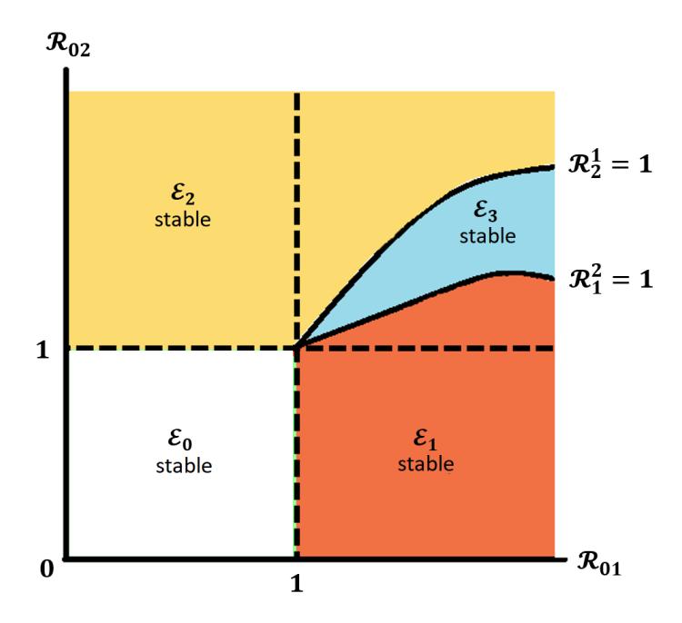
Figure 2: Existence and local stability diagram.
Table 2: Elasticity of R01, R02, R2 1 , and R1 2 .
| E | Ah | Av | µh | µv | α | β1 | β2 | β3 |
|---|---|---|---|---|---|---|---|---|
| R01 | 1 | 1 | −1, 03666 | −0, 64516 | −1, 35484 | 1 | 0 | 0 |
| R02 | 1 | 1 | −1, 03666 | −0, 64516 | −1, 35484 | 0 | 1 | 0 |
| R2 1 | −3, 24263 | −3, 11156 | 2, 26708 | 2, 04974 | 4, 30445 | 0, 38844 | −2, 50000 | −1 |
| R1 2 | 20, 16760 | 20, 02584 | −19, 80177 | −12, 96562 | −27, 22781 | −3, 50000 | 22, 52584 | 1 |
| E | η1 | η2 | q | p | γ1 | γ2 | γ3 | γ4 |
| R01 | 1 | 0 | −0, 00001 | 0 | −0, 96334 | −0, 00001 | 0 | 0 |
| R02 | 0 | 1 | 0 | −0, 00001 | 0 | 0 | −0, 96334 | −0, 00001 |
| R2 1 | 0, 25737 | −3, 50000 | 0, 00001 | 0, 00001 | 0, 71541 | 0, 00001 | 3, 37170 | 0, 00001 |
| R1 2 | −3, 50000 | 23, 66760 | 0, 00001 | −0, 00001 | 2, 40836 | 0, 00001 | −22, 80002 | −0, 00001 |
To enclose our result in this section, we give a sensitivity analysis of R0 respect to the proportion of infected individual who undergoes treatment and fumigation in Figure 3. Based on Table 2, we know that fumigations are the most influential parameter for the system (2). Based on Figure 3(a) we know that the blue area is illustrated in the region where R0 < 1, means malaria superinfection will disappear from populations over time. The region inside the blue area, which separated by the dashed lines (α < α1 and q < q1) are illustrated that both interventions, medical treatment, and fumigation, is should be done to eliminate malaria superinfection from populations. Otherwise, the region outside the blue area which separated by the dashed lines (α > α1 and q > q1) are illustrated that one intervention could be done to eliminate malaria superinfection from populations. The yellow area from Figure 4(a) is illustrated in the region where R0 > 1,
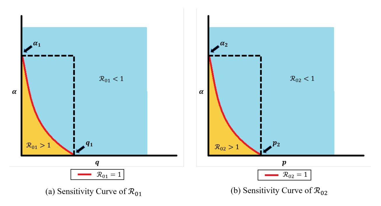
Figure 3: Sensitivity of p, q and α on determining the size of R0, where α1 = 0.19737, q1 = 0.04121, α2 = 0.155574, and p2 = 0.02845.
it means malaria superinfection will always appear in populations over time. Similarly, things to describe Figure 3(b) as before.
Then we can conclude from Table 2 and Figure 3, that fumigation (α) and the proportion of human who get medical treatment (p and q) have a negative relation to R0. While it may seem obvious that high-intensity treatment and fumigation can reduce the value of R0, it is noteworthy that the elasticity of fumigation is significantly higher compared to treatment. This suggests that fumigation is more effective in reducing both the basic and invasive reproduction numbers. Consequently, if we need to choose a single intervention to control the spread of malaria, fumigation would be the optimal choice.
4. SENSITIVITY ANALYSIS ON THE PROPOSED MALARIA MODEL
To simulate the sensitivity of our proposed model (2) respect to the change of parameters, we divide the numerical experiments into four cases, based on the combination of the control reproduction numbers and Figure 2. To conduct the simulation, we use the following parameters value, except it is stated differently depending on the scenario below.
\[A_h = \frac{1000}{72 \times 365}, A_v = \frac{1000}{14}, \mu_h = \frac{1}{72 \times 365}, \mu_v = \frac{1}{14}, \alpha = 0.15, \beta_1 = 0.0015, \beta_2 = 0.001, \beta_3 = 0.09\]\[\eta_1 = 0.7, \eta_2 = 0.75, q = 0, p = 0, \gamma_1 = 0.001, \gamma_2 = 0.3325, \gamma_3 = 0.001, \gamma_4 = 0.3325, N = 1000.\]
Another important step of parameter analysis is using the idea of local sensitivity analysis, we calculate the local sensitivity of each model state concerning model parameters for the model equations 2, the above parameters are used with initial populations S(0) = 800, I1(0) = 120, I2(0) = 80. We compute the model sensitivities using three different techniques: non-normalizations, half normalizations, and full normalizations; see Figures 4–15. This local sensitivity analysis shows how sensitive the state variables respect to a parameter.
Let k as the parameters on model (2), and xi as variables which describe S, I1 or I2 on (2). Then, Nonnormalization is given by
\[\frac{\partial x_i(t)}{\partial k},\]
half-normalization is given by
\[\frac{1}{x_i(t)} \times \frac{\partial x_i(t)}{\partial k},\] and the full-normalization is given by
\[\frac{k}{x_i(t)} \times \frac{\partial x_i(t)}{\partial k}.\]
Interestingly, results provide us further understanding of the model and give one to identify the key critical model parameters.
4.1. Sensitivity analysis when R01 < 1, R02 < 1
To conduct simulation in this section, we use parameter value as in the beginning of this section , except p = 0.7 and q = 0.7 which gave us R01 = 0.00656, R02 = 0.00469. Therefore, we have
\[\mathcal{E}_0 = (S, I_1, I_2) = (1000, 0, 0),\] is locally stable. It can be seen from Figure 4 that from non-normalization sensitivity analysis, susceptible human is very sensitive to the change of β2, while I1 and I2 to µh. Similar results are given from the half normalization in Figure 5. Interestingly, when full normalization sensitivity analysis conducted as shown in Figure 6, we can see that susceptible human is very sensitive to the birth rate of mosquito Av, infection rate on human β2 and infection rate on mosquito η2. On the other hand, infected human no longer sensitive to the infection rate, but now they are sensitive to the proportion of infected human who get hospitalized (p and q), and the recovery rate γ2 and γ4. From this simulation, we can take information that whenever the system will tend to a malaria-free equilibrium, then each variable is very sensitive to the changes in infection rate, especially in the human population.
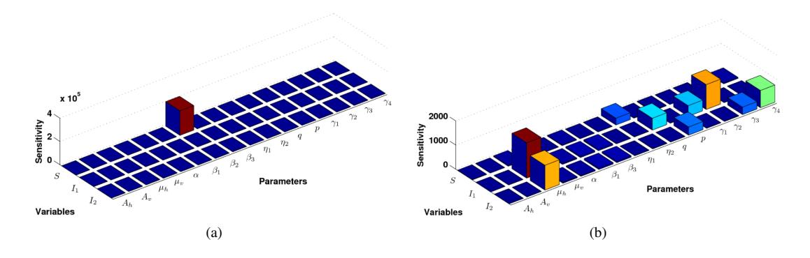
Figure 4: Local sensitivity analysis with non–normalizations in computational simulations when R01 < 1, R02 < 1 (a) the sensitivity of all variables concerning to all parameters, (b) the sensitivity of all variables concerning to all parameters except β2.
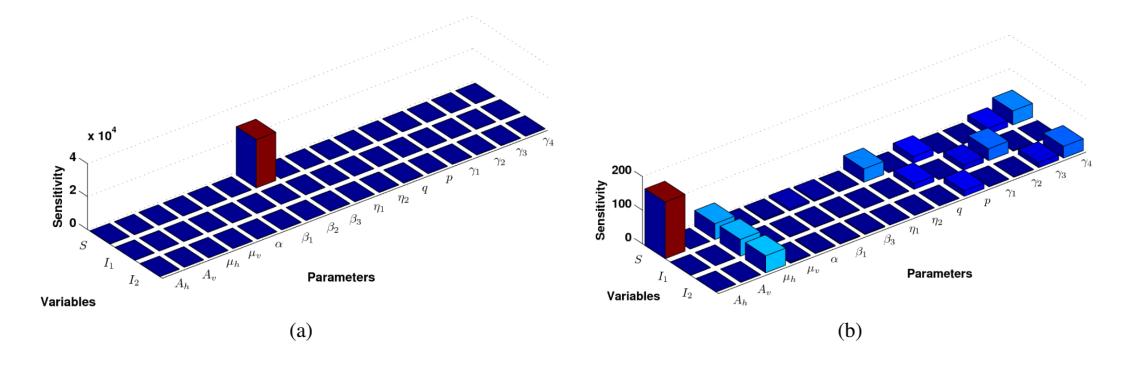
Figure 5: Local sensitivity analysis with half normalizations in computational simulations when \(\mathcal{R}_{01} < 1\), \(\mathcal{R}_{02} < 1\) (a) the sensitivity of all variables concerning to all parameters, (b) the sensitivity of all variables concerning to all parameters except \(\beta_2\).
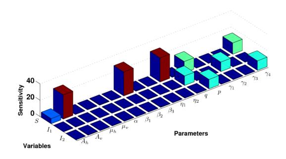
Figure 6: Local sensitivity analysis with full normalizations in computational simulations when \(\mathcal{R}_{01} < 1, \mathcal{R}_{02} < 1\), the sensitivity of all variables concerning to all parameters.
4.2. Sensitivity analysis when \(\mathcal{R}_{01}>1, \mathcal{R}_{02}<1, \mathcal{R}_1^2>1\)
We use mentioned parameters value as mentioned before, except q=0 and p=0.7 which gave us \(\mathcal{R}_{01}=1.47358, \mathcal{R}_{02}=0.00469, \mathcal{R}_1^2=177.32082\). Hence, we have that
\[\mathcal{E}_1 = (S, I_1, I_2) = (702.04850, 10.92198, 0),\] is locally stable. From Figure 7, 8, and 9, it can be seen that infection parameter \(\beta_2\) again is the most influential parameter in the susceptible population. On the other hand, there are three parameters which the most sensitive to determine the size of the susceptible population when full normalization conducted, that are \(A_v, \beta_2\), and \(\eta_2\). From this simulation, we conclude that when the system shows the stability of the endemic equilibrium of plasmodium falciparum only, system (2) is very sensitive to the infection parameter \(\beta_2\) for all type of sensitivity technique.
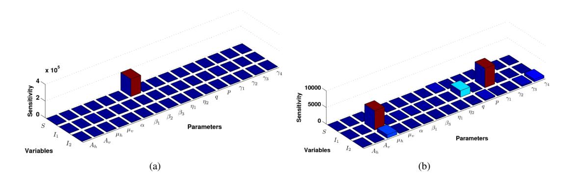
Figure 7: sensitivity analysis with non-normalizations in computational simulations when \(\mathcal{R}_{01} > 1\), \(\mathcal{R}_{02} < 1\), \(\mathcal{R}_1^2 > 1\) (a) the sensitivity of all variables concerning to all parameters, (b) the sensitivity of all variables concerning to all parameters except \(\beta_2\).
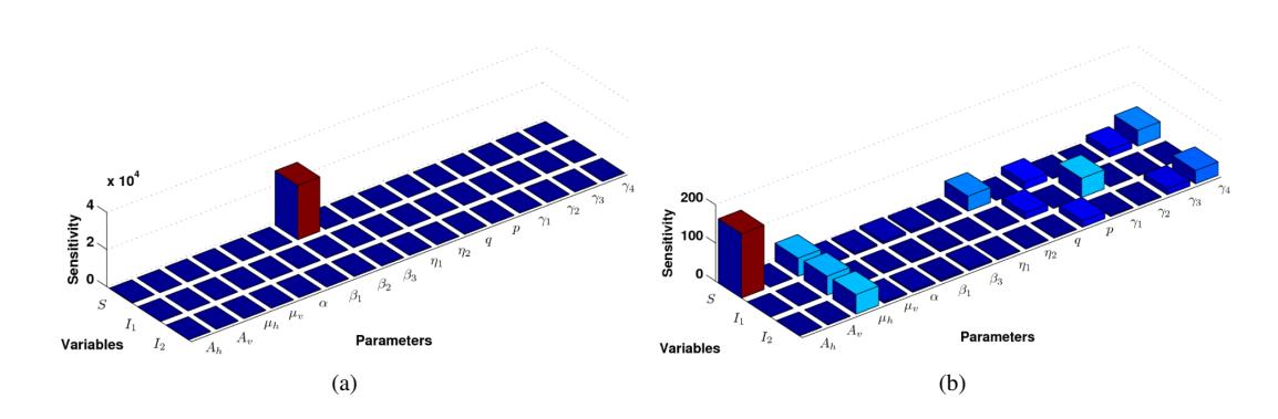
Figure 8: Local sensitivity analysis with half normalizations in computational simulations when \(\mathcal{R}_{01} > 1\), \(\mathcal{R}_{02} < 1\), \(\mathcal{R}_1^2 > 1\) (a) the sensitivity of all variables concerning to all parameters, (b) the sensitivity of all variables concerning to all parameters except \(\beta_2\).
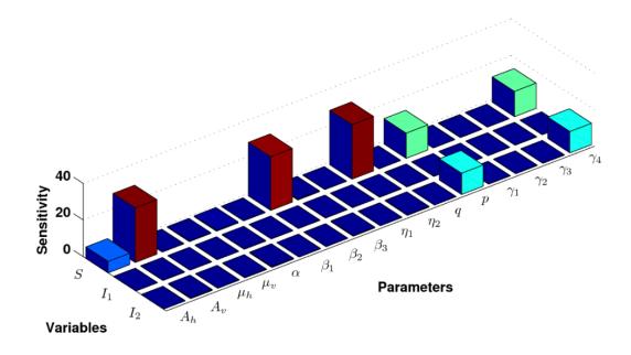
Figure 9: Local sensitivity analysis with full normalizations in computational simulations when \(\mathcal{R}_{01} > 1\), \(\mathcal{R}_{02} < 1\), \(\mathcal{R}_1^2 > 1\), the sensitivity of all variables concerning to all parameters.
4.3. Sensitivity analysis when \(\mathcal{R}_{01} < 1, \mathcal{R}_{02} > 1, \mathcal{R}_2^1 > 1\)
We use mentioned parameters value as mentioned before, except q=0.7 and p=0 which gave us \(\mathcal{R}_{01}=0.00656, \mathcal{R}_{02}=1.05256, \mathcal{R}_2^1=68.04903\). Hence, we have that
\[\mathcal{E}_2 = (S, I_1, I_2) = (955.33340, 0, 1.63734),\] is locally stable. In this section, we provide how our proposed model in (2) sensitive to the change of model parameters, when we set the system stable to the endemic state of plasmodium vivax only. Interestingly, our numerical experiment results in Figures 10, 11 and 12 show similar qualitative results as in section 5.2, that \(\beta_2\) is the most sensitive parameter to the susceptible population for all types of sensitivity analysis.
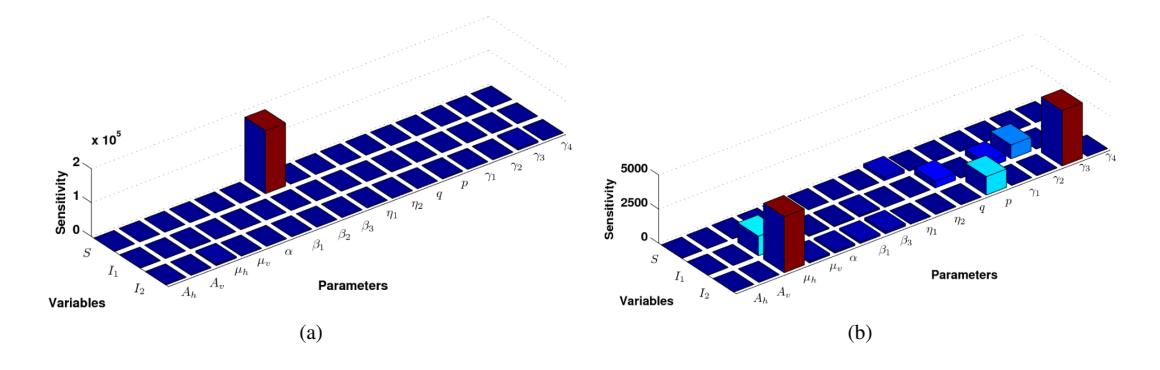
Figure 10: Local sensitivity analysis with non-normalizations in computational simulations when \(\mathcal{R}_{01} < 1\), \(\mathcal{R}_{02} > 1\), \(\mathcal{R}_2^1 > 1\) (a) the sensitivity of all variables concerning to all parameters, (b) the sensitivity of all variables concerning to all parameters except \(\beta_2\).
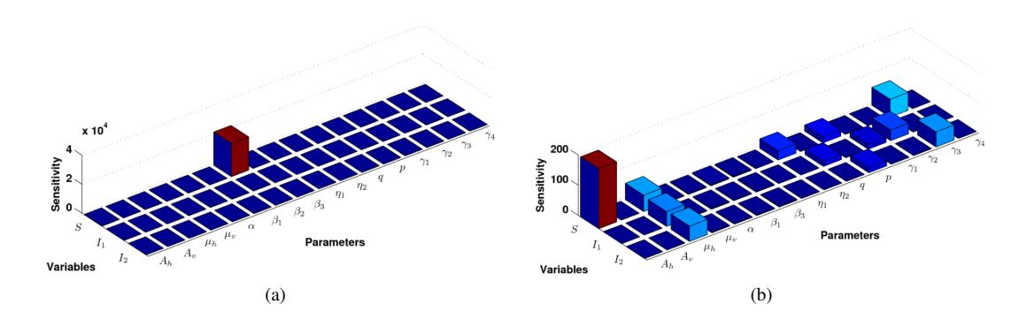
Figure 11: Local sensitivity analysis with half normalizations in computational simulations when \(\mathcal{R}_{01} < 1, \mathcal{R}_{02} > 1, \mathcal{R}_2^1 > 1\) (a) the sensitivity of all variables concerning to all parameters, (b) the sensitivity of all variables concerning to all parameters except \(\beta_2\).
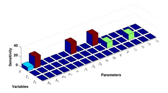
Figure 12: Local sensitivity analysis with full normalizations in computational simulations when \(\mathcal{R}_{01} < 1, \mathcal{R}_{02} > 1, \mathcal{R}_2^1 > 1\), the sensitivity of all variables concerning to all parameters.
4.4. Sensitivity analysis when \(\mathcal{R}_{01}>1,\mathcal{R}_{02}>1,\mathcal{R}_1^2<1,\mathcal{R}_2^1<1\)
We use the mentioned parameters value as mentioned before, which gave us \(\mathcal{R}_{01}=1.47358, \mathcal{R}_{02}=1.05256, \mathcal{R}_1^2=0.22635, \mathcal{R}_2^1=0.49496\). Hence, we have
\[\mathcal{E}_3 = (S, I_1, I_2) = (891.86618, 0.78650, 3.17735),\] is locally stable. When our system set to stable on the coexistence equilibrium, it can be seen that again \(\beta_2\) is very dominant to determine the size of the susceptible population in all types of normalization techniques (Please see Figures 13, 14 and 15). However, we can see that the infected compartments are very sensitive to the proportion of hospitalized individuals, and their recovery rate as shown by non and half normalization techniques.
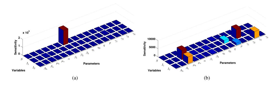
Figure 13: Local sensitivity analysis with non-normalizations in computational simulations when \(\mathcal{R}_{01} > 1\), \(\mathcal{R}_{02} > 1\), \(\mathcal{R}_1^2 < 1\), \(\mathcal{R}_2^1 < 1\) (a) the sensitivity of all variables concerning to all parameters, (b) the sensitivity of all variables concerning to all parameters except \(\beta_2\).
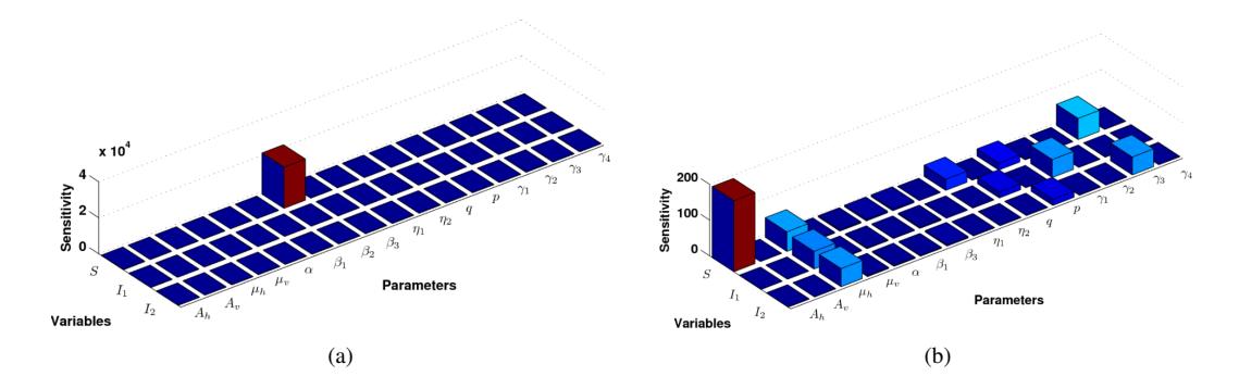
Figure 14: Local sensitivity analysis with half normalizations in computational simulations when \(\mathcal{R}_{01} > 1\), \(\mathcal{R}_{02} > 1\), \(\mathcal{R}_1^2 < 1\), \(\mathcal{R}_2^1 < 1\) (a) the sensitivity of all variables concerning to all parameters, (b) the sensitivity of all variables concerning to all parameters except \(\beta_2\).
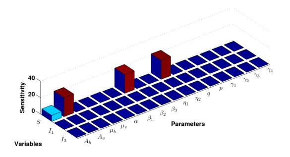
Figure 15: Local sensitivity analysis with full normalizations in computational simulations when \(\mathcal{R}_{01} > 1\), \(\mathcal{R}_{02} > 1\), \(\mathcal{R}_1^2 < 1\), \(\mathcal{R}_2^1 < 1\), the sensitivity of all variables concerning to all parameters.
5. AUTONOMOUS SIMULATION
First autonomous simulation is aimed to see how the proportion of humans infected with Plasmodium falciparum who getting medical treatment affects the dynamics of malaria superinfection transmission in the system (2). The simulation was done with 7 different values of q, from q=0 to q=0.3 with a step size 0.05. Simulation results for variations in the value of q with h=0.05 can be seen in Figure 16. The arrows indicate a direction change from the smallest q value, which is a red graph (q=0.3).
Based on this simulation, it was known that a higher proportion of infected humans with Plasmodium falciparum who getting medical treatment makes the number of infected humans decreases, and malaria superinfection will disappear slowly over the time. Otherwise, the number of susceptible and recovered humans will increase as the proportion of q increases. This indicates that medical treatment can make malaria superinfection disappear from the population over the time.
The next autonomous simulation is aimed to see how the proportion of humans infected with Plasmodium vivax who getting medical treatment affects the dynamics of malaria superinfection transmission in the system (2). The simulation was done with 7 different values of p, from p=0 to p=0.3 with a step size 0.05. Simulation results for variations in the value of p with h=0.05 can be seen in Figure 17. The arrows indicate a direction change similarly as before.
From Figure 17, it is known that a higher proportion of infected humans with Plasmodium vivax who getting treatment makes the number of infected humans with Plasmodium vivax will decrease and malaria superinfection will disappear slowly over time. This also indicates that medical treatment can make malaria superinfection disappear from the population over the time.
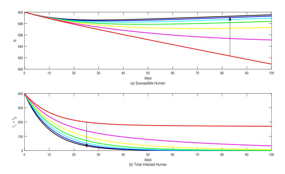
Figure 16: Case Effect of Proportion with Medical Treatment for Plasmodium falciparum (q) with h = 0.05.
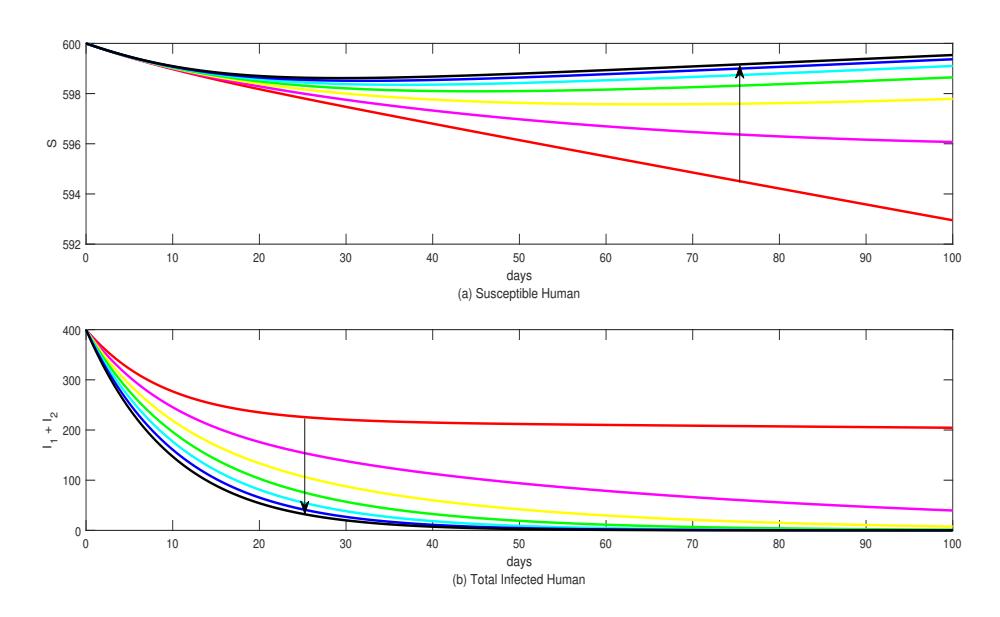
Figure 17: Case Effect of Proportion with Medical Treatment for Plasmodium vivax (p) with h = 0.05.
Furthermore, an autonomous simulation was done to see how fumigation affects the malaria superinfection model in the system (2). The simulation was done with 7 different values of \(\alpha\), from \(\alpha=0\) to \(\alpha=0.3\) with a step size 0.05. To see the urgency of fumigation, we increase number of mosquito becomes ten times larger than human population. Hence, we set \(A_v=10000/(65\times365)\). Simulation results for variations in the value of \(\alpha\) with h=0.05 can be seen in Figure 18.
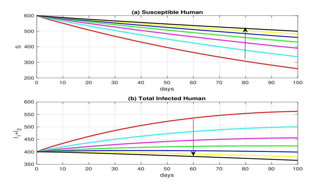
Figure 18: Case Effect of Fumigation (\(\alpha\)) with h=0.05 Respect to Human and Mosquitoes.
It can be seen from Figure 18, a high-intensity of fumigation results in fewer humans being infected due to mosquito bites. Based on this simulation, it was known that a higher intensity of fumigation, can make the total number of infected human is less by mosquito bites and increase the number of susceptible humans. In other words, controlling malaria by fumigation with a high-intensity can make malaria superinfection disappear from the population.
6. CONCLUSION
Mathematical models can provide insight into various aspects of the transmission mechanism of a disease and analyzing the best strategy to prevent the epidemic among the community. Here in this study, we modeled malaria transmission among human and mosquito populations, considering several important factors, such as multiple plasmodium model, superinfection phenomena, fumigation, and treatment as control strategies. Our model describes how superinfection appears from a consecutive bite from mosquito to an individual who already infected before. We construct the model as a seven-dimensional non-linear ordinary differential equation. Since we are interested to see the long time behavior of our system and considering the fast dynamic in a mosquito, we use the Quasi-Steady State Approximation to simplify our model into a threedimensional model. Our findings suggest that controlling the local control reproduction numbers for malaria eradication can not be the only concern for the policymakers since it exists another threshold that describes the interaction between Plasmodium infection. These thresholds called the invasive control reproduction number. Misunderstanding is one of these thresholds that could give into a dominant infection of one Plasmodium. Furthermore, the invasion control reproduction number describes how "tolerance" is an infection between two types of Plasmodium. If one of the invasion control reproduction number is larger than unity, or even both is larger than unity, then coexistence will not occur. Both invasion reproduction numbers should less than unity to guarantee the existence of the coexistence equilibrium point.
Our elasticity analysis on the local and invasive control reproduction numbers indicates that fumigation is the most influential parameter in determining these thresholds. It suggests the potential of fumigation as the intervention to eradicate malaria from the community. However, the effect of fumigation on these thresholds is not the same. Increasing the fumigation rate will reduce the local control reproduction number and invasive control reproduction number of Plasmodium vivax to Plasmodium falciparum, but on the other hand, it will decrease the invasive control reproduction number of Plasmodium falciparum to Plasmodium vivax. Therefore, uncontrolled fumigation could lead to the endemic of malaria with Plasmodium falciparum only, as mentioned in Theorem 3.4. However, although fumigation is the most promising intervention for malaria eradication in our proposed model, combining this intervention with medical treatment for an infected individual will give a better result in malaria eradication, especially in the human population. From analysis on the contour plot of the local control reproduction number, we find that when policymakers want to combine fumigation and medical treatment as the intervention strategy, the order in which the intervention parameters are taken is crucial to determine the level of success of the interventions.
While our model provides insights into the impact of superinfection on malaria transmission, we acknowledge that it does not incorporate incidence data in its calculations. Finding the best-fit parameters for calibration is crucial to enhance our model. Therefore, to further improve our model, we will utilize incidence data to estimate parameter values that align with the observed data trends.
DATA AVAILABILITY
No data were used to support this study.
CONFLICT OF INTEREST
The authors declare no conflicts of interest regarding the publication of this paper.
ACKNOWLEDGMENTS
The authors would like to acknowledge the anonymous editor and reviewers. This research is funded by Directorate of Research and Development, Universitas Indonesia and LPDP with PUTI Q2 matching fund research grant scheme (ID Number: NKB-1402/UN2.RST/HKP.05.00/2022 ).