

1. Introduction
The novel severe acute respiratory syndrome coronavirus (SARS-CoV-2), responsible for the COVID-19 disease, exhibits a highly contagious nature, leading to a substantial number of infections and fatalities worldwide [1], [2]. In comparison to its predecessors, Middle East Respiratory Syndrome (MERS) and Severe Acute Respiratory Syndrome (SARS), this virus demonstrates heightened infectivity, primarily through close contact transmission [3]. Healthcare workers (HCWs) face a particularly high risk of contracting COVID-19 due to their close proximity to infected patients [4]. When an infected individual sneezes, coughs, talks, breathes, or sings, the virus-laden liquid droplets expelled from their mouth or nose can easily disseminate and infect vulnerable individuals [5].
The COVID-19 epidemic was initially identified in Wuhan, China, in December 2019, rapidly spreading and evolving into a global pandemic that has impacted nations across the globe [6], [7]. In Indonesia, the first case of COVID-19 was detected in early March 2020. Subsequently, the Alpha variant (B.1.1.7), initially identified in England in September 2020, triggered the first wave of the COVID-19 epidemic in Indonesia in April 2021. The presence of this variant was initially confirmed on various Indonesian islands, including Sumatra, Java, Bali, and East Kalimantan. Following this, the Beta variant (B.1.351), first detected in South Africa in May 2020, led to the second wave of the COVID-19 epidemic in Bali, Indonesia, also in April
*Corresponding author 2021. In April 2021, the third wave commenced with the first confirmed case of the Delta variant (B.1.617.2) originating from Kepulauan Riau and DKI Jakarta, subsequent to its identification in India in October 2020. Lastly, the Omicron variant (B.1.1.529), first identified in South Africa in November 2021, sparked the fourth wave of the COVID-19 epidemic in December 2021 [8], [9]. The initial detection of the Omicron variant occurred at Wisma Atlet in Jakarta [22].
Prior to the advent of a COVID-19 vaccine, various preventive measures were implemented to curtail the virus's spread, encompassing physical distancing, mask-wearing, and frequent handwashing. Research conducted by [27] has revealed that reducing transmission rates and expediting the identification of infected individuals constitute superior strategies for suppressing the virus's spread. Researchers are confined to analyzing the rate of propagation and exploring potential factors that may exacerbate the number of infections. Following the development of vaccines, studies have been conducted to examine their efficacy. The introduction of vaccines is expected to effectively suppress the virus's rapid transmission. Several researchers have employed the SEIR model to assess the impact of vaccines on curtailing the virus's dissemination. In [29], the integration of quarantine and vaccination within the SEIR model demonstrates that augmenting both quarantine and vaccination rates can significantly reduce disease transmission. Moreover, [28] indicates, without relying on data, that epidemic eradication can only be achieved through a fixed period of immunity. In the absence of vaccines for this pandemic, the model predicts a long-term affliction of a small percentage of the population [30].
The substantial decline in vaccine-induced immunity has prompted considerations regarding the necessity of additional vaccinations. Particularly in Indonesia, the emergence of the Delta and Omicron variants postvaccination has raised concerns regarding vaccine effectiveness and the risk of reinfection. It is imperative for the government to assess the current state of herd immunity before proceeding with additional inoculations, specifically determining whether the threshold of 70% herd immunity has been attained. To shed light on this matter, the present study aims to: (1) develop a transmission model employing vaccinated data as input, (2) ascertain the rate of immunity waning by analyzing vaccination progress, and (3) identify the process (vaccination or recovery) contributing most significantly to achieving optimal immunity levels. We have employed a modified SEIR (Susceptible-Exposed-Infectious-Recovered) model, incorporating a distinct compartment to represent the vaccinated population, referred to as the SEIRV model. This analysis encompasses time-varying parameters and employs cumulative case data to construct an analytical and numerical depiction of the state dynamics.
2. DATASET
As of March 5th, 2021, Jakarta, the capital of Indonesia, has witnessed a total of 346,975 confirmed cases of COVID-19. Among these cases, there are currently 7,173 active cases, while 334,100 individuals have successfully recovered. Regrettably, the city has also reported 5,702 fatalities [11]. These numbers continue to surge, underscoring the urgent need for widespread vaccination efforts to curtail the relentless increase in active cases.
For our research, we utilized data obtained from the official Covid Data in Jakarta source. The data covers the timeframe from March 5th, 2021, to April 2nd, 2022. It spans the period encompassing the initial distribution of vaccines in Indonesia until the completion of our study. It is noteworthy that during this period, the emergence of two new variants, namely Delta and Omicron, was detected. Our study delves into the analysis of daily reported data, as depicted in Figures 1, 2, and 3. These figures unveil two significant spikes in case numbers, one occurring in June 2021 and the other in January 2022. These sudden surges in COVID-19 cases coincided with the identification of the Omicron and Delta variants. The aforementioned surge gave rise to a notable escalation in both the number of fatalities and recoveries. This phenomenon is rational, as it augments the probability of either succumbing to the illness or achieving a state of recuperation.
Following the detection of these variants, the highest number of daily positive cases was recorded. For the Delta variant, the peak was reached on July 12, 2021, with a staggering 14,619 cases reported. As for the Omicron variant, its highest daily case count of 15,825 occurred on February 6th, 2022. However, it should be noted that not all of these cases can be definitively attributed to the Omicron variant.
The outcomes of the research unveil a notable disparity in antibody titers between severe breakthrough infections and mild breakthrough infections. Specifically, the antibody titers induced by Delta breakthrough infections were found to be 10.83 times higher than those of Omicron breakthrough infections. This suggests that Delta infections elicit a significantly stronger immune response, thereby offering greater protection against
reinfection or infection from future variants [10]. Nevertheless, in our study, we have focused on utilizing the data without distinguishing individuals infected with either the Delta or Omicron variants.
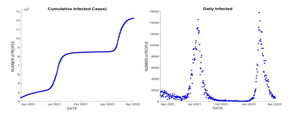
Figure 1: Daily and cumulative data plot of infected cases.
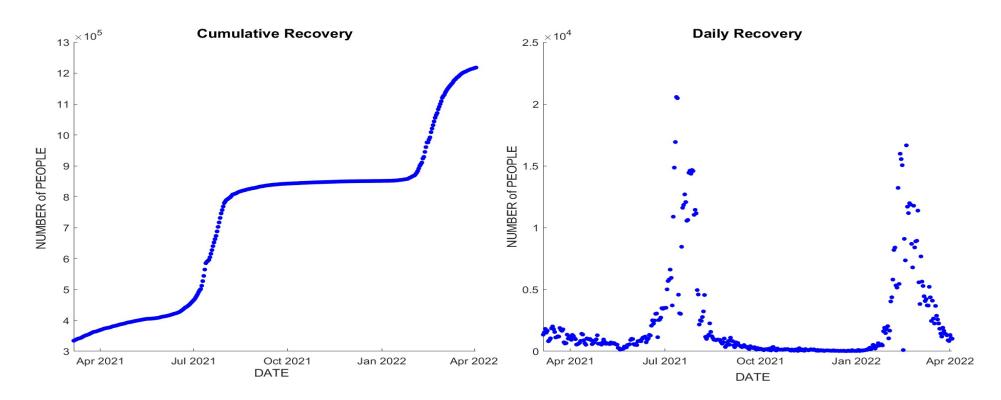
Figure 2: Daily and cumulative data plot of recovery cases.
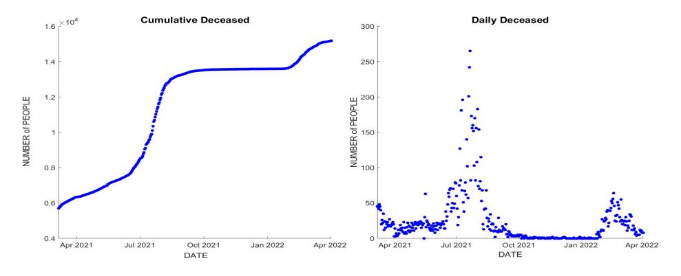
Figure 3: Daily and cumulative data plot representing the deceased individuals.
Upon careful examination of the three aforementioned plots, one can discern that the cumulative data graphs pertaining to active cases, recoveries, and deaths exhibit a seamless trajectory, characterized by a gentle S-shaped curvature. This significant observation forms the foundation for the utilization of Richard's curve in the present study. Further elaboration on this matter will be expounded upon in the subsequent section.
3. MATHEMATICAL MODEL
We commence with the SEIR transmission model of COVID-19, encompassing the susceptible compartment denoted as S, the exposed compartment represented by E, wherein individuals undergo an incubation period, the infected and infectious compartment denoted as I, the recovered compartment denoted as R, and an additional compartment for individuals who have been vaccinated, denoted as V . The depiction of these compartments in the SEIRV model can be observed in Figure 4. In order to construct this diagram, certain assumptions are required, which shall be elucidated as follows.
Assumptions
One of the challenges encountered in constructing models lies in the task of translating real-world phenomena into mathematical representations that can faithfully encapsulate their inherent complexity. Thus, in order to render the model manageable and practicable, it often becomes imperative to introduce simplifying assumptions. However, it is crucial that these assumptions do not compromise the integrity and pertinence of the research. Within the scope of this study, we have taken into account the following assumptions:
- 1) Vaccination is exclusively administered to individuals belonging to compartments S and E.
- 2) The recruitment rate remains constant.
- 3) Age is assumed to be uniformly distributed.
- 4) The human lifespan is considered to be 70 years.
- 5) Individuals who have recovered may only receive vaccination three months subsequent to their official recovery declaration.
- 6) Only data officially recorded by the government is taken into consideration.
- 7) There are no occurrences of infection following the primary vaccine (first and second dose).
- 8) Every vaccine is assumed to provide equal efficacy.
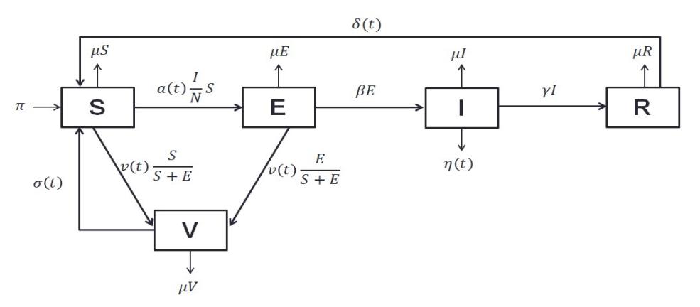
Figure 4: Compartment diagram of SEIRV model.
The parameters β, γ, and µ represent constant values, while a(t), v(t), σ(t), η(t), and δ(t) denote timedependent parameters. A comprehensive explanation of these parameters can be found in Table 1. Each arrow depicted in Figure 4 signifies the dynamic changes occurring over time between the compartments. It should be noted that individuals previously in compartment R can regain susceptibility and become re-infected by the virus due to the gradual waning of natural immunity following recovery.
In accordance with our assumptions, individuals eligible for vaccination originate from compartments S and E, representing the uninfected population. Subsequently, those who receive the vaccine acquire temporary
immunity against the virus. However, once this immunity diminishes, vaccinated individuals once again become susceptible. The governing equations of SEIRV model can be formulated as follows.
\[\frac{dS}{dt} = \pi + \delta(t) + \sigma(t) - v(t) \left(\frac{S}{S+E}\right) - a(t) \frac{I}{N} S - \mu S,\tag{1}\]
\[\frac{dE}{dt} = a(t)\frac{I}{N}S - v(t)\left(\frac{E}{S+E}\right) - \beta E - \mu E,\tag{2}\]
\[\frac{dI}{dt} = \beta E - \gamma I - \eta(t) - \mu I,\tag{3}\]
\[\frac{dR}{dt} = \gamma I - \delta(t) - \mu R,\tag{4}\]
\[\frac{dI}{dt} = \beta E - \gamma I - \eta(t) - \mu I, \tag{3}\] \[\frac{dR}{dt} = \gamma I - \delta(t) - \mu R, \tag{4}\] \[\frac{dV}{dt} = v(t) - \sigma(t) - \mu V. \tag{5}\]
Table 1: Description of SEIRV Model Parameters.
| Parameter | Description | Value | Reference |
|---|---|---|---|
| β | Incubation Period | \(\frac{1}{6}\) | [15] |
| \(\gamma\) | Infection Period | \(\frac{\Upsilon}{14}\) | [21] |
| \(\mu\) | Natural Death Rate | \(\frac{1}{70 \times 356}\) | adjusted |
| v(t) | Daily Number of Vaccinated People | data | [11] |
| \(\eta(t)\) | Daily deceased individuals by infections | data | [11] |
| \(\sigma(t)\) | Daily Vaccine-induced-immune-compromised individuals | - | estimated |
| \(\delta(t)\) | Daily Number of People Loosing their Natural Immunity | - | estimated |
| a(t) | Infection Rate | - | estimated |
The initial two parameters elucidate the incubation and infection periods of COVID-19, respectively, with regard to the transmission of the disease. The incubation period signifies the span in which an afflicted individual remains devoid of symptoms and non-transmissible until the commencement of disease manifestations, whereas the infection period indicates the timeframe during which an infectious person can transmit the disease. As a general rule, the infection period tends to surpass the incubation period in duration. The natural mortality rate parameter, conversely, quantifies the anticipated number of fatalities arising from inherent causes during the COVID-19 epidemic. This parameter is denoted as "adjusted," as it will be tailored to the specific research location. Its significance lies in the evaluation of the overall impact of the pandemic on the population and healthcare system.
Moreover, v(t) captures the daily count of individuals vaccinated within the population. The eligible individuals for vaccination are those who are not currently infectious. However, in reality, this group may consist of individuals from the susceptible population or those who have been exposed to the virus but have not yet developed symptoms. Differentiating these two populations from infected individuals is challenging and unpredictable, as infected individuals may exhibit immediate symptoms. Therefore, we employ a ratio of the vaccination parameters, whereby a proportion of vaccinated individuals originates from the susceptible population, while the remainder comes from the exposed population.
The values of v(t) and \(\eta(t)\) can be readily derived from the data, particularly from the cumulative data. However, for \(\delta(t)\) and \(\sigma(t)\), a specific transformation is employed, which will be elucidated in the subsequent section. It should be noted that the unobservable parameter a(t) remains unknown. This parameter is designated as a time-dependent entity to accommodate the intervention procedure and will be evaluated using the generating operator.
4. ESTIMATING PARAMETERS
In Section 3, we have expounded upon the model and elucidated the parameters that have been duly considered for the purposes of this study. Within this section, we shall now endeavor to ascertain the numerical values of said parameters. To get the value of each parameter, we fit the cumulative each case data by using the Generalized Linear Growth Model (GLGM):
\[f(t; \theta_1, \theta_2, \theta_3, \xi) = \frac{\theta_1}{(1 + \xi e^{-\theta_2(t - \theta_3)})^{\frac{1}{\xi}}},\] which is widely known as Richard's Curve [15], [24]. In this study, we use empirical fitting 3-layer generalized Richards Curve to estimate the data.
• Daily Number of Fully-Vaccinated Individuals (v(t))
The figure on the left-hand side of Figure 5 depicts the cumulative data, which has been skillfully fitted using the 3-layer generalized Richard curve. Additionally, we have thoughtfully provided a 90% confidence interval to further enhance the reliability of the representation. On the right-hand side, we present the daily vaccinated data, denoted as v(t), obtained through differentiation of the cumulative function with respect to time. The corresponding figure on the right also includes a 90% confidence interval, lending additional credibility to the results. Furthermore, the meticulous calculations yield a noteworthy Sum of Squared Error (SEE) value of 3.0928. From Figure 5, we observe that the number of fully vaccinated individuals has experienced two spikes. The Indonesian government promotes the importance of vaccination from May 2021 until August 2021, and increased public awareness about the severity of COVID-19 disease to reduce positive cases.
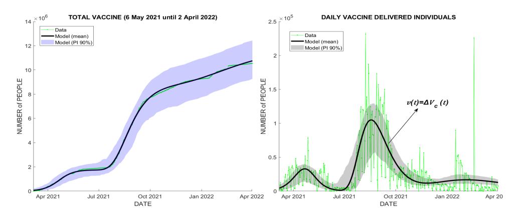
Figure 5: Daily number of fully vaccinated individuals.
• Daily Number of Deceased (η(t))
In a similar fashion to the approach used for determining v(t), we employ differentiation with respect to time to derive the daily number of deceased, denoted as η(t), as illustrated in Figure 6. Upon performing the SSE calculation, a value of SEE 1.1497 is obtained. The figure unmistakably reveals the presence of two prominent peaks. The first peak is observed in August 2021, coinciding with the commencement of the spread of the Delta variant. The second peak emerges in February 2022, corresponding to the transmission of the Omicron variant within Indonesia.
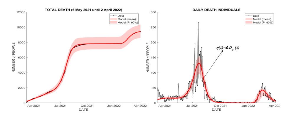
Figure 6: Daily number of deceased.
• Daily Number of People Loosing their Natural Immunity (δ(t, Tn))
Since the value of the δ(t), parameter is time-dependent, we cannot independently state that this value will change at every time t. To obtain the value of δ(t), we perform the following steps:
- 1. Consider the simulation for T days starting at day t = 0. We derive the formula that estimates δ(t).
- 2. Consider the increment of Total Recovery (RC ) from day t = 0 to t = 1.
- 3. Let ∆R0 represent the number of people that occupies the natural immunity from t = 0 to t = 1.
- 4. Assume that the natural immunity loses (on average) for only Tn days, meaning that ∆R0 individuals that are recovered at t = 0 will become re-vulnerable after Tn days.
- 5. Hence, δ(t = Tn) = ∆RC0
- 6. Taking it continuously, we have
\[\delta(t + T_n) = R_C'(t),\] or
\[\delta(t) = R_C'(t - T_n).\]
Eventually, we can get the estimated δ(t) as in Figure 7 by getting the formula of RC fitting the data to Richard's Curve, with SSE is 2.7189. In more refined language, we can determine the function δ(t) by initially performing a differentiation of the cumulative data function, denoted as RC , with respect to time. Subsequently, this differentiated function is right-shifted to the extent of Tn, where the value of Tn utilized is precisely 90 days [13]. This implies that the protective effects of natural immunity fade away within a span of 90 days subsequent to recuperation from the infection. From the right side of Figure 7, it can be seen that there are two spikes. The highest spike occurs around August 2021 when the Delta variant begins to spread, while in February 2022, the Omicron variant begins to spread, leading to another spike.
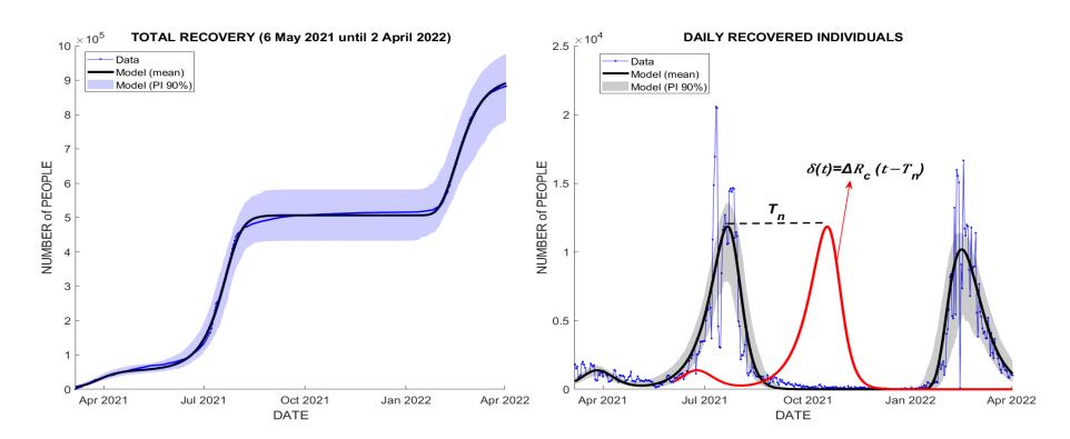
Figure 7: Daily number of people loosing their natural immunity (δ(t, Tn)) with Tn = 90 days [13].
• Daily Number of People Loosing their Vaccine-Induced Immunity (σ(t, Tv))
Similar to finding the δ(t) value, the σ(t) value is determined by shifting the vaccinated data by Tv. This is because over time Tv, people who are vaccinated will start to lose their immunity due to the waning of the vaccine as illustrated in Figure 8, with the SEE is 3.0928. In this context, Tv is predetermined as 180 days according to Feikin [12]. Consequently, the efficacy of the vaccine-induced immunity diminishes after the expiration of 180 days post-vaccination. Nevertheless, it is noteworthy that our findings do not exhibit dual peaks akin to those observed in δ(t), owing to the inherent constraints imposed by the data available for this study.
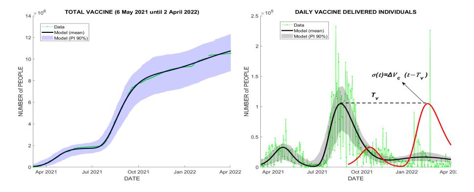
Figure 8: Daily number of people losing their vaccine-induced immunity (simulation) with Tv = 180 days [12].
5. NUMERICAL RESULT
Given the availability of daily data on vaccinated individuals from March 2021 onwards, and considering our previous discussion where we adjusted the data temporally to obtain certain parameter values, we commenced conducting simulations spanning from October 2021 to April 2022. Before conducting the simulation, we will first describe each compartment and the formulation used.
• Cumulative Case (K)
The prevalent global challenge lies in the accurate recording and timely reporting of daily COVID-19 cases, leading to a dearth of dependable data. The complexity of predicting the virus's spread is compounded by the fluctuation in daily cases, as erroneous data fitting can distort the outcomes. To tackle this issue, numerous countries are relying on cumulative data to derive strategic indicators, leveraging its smooth profile for more precise fitting. Although the detailed transmission patterns are obscured in cumulative data, they can be retrieved by identifying the appropriate generating operator. Among the most effective methods for fitting the S-curve shape of cumulative data is Richard's curve, which furnishes a valuable tool for predicting the propagation of COVID-19 and guiding public health policies. The construction of the generating operator commences with the definition of the supplementary compartment K(t), representing the cumulative cases at time t. Cumulative cases are defined as the total count of individuals who have contracted the infection up to a given time point, denoted as time t. This count is derived by aggregating the daily figures of new infections \((I_C)\), deaths \((D_C)\), and recoveries \((R_C)\). It is worth noting that these figures are extracted from the authentic data sources referenced in section 2. Mathematically, this can be expressed as:
\[K = D_C + R_C + I_C, (6)\]
where
\(D_C\): Total daily deceased individuals due to COVID-19 (based on data)
\(R_C\): Total daily recovery (based on data) \(I_C\): Total active cases (based on data)
To obtain daily data, we will compute the cumulative case differentiation with respect to time. Since we are utilizing actual cumulative data, the retrieval of daily figures can be described as follows: firstly, it is evident that the daily number of deaths can be directly obtained by calculating the derivative of the cumulative death data, denoted as \(D_C\), and by assuming \(\mu I\) as the semblance of \(D_C\). Secondly, the daily number of recoveries depends on the rate of the infected population (as recovery is declared after becoming free from infection). Lastly, the daily number of active cases is obtained from the exposed population (as infection follows exposure to the virus) and then subtracted from the daily numbers of recoveries and deaths. Mathematically, this can be represented as follows:
\[\begin{split} \frac{dD_C}{dt} &= \eta(t), \\ \frac{dR_C}{dt} &= \gamma I, \\ \frac{dI_C}{dt} &= \beta E - \gamma I - \eta(t). \end{split}\]
Hence.
\[\frac{dK}{dt} = \frac{dD_C}{dt} + \frac{dR_C}{dt} + \frac{dI_C}{dt} = \beta E. \tag{7}\]
Building upon this equation, it can be inferred that the quantity of daily cases is contingent upon the extent of virus exposure. This rationale holds true as infected and deceased individuals are invariably preceded by exposure to the virus.
Exposed (E)
From Equation (7) we can straightforward get the explicit formula for E as follows:
\[E(K) = \frac{1}{\beta} \frac{dK}{dt}.\] (8)
• Vaccinated (V)
Recall the equations of the system. Last equation gives us:
\[\frac{dV}{dt} = v(t) - \sigma(t) - \mu V,\tag{9}\] which can be solved independently by knowing the values of v(t), \(\sigma(t)\) and \(\mu V\).
• Infected (I) and Recovery (R)
After obtaining the dynamic of E, we consider equations (3) and (4) in the system:
\[\frac{dI}{dt} = \beta E - \gamma I - \eta(t) - \mu I,\]
\[\frac{dR}{dt} = \gamma I - \delta(t) - \mu R.\]
Since we have the values of these constants and the heterogeneous term, then I and R can be evaluated simultaneously.
• Susceptible (S)
The susceptible individuals over time can be calculated by using the following equation:
\[N = S + E + I + R + V.\]
We then evaluate N by considering the following equation:
\[\frac{dN}{dt} = \pi - \mu N.\]
It can be seen that the population is not constant because it is affected by the natural death rate and recruitment rate.
5.1. Cumulative Case Fitting
We employ the three-layer generalized Richards curve to effectively model the data. The disparities between the fitted curve and the empirical observations are negligible, thereby affirming a commendable fit. In this regard, equation (6) is specifically utilized in the cumulative case fitting process, yielding outcomes visually depicted in Figure 9, where the SSE value is 2.2838.
5.2. Daily Cases Fitting
Let \(K(t_i)\) be denoted by \(K_i\). We estimate the daily cases with the forward-time scheme:
\[\frac{dK_i}{dt} = \frac{K_{i+1} - K_i}{\Delta t}.\]
The curve fitting results in Figure 9 show that the curve is well-fitted to the data.
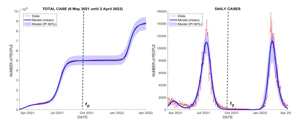
Figure 9: Cumulative and daily cases curve fitting.
5.3. E, I, R, and V Simulation
Based on the simulation results depicted in Figure 10, notable trends can be observed regarding the compartments E, I, R, and V . It is evident that the exposed compartment, E, experienced a surge in February 2022, followed by a subsequent increase in the number of infected individuals, I. In parallel, the count of individuals who has recovered, represented by the compartment R, exhibited a rise towards the end of January, with expectations of a decline within the next 90 days, approximately by May 2022.
As evidenced by Figure 10, the number of fully vaccinated individuals displayed a progressive growth from October 2021 to January 2022. The immunity conferred by the vaccine offers protection for a period of 180 days, commencing from the day of initial vaccination. The Indonesian government stipulates that herd immunity can be achieved if a minimum of 70% of the total population possesses immunity either from infection or through vaccination. By combining the R and V compartments, it is evident that herd immunity was attained during the period spanning October 2021 to January 2022. However, as depicted in Figure 10, the immunity level has started to decline since February 2022 due to the waning effect of the vaccine. Consequently, it is advisable to initiate the administration of booster doses for the COVID-19 vaccine.
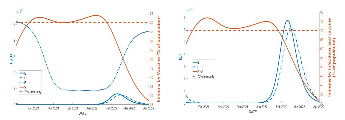
Figure 10: Simulation results for E, I, R, and V.
5.4. S and N Simulation
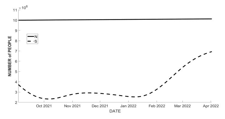
Figure 11: Simulation results for S and N.
Although Figure 11 displays a marginal significance, it reveals the dynamic nature of the N and S compartments. As previously indicated, the N compartment experiences fluctuations due to recruitment rates and natural deaths, while the S compartment represents a susceptible population susceptible to the virus.
Notably, Figure 11 illustrates a substantial surge in the S compartment subsequent to February 2022. This change aligns with the observed waning of immunity during the corresponding timeframe, as illustrated in Figure 10. It is noteworthy to mention that this study does not account for a vaccine booster, consequently resulting in a subsequent increase in the number of susceptible individuals once the vaccine's efficacy wanes. Consequently, these individuals become vulnerable to COVID-19 infection once again.
5.5. Infected Rate (a(t)) Simulation
Based on equation (2), we can obtain the following equation:
\[a(t) = \frac{\left(\frac{dE}{dt} + v(t)\left(\frac{E}{S+E}\right) + \beta E + \mu E\right)N}{SI}.\]
Having acquired the values for all variables, we proceed to conduct a simulation of a(t) with the aim of illustrating the infected rate, as depicted in Figure 12. The outcomes reveal a notable peak in transmission rate transpiring during the months of January and February 2022. Interestingly, this aligns precisely with the timeframe characterized by the waning of the vaccine (Figure 10). Subsequently, a decline in the transmission rate becomes apparent, potentially attributable to the influence of the vaccine booster administered by the government towards the conclusion of January 2022.
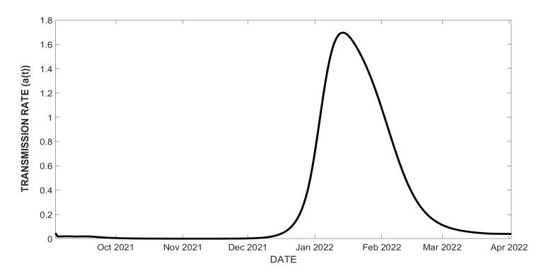
Figure 12: The trajectory of the infection rate, denoted as a(t).
5.6. Effect of a(t) on E and I
In this section, we illustrate the impact of the transmission rate a(t) on the compartments E and I. As depicted in Figure 13, elevating the transmission rate results in a subsequent rise in the population of exposed individuals, followed by an increase in the number of infected and infectious individuals. This phenomenon is plausible since the transmission rate signifies the extent of virus transmission, implying that augmenting the transmission rate would engender a surge in individuals being exposed (E), subsequently leading to a rise in individuals contracting the infection (I).
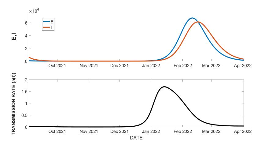
Figure 13: The influence of a(t) on E(t) and I(t).
6. EFFECTIVE REPRODUCTIVE RATIO
In the scenario of a constant infection rate, denoted as a(t) = α, the fundamental reproductive ratio, commonly referred to as R0, encapsulates the average quantity of subsequent infections anticipated to arise from a solitary infected individual at the onset of an epidemic [25]. The pre-vaccination value of R0 is expressed as:
\[R_0 = \sqrt{\frac{\alpha\beta}{(\beta + \mu)(\gamma + \mu)}}.\]
This value assumes paramount significance as it serves to ascertain the trajectory of an outbreak, whether it will escalate or subside with the passage of time. To elucidate, if the value of R0 exceeds 1, it signifies that each infected individual is expected to transmit the disease to more than one person on average, thereby indicating an ongoing expansion of the outbreak. Conversely, if R0 falls below 1, it implies that the disease is likely to dwindle gradually, since each infected individual will, on average, transmit the disease to fewer than one person.
Nonetheless, when we introduce a time-dependent transmission rate, as observed during the COVID-19 pandemic, relying solely on the basic reproduction ratio is no longer sufficient to accurately monitor the progression of transmission. In order to address this challenge, we can employ the effective reproduction ratio (Rt), which takes into consideration the time-varying transmission rate as well as the proportion of susceptible individuals within the population. The formula for Rt encompasses the transmission rate at a specific time t, denoted by a(t), in conjunction with other parameters such as the incubation period (β), the infection period (γ), the natural death rate (µ), and the fraction of susceptible individuals in the population at time t, denoted by S(t)/N(t). The corresponding effective reproduction ratio can be expressed as follows.
\[R_t = \sqrt{\frac{a(t)\beta}{(\beta + \mu)(\gamma + \mu)}} \times \frac{S(t)}{N(t)}.\]
The determination of Rt is achievable through the utilization of the next-generation matrix technique, thereby obviating the need for the presupposition of a disease-free populace [26]. This method proves to be considerably more precise when it comes to monitoring the evolution of transmission during an ongoing epidemic. Depicted in Figure (14) is the temporal representation of the effective reproduction ratio. As the count of susceptible individuals within the population diminishes, the value of Rt likewise declines, signifying a deceleration in the transmission rate. Conversely, an escalation in the magnitude of Rt would suggest a resurgence of the epidemic.
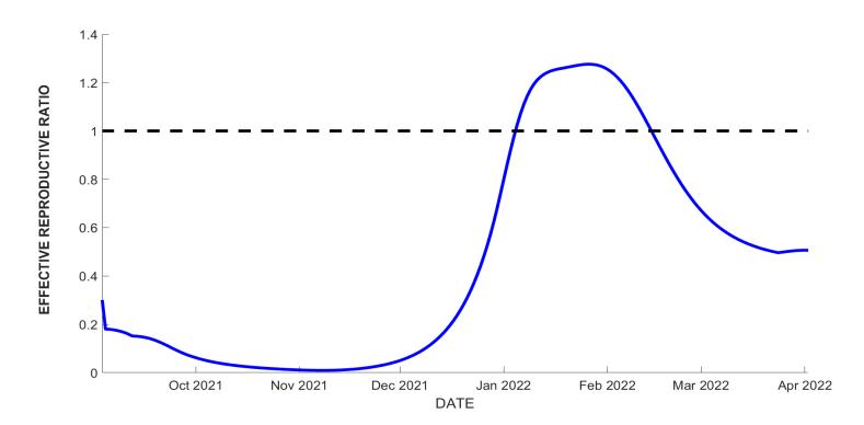
Figure 14: Effective reproductive ratio, denoted as Rt.
7. DISCUSSIONS AND CONCLUSIONS
In this study, we have undertaken an analysis of the impact of primary vaccines on the dynamics of active COVID-19 cases. Additionally, we have compared the strength of immunity derived from vaccines to natural immunity, and have made predictions regarding the optimal timing for administering additional vaccines. The simulation was conducted using data from October 2021 to April 2022, as we aimed to encompass the effective period of the vaccine, starting from the first day of distribution, in order to obtain the necessary parameters. It is important to note, however, that our model does not differentiate the data based on the specific type of vaccine used. In reality, different vaccines may possess varying characteristics and levels of effectiveness. Therefore, by not segregating the data according to vaccine type, our study may not provide a comprehensive understanding of the individual contributions of each vaccine to herd immunity.
To address these considerations, we propose an innovative enhancement to the SEIR model, introducing a new compartment called the vaccine compartment (V ). This novel model incorporates three fundamental elements: cumulative data, the Richard curve, and the proposed compartmental model. The primary objective of the dynamics generator is to fit the empirical cumulative data to the Richard Curve (K), subsequently establishing the relationship between K and the other state dynamics within the SEIRV model. However, it is worth noting that our model assumes that individuals do not contract COVID-19 after receiving the primary vaccine. In reality, however, there exists a possibility, albeit low, of individuals being infected even after vaccination.
In order to generate all the state dynamics, we consider the empirical data of cumulative cases. This choice is motivated by the consistently increasing nature of this data, which facilitates the selection of an appropriate cumulative function. Our implementation employs a three-layer Richard Curve, as the cumulative curve exhibits a three-layer S-curve pattern. By integrating this dynamics generator into the updated SEIRV model, we are able to generate all state dynamics and estimate the effects of primary vaccines on the dynamics of active COVID-19 cases. A significant advantage of adopting the dynamics generator approach is that it allows for the evaluation of time-dependent transmission rates. As evident from our simulation results, the transmission rate significantly influences the number of cases. An increase in the transmission rate leads to a corresponding rise in the exposed and infected population. Conversely, a decrease in the transmission rate is followed by a reduction in the number of exposed and infected individuals, indicating a mitigation of COVID-19 spread. These findings are consistent with the conclusions reached by Ndii et al. [27].
The simulation results obtained from the SEIRV model reveal that natural immunity plays a more dominant role compared to vaccine-induced immunity. Despite the implementation of a vaccination program, achieving the target of herd immunity (70%) takes place between October 2021 and February 2022. However, it is important to note that vaccine effectiveness wanes in February 2022, necessitating the administration of a booster dose.
This innovative compartmental model offers a more comprehensive comprehension of the transmission dynamics of COVID-19, thus aiding in the formulation of appropriate policies and strategies to control and prevent the virus's spread. By considering the influence of primary vaccination on the epidemic's dynamics, the dynamics generator approach provides valuable insights into the potential effects of vaccination programs in curbing the transmission of COVID-19. Consequently, this discovery suggests that future research and public health policies should prioritize the investigation and implementation of booster vaccine strategies to enhance and sustain the effectiveness of COVID-19 vaccination programs.
ACKNOWLEDGMENTS
The authors wish to express their gratitude to LPDP-Ministry of Finance of the Republic of Indonesia for the scholarship of the Magister Program at Bandung Institute of Technology, as well as Research and Technology Transfer Office, Bina Nusantara University as a part of Bina Nusantara University's International Research Grant 2023 through the corresponding author [grant no. 029/VRRTT/III/2023] for the financial support in conducting this research.