

1. INTRODUCTION
Orangutans are a type of great ape that only live on the continent of Asia, namely in Indonesia and Malaysia [17]. Orangutans are also endangered animals in Indonesia that are protected by law in order to keep their population alive. The existence of orangutans is closely related to vulnerable living communities and unique ecosystem processes [9]. The extinction of orangutans is caused by various things, one of which is the destruction of forests as orangutan habitat. Destruction of forests is carried out by humans for multiple reasons, one of which is agricultural expansion [12]. Another factor that causes the extinction of orangutans is human behavior in hunting wild animal meat which should be prohibited by government policy [5]. The orangutan's role in the ecosystem includes the welfare of the community around the forest so the orangutan is called an umbrella species, namely a species whose sustainability affects the sustainability of the ecosystem where the species is found [7],[3]. Therefore, policies are needed to maintain the existence of forests as habitats for endangered wildlife [6].
One of the species is Pongo abelii, which is an orangutan native to Sumatra. Based on references [14], it was estimated that there were around 14,000 Pongo abelii populations in 2016. The male Pongo abelii can grow to a mass of 90 kg, while the female is relatively smaller with a mass of 50 kg [8], [16]. Pongo abelii has a thinner body, a longer face, and longer and paler hair than the Borneo orangutan. The diet of Pongo abelii are fruit and insects [10].
The longest reported orangutan average interbirth interval (IBI) was 9.3 years [18]. Too long an IBI duration may hamper the growth of the orangutan population. There are numerous threats to the survival of orangutans, including the removal or loss of orangutans from the population and habitat loss [14]. Habitat loss (destruction of forests) causes a reduction in carrying capacity so that orangutans are threatened with no place to live. Part of this is happening due to illegal logging and fires/burning forests. Furthermore, considering that human behavior towards forest destruction is increasing, action is needed to inhibit this action. The protection of orangutan habitat must be regarded as a conservation strategy [13]. Therefore, in this study, we will focus on simulating the addition of carrying capacity. There are very few studies on population dynamics with
*Corresponding author
carrying capacity that changes with time. In fact, there are changes in orangutan habitat areas over time due to various factors [8]. So, we will examine the positive impact of increasing the carrying capacity on the preservation of the Pongo abelii population through the formulation of a mathematical model consisting of two compartments, namely the orangutan population and carrying capacity.
2. MODEL FORMULATION
The following model that we will use is obtained by adopting the Verhulst logistic model [15], [2]:
\[\frac{dN}{dt} = (r - \frac{q}{N_0})N(1 - \frac{N}{K}),\tag{1}\]
\[\frac{dK}{dt} = -sK + b. (2)\]
Definition and units:
N: orangutan population [orangutans]
\(N_0\): initial orangutan population [orangutans]
K: carrying capacity [orangutans]
r: growth rate [1/year]
q: loss of orangutans from the population for one year [orangutans]
s: loss of carrying capacity [1/year]
b: rate of addition of carrying capacity (e.g. reforestation) [orangutans/year]
We model two aspects: the number of orangutan population and carrying capacity. There are five parameters that we consider, namely r, q, s, b, and \(N_0\). We got all of these parameter values from [14] published in 2016. The parameter r is the initial growth rate that we obtained from [14], with the value of r being assumed to be the same for Sumatran orangutans (r=0.014). However, various problems threaten the orangutan population, and from [14], we get data in the form of the number of orangutans decreasing every year in each area caused by poaching as trade, conflict killing, hunting/food, wounding, and fire. We sum them up and name it as q. In this study, we assume that the actual growth rate of orangutans is \(r-\frac{q}{N_0}\), where \(N_0\) is the initial condition of the number of orangutan populations in each area recorded from [14]. s is a parameter of the rate of forest degradation that occurs with different values in each area. s is an additional simulation parameter that we run to predict the growth rate of carrying capacity in certain areas whose value is constant and does not depend on the area.
In terms of the growth rate of orangutans, we use the Verhulst logistic model [15], [2] with K as the carrying capacity for orangutans. Since the growth rate r does not include other factors, we modify it by reducing the \(\frac{qN}{N_0}\) factor in rN. The value for q and \(N_0\) can be seen in Table 1. Inspired by [11], [1], we assume that the carrying capacity is always changing. In this case, we use the -sK factor because the rate of reduction in carrying capacity is considered proportional to the rate of forest degradation.
Table 1: Parameter values of Pongo abelii in each area, based on references [14].
| Area | \(N_0\) | \(K_0\) | q | s (%) |
|---|---|---|---|---|
| West Leuser | 5,922 | 5,922 | 35 | 0.29 |
| Sikulaping (Pakpak Bharat) | 261 | 261 | 2 | 0.01 |
| East Leuser | 5,779 | 5,779 | 40 | 0.33 |
| Tripa Swamp | 212 | 212 | 4 | 11.48 |
| Trumon-Singkil | 1,269 | 1,269 | 7 | 0.43 |
| Siranggas/Batu Ardan | 87 | 87 | 2 | 0.10 |
| West Batang Toru | 604 | 604 | 3.88 | 0.03 |
| East Batang Toru (Sarulla) | 162 | 162 | 2.44 | 0.03 |
| Bukit Tiga Puluh Landscape | 137 | 1,560 | -8 | 1.89 |
| Jantho Landscape | 62 | 400 | -20 | 0.001 |
For Bukit Tiga Puluh Landscape and Jantho Landscape, the value of q is negative. This means, apart from natural deaths, orangutan population continues to increase every year in the area due to re-introductions.
Re-introduction was carried out with the aim of building the viability value of the orangutan population in the landscape [4].
3. MODEL ANALYSIS
From the model that was shown in equations (1) and (2), the Jacobi matrix is obtained:
\[J = \begin{bmatrix} (r - \frac{q}{N_0})(1 - 2\frac{N}{K}) & (r - \frac{q}{N_0})\frac{N^2}{K^2} \\ 0 & -s \end{bmatrix}.\] with equilibrium point \((N_1, K_1) = (0, \frac{b}{s})\) and \((N_2, K_2) = (\frac{b}{s}, \frac{b}{s})\). By substituting each of the equilibrium points successively, we get:
\[J_1 = \begin{bmatrix} r - \frac{q}{N_0} & 0\\ 0 & -s \end{bmatrix} \text{ and } J_2 = \begin{bmatrix} -(r - \frac{q}{N_0}) & r - \frac{q}{N_0}\\ 0 & -s \end{bmatrix}.\]
The eigenvalues from \(J_1\) are \(\lambda_1=r-\frac{q}{N_0}\) and \(\lambda_2=-s\). The eigenvalues from \(J_2\) are \(\mu_1=-(r-\frac{q}{N_0})\) and \(\mu_2=-s\).
We have s>0 for each area, so \(\lambda_2=\mu_2=-s<0\) for each area. If \(r>\frac{q}{N_0}\), then \(\lambda_1>0\) and \(\mu_1<0\) so that the stable equilibrium point is \((N_2,K_2)=(\frac{b}{s},\frac{b}{s})\). On the other hand, if the values are \(r<\frac{q}{N_0}\), then \(\lambda_1<0\) and \(\mu_1>0\) so that the equilibrium point \((N_2,K_2)=(\frac{b}{s},\frac{b}{s})\) has a stable manifold of 1-dimension and an unstable manifold of 1-dimension and the equilibrium point \((N_1,K_1)=(0,\frac{b}{s})\) has a stable manifold of 2-dimension.
We will handle the globality characteristic of stable equilibrium points by Lyapunov method [19]. For the case \(r > \frac{q}{N_0}\), suppose
\[V = (N - \frac{b}{s})^2 + (K - \frac{b}{s})^2.\] (3)
It is obvious that \(V \ge 0\) for \((N, K) \ne (b/s, b/s)\). We know that
\[\dot{V} = 2(N - \frac{b}{s})\frac{dN}{dt} + 2(K - \frac{b}{s})(\frac{dK}{dt}),\tag{4}\]
by substituting equations (1) and (2) to (4), we obtain
\[\dot{V} = 2\left[\left(r - \frac{q}{N_0}\right)\left(N - \frac{b}{s}\right)N(1 - \frac{N}{K}) - s(K - \frac{b}{s})^2\right]. \tag{5}\]
We can easily verify that \(\dot{V} \leq 0\) for \(N>0, K>0, N\neq b/s\), and \(K\neq b/s\). It means that for the case \(r>\frac{q}{N_0}\), the phase portrait for N>0, K>0 will move to \((N_2,K_2)=(b/s,b/s)\).
For the case \(r < \frac{q}{N_0}\), suppose
\[W = N^2 + (K - \frac{b}{s})^2, (6)\]
it is obvious that \(W \ge 0\) for \((N, K) \ne (0, b/s)\). With the same calculation as before, we obtain
\[\dot{W} = 2[(r - \frac{q}{N_0})N^2(1 - \frac{N}{K}) - s(K - \frac{b}{s})^2]. \tag{7}\]
We can easily verify that \(\dot{W} \le 0\) for N>0, K>0 and \(K\ne b/s\). It means that for the case \(r<\frac{q}{N_0}\), the phase portrait for N>0, K>0 will move to \((N_1,K_1)=(0,b/s)\).
4. SIMULATION
We run the mathematical model above on the ten areas below which are the habitat of Pongo abelii. We run this model with the parameter of increasing carrying capacity (e.g. reforestation) which allows carrying capacity to increase by 0, 10, or 20 orangutans per year (at a constant rate and independent of the previous area).
Especially for the areas of Tripa Swamp, Siranggas/Batu Ardan, and East Batang Toru (Sarulla) which have a value of \(r < \frac{q}{N_0}\), carrying capacity is no longer relevant because the stability will go to \((N_1, K_1) = (0, \frac{b}{s})\). Therefore, we will use the exponential model without changes in carrying capacity. The model used is \(\frac{dN}{dt} = (r - \frac{q}{N_0})N\), which means that one day orangutans will become extinct regardless of any carrying capacity value. For the other seven areas that are the habitat of Pongo abelii, the simulation results of the phase portraits are shown in Figure 1 - 7.
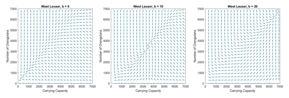
Figure 1: West Leuser.
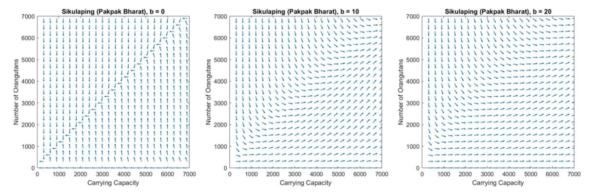
Figure 2: Sikulaping (Pakpak Bharat).
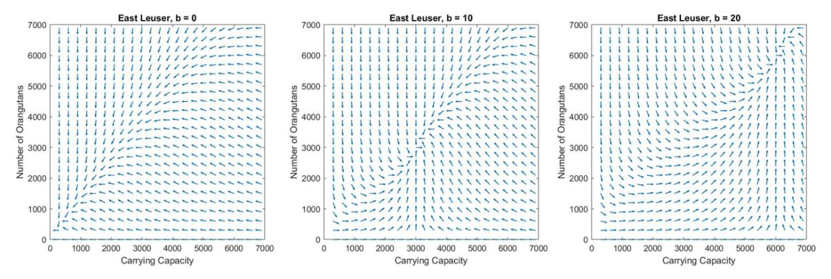
Figure 3: East Leuser.
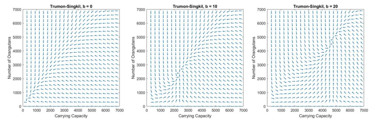
Figure 4: Trumon-Singkil.
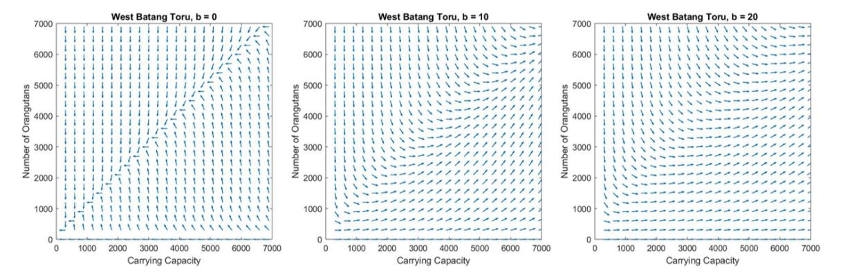
Figure 5: West Batang Toru.
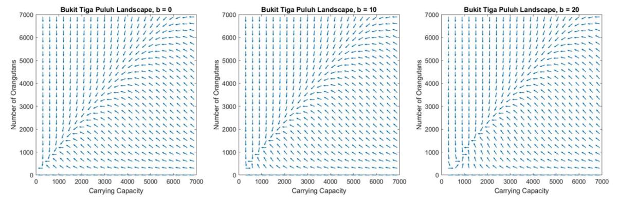
Figure 6: Bukit Tiga Puluh Landscape.
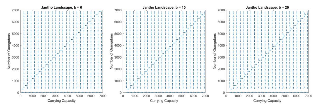
Figure 7: Jantho Landscape.
In accordance with what has been explained in the analysis model, the phase portrait in each area of Figure 1 - 7 will move towards the equilibrium point \((N_2, K_2) = (\frac{b}{s}, \frac{b}{s})\). The set of equilibrium points (N, K) in each area is given by Table 2.
Table 2: Equilibrium points (N, K) in each area.
| Area | \(N = K \ (b = 0)\) | \[N=K\ (b=10)\] | \(N=K\ (b=20)\) |
|---|---|---|---|
| West Leuser | 0 | 3,448.276 | 6,896.552 |
| Sikulaping (Pakpak Bharat) | 0 | 100,000 | 200,000 |
| East Leuser | 0 | 3,030.303 | 6,060.606 |
| Trumon-Singkil | 0 | 2,325.581 | 4,651.163 |
| West Batang Toru | 0 | 33,333.333 | 66,666.667 |
| Bukit Tiga Puluh Landscape | 0 | 529.101 | 1,058.201 |
| Jantho Landscape | 0 | 1,000,000 | 2,000,000 |
In Figure 1-7, almost the same interpretation results are obtained. In Figure 1 - 7, the simulation is run based on the parameter values in Table 1. From the numerical simulation results, it is found that the system being analyzed is stable at the equilibrium point \((N_2, K_2)\). Furthermore, it was also found that the orangutan population was greatly influenced by the carrying capacity, as seen from the simulation results where when b=0, the orangutan population was 0 or extinct. This indicates that when the orangutan habitat does not
exist, the orangutan will become extinct. So at \(b \neq 0\), it was found that orangutans would not experience extinction so the presence of habitat greatly affected the number of orangutan populations. In addition, from Figure 1-7 it is found that the higher the value of b, the higher the orangutan population. So based on the simulation, it is found that the wider the orangutan habitat, the higher the orangutan population. Meanwhile, if the area of their habitat is not increased, orangutans will experience extinction in every area.
The Sikulaping (Pakpak Bharat), West Batang Toru, and Jantho Landscape areas have orangutan populations that are relatively safe if carrying capacity is added constantly, at least with an b = 10.
We also perform simulations as if the rate of decline in forest loss changes periodically up and down. The highest decrease is assumed to be 2 times higher than the previous value of s but immediately followed by public action and government action (e.g. by making stricter regulations related to forest sustainability) so that the value of s continues to decline until there is no decrease in forest capacity. And when the value of s reaches 0, the rules are relaxed so that the value of s increases until it reaches back to 2 times higher than the previous value of s, and so on.
Therefore, we make modifications to the model to be:
\[\frac{dN}{dt} = \begin{cases} (r - \frac{q}{N_0})N(1 - \frac{N}{K}), & r > \frac{q}{N_0} \\ (r - \frac{q}{N_0})N, & r \le \frac{q}{N_0} \end{cases}, \tag{8}\]
\[\frac{dK}{dt} = -s(\cos\omega t + 1)K + b , r > \frac{q}{N_0}.\] (9)
We give a value \(\omega=1\). The \(\cos\omega t+1\) values are between 0 and 2. Especially for the Tripa Swamp, Siranggas/Batu Ardan, and East Batang Toru (Sarulla) areas which have a value of \(r-\frac{q}{N_0}<0\), the model used is the exponential model without changing the carrying capacity value (Figure 15). The following are the simulation results for each area:
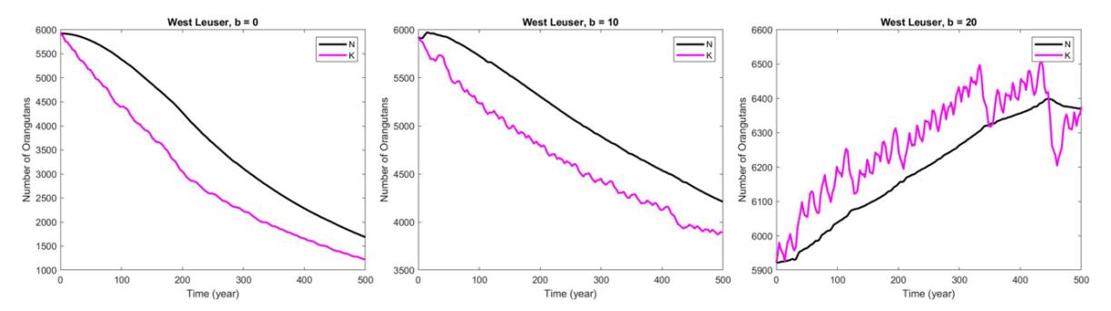
Figure 8: West Leuser.
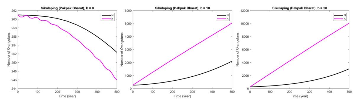
Figure 9: Sikulaping (Pakpak Bharat).
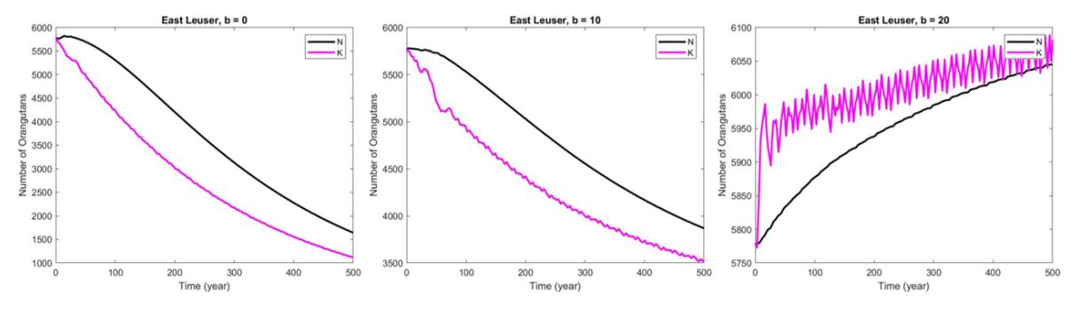
Figure 10: East Leuser.
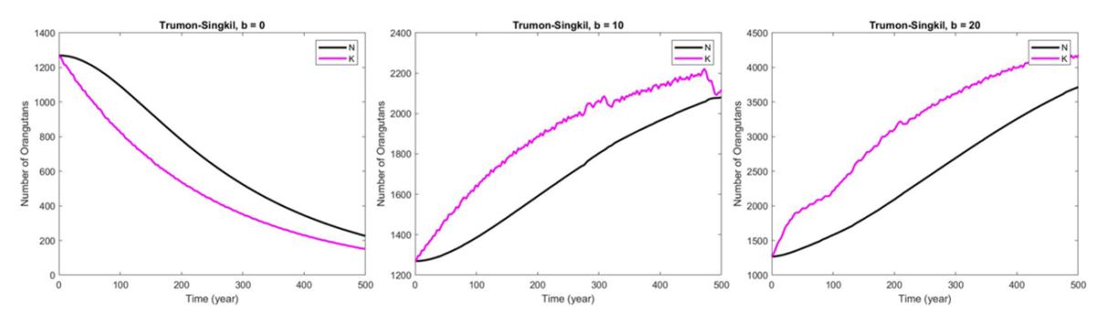
Figure 11: Trumon-Singkil.
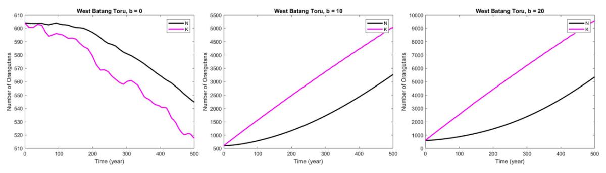
Figure 12: West Batang Toru.
According to the graph, it can be seen that the addition of carrying capacity is effective in areas that have a positive rate of increase in the orangutan population \((r>\frac{q}{N_0})\), shown in Figure 8 - 14. In all areas, for b=0, there is no attempt to increase carrying capacity, Orangutan population will continue to decline for at least the next 500 years. For the seven areas that are shown in Figure 8 - 14 with \(r>\frac{q}{N_0}\) and b=10, some areas have experienced a decline in orangutan population, but there is no area where the orangutan population decline is more than 50%. On the other hand, for b=20 which means that there is a sufficient effort to increase the carrying capacity, the orangutan population level has relatively increased in a period of 500 years.
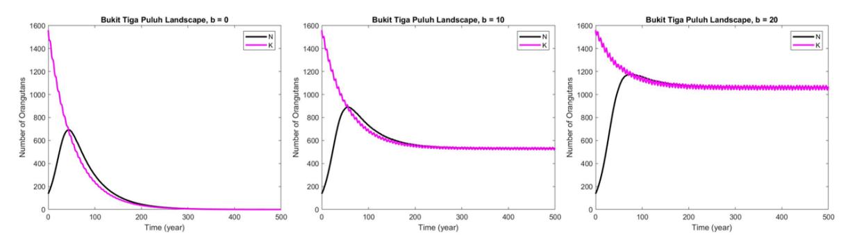
Figure 13: Bukit Tiga Puluh Landscape.
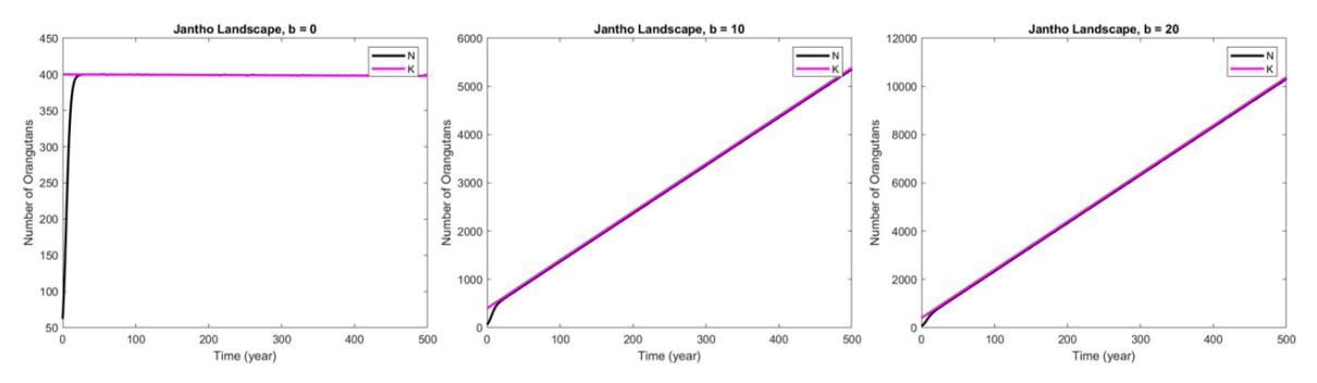
Figure 14: Jantho Landscape.
We can see in Figure 8 and 10 the value of carrying capacity is higher than the population when b = 20 for 500 years. Meanwhile, in Figure 9, 11, and 12 the value of carrying capacity is higher than population when b = 10 and b = 20 for 500 years. It means, addition to the value of b will change the value of carrying capacity in Figure 9, 11, and 12 more than the value of carrying capacity in Figure 8 and 10. Moreover, we can see that the characteristics for systems of differential equation for Figure 8 - 14 is that the value of N has the tendency to approach the value of K over the time. Figure 15 basically is just the picture of the curve N(t) = N0 exp[(r − q N0 )t]. It means, Figure 15 can be interpreted as the reduction of N exponentially.
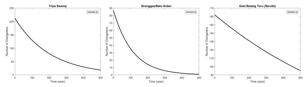
Figure 15: Tripa Swamp, Siranggas, East Batang Toru.
We conclude that the addition of carrying capacity is very necessary to save the orangutan population. However, in the Jantho landscape (Figure 14), if the rate of re-introduction is maintained, the decline in the orangutan population will be very slow, even without additional carrying capacity. However, the orangutan population will be stuck at carrying capacity, so the additional carrying capacity is still needed to increase the number of orangutans that can survive in the Jantho Landscape.
Based on reference [14], at b = 0 the only areas that meet the Minimum Viable Population criteria for Sumatran orangutans, namely the probability of extinction at 500 years < 10%, are only Sikulaping (Pakpak Bharat), West Batang Toru, and Jantho Landscape (Figure 9, 12, 14).
5. REDUCTION OF THE ORANGUTAN POPULATION
We observe that if b < 10, certain areas will experience a decline in the orangutan population by more than 50% from N0. Table 3 shows how many years it will take for the orangutan population decline to reach more than 50% in year t for b = 0, 2, and 9. The areas that are mathematically unlikely to experience a decline in orangutan population by more than 50% will be substituted an "x".
| Table 3: Time (years) required for the orangutan population to decrease by 50% from N0. |
|---|
| Area | t (b = 0) | t (b = 2) | t (b = 9) |
|---|---|---|---|
| West Leuser | 342 | 398 | x |
| Sikulaping (Pakpak Bharat) | 7,088 | x | x |
| East Leuser | 321 | 367 | 1,068 |
| Tripa Swamp | 142 | 142 | 142 |
| Trumon-Singkil | 252 | 488 | x |
| Siranggas/Batu Ardan | 77 | 77 | 77 |
| West Batang Toru | 2,439 | x | x |
| East Batang Toru (Sarulla) | 655 | 655 | 655 |
| Bukit Tiga Puluh Landscape | 178 | x | x |
| Jantho Landscape | 255,704 | x | x |
The following is a map visualization from table 3 using ArcGis:
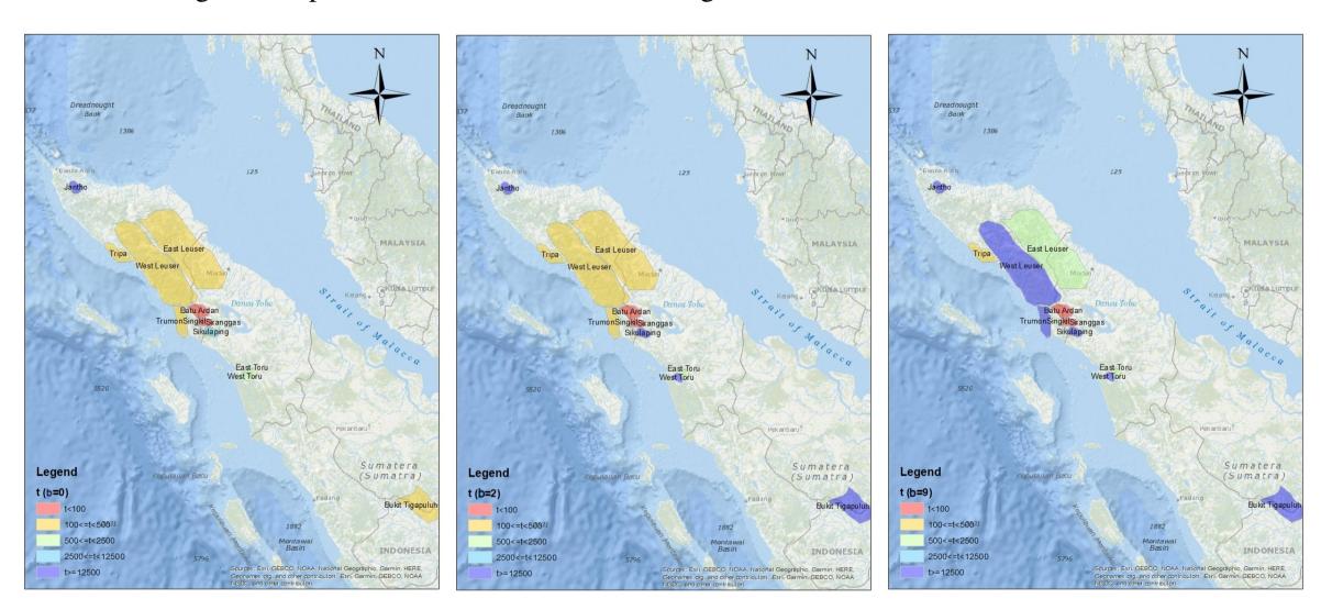
Figure 16: Pongo abelii habitat based on time (years) required to decrease by 50% from N0.
It seems from Figure 16 that for b = 0, yellow dominates the map, indicating that the orangutan population will decline by half from its initial value in about 100 and 500 years. For b = 2, the purple color has started to appear a lot so it can be said that there is a significant difference to b = 0, while at b = 9, the purple color already dominates the map so it can be said that the condition of the orangutans is quite safe in most areas for at least up to the next 500 years.
6. CONCLUSION
Based on the results of research, it is obtained that the orangutan population is strongly influenced by the availability of its habitat. The larger the habitat area, the higher the orangutan population. Meanwhile, if the habitat is not available, the orangutan will become extinct. So the results of this study can be used as a consideration for determining policies to maintain an increasingly extinct orangutan population. For the Tripa Swamp, Siranggas/Batu Ardan, and East Batang Toru (Sarulla) areas, another way is needed to maintain the orangutan population, namely by suppressing the q parameter which consists of poaching as trade, conflict killing, hunting/food, wounding, and fire. The value of q must be reduced to a minimum so that q < rN0. However, this research is still very limited due to the assumptions used and the limitations of the parameters used. For example, the value of the growth rate that we use are the same in each area. The simulation results of the orangutan population displayed in this study also differ from those listed by reference [14]. This is possible because of the difference between the mathematical model and the parameter values used.
ACKNOWLEDGEMENT
The authors would like to thank the Balai Konservasi Sumber Daya Alam (Nature Conservation Agency; Indonesia) team for providing some information. We also thank the organizers of the Ganesha Talent Assistantship (GTA) scholarship given to Karsten Maynard Jabriel and Muhamad Jamaludin while studying at Bandung Institute of Technology.