

1. Introduction
Dengue fever and dengue hemorrhagic fever are vector-borne diseases that are the leading causes the illness in many tropical and subtropical countries. According to World Health Organization, an estimated 50 million people worldwide are infected by dengue annually with a significant number (approximately 90%) of them being children aged less than five years old and about 2,5% of that infected die due to the dengue [1]. Dengue virus enters to host body when an infected female Aedes aegypti mosquitoes suck the blood of the targeted susceptible host and transmit the infection. Once the human had been bitten by the infected vector, they potentially spread the infection in the next blood meal of the mosquito. The mosquito becomes infected after biting infected humans and gains the capacity to spread the viruses [2]. Moreover, the biting rate plays an important role to spread the infection both in the host and vector populations.
Currently, there are numerous methods to reduce and control dengue transmission. The researchers [3] argued that controlling the mosquito population is still less effective in reducing disease transmission. The authors argued that the climate change variables should also be included in the model. Meanwhile, according to other researchers [4], the dengue vaccine is also necessary to prevent and implement vector control. The dengue outbreaks will continue as long as susceptible mosquitoes are still present. Suandi et al. [5] revealed that continuous usage of insecticide in dengue control has decreased its viability due to the emergence of resistant mosquitoes. In addition, Recker et al. [6] also argued that safe and effective vector control is a successful key to reducing dengue mortality and morbidity. Accordingly, Brand et al. [7] highlighted the importance of the distribution of times between life-history events through the length of the vector life cycle, which determines the time between successful bites.
Traditional vector control has less effective in reducing the spread of dengue in the population. For example in western Kenya uses edible fish of Larvivorous Oreochromis niloticus L to reduce the number of mosquito populations at the egg and larvae levels [8]. Exposure to silver nanoparticles that have been synthesized has also been used as a mosquito population control technique [9], [10], [11]. Another treatment for suppressing dengue transmission is using Wolbachia. It offers two mechanisms in order to reduce dengue which are a reduction in mosquito population density and bring down vector competence. Wolbachia is vertically transmitted through intracellular bacteria that are naturally among 60% of insects [12]. Furthermore, Wolbachia presents the potential strategy of biocontrol for arboviral disease including dengue [13].
There are some genetic modifications of using Wolbachia such as transgenic traits as population replacement in vector population [14] and pathogen-blocking phenotype. These genetic strategies are considered as an environmentally friendly strategy to replace the target population for controlling arboviral disease [15]. In this paper, the approach taken is to construct a genetic population model that describes mosquito population dynamics by involving random mating between mosquito populations with and without Wolbachia bacteria.
In this paper, the Wolbachia mosquito dynamics model will be constructed which is then analyzed by the behavior of the solution. After the introduction to explain the motivation of the dynamic model, the next section described how the model was constructed. This section is explained in detail how the transmission of wolbachia bacteria through the mechanism of the Mandel rules then the model is constructed. In the third section, the stability analysis of the equilibrium point that has been obtained is presented in detail. In the fourth section, numerical simulations are presented as confirmation of the results of the previous stability analysis. In the numerical simulation section, the behavior of the solutions of the model that has been constructed is analyzed. In addition, the sensitivity of the parameters to changes in solutions behavior is explored. Finally, a conclusion is presented that summarizes the results of this study.
2. MATHEMATICAL MODEL
Insufficient reference to mathematical modeling that describes the spread of vector-borne diseases involving control factors through Wolbachia genetic modification is one of the main reasons for constructing this model. This model is expected to be a basic description in constructing more complex mathematical models because this model will focus only on the population development of Wolbachia-infected mosquitoes. Based on the results of research [16], [17], [18], there are at least three interesting phenomena that can be observed from the Wolbachia-infected mosquito population, namely: the ability of the Wolbachia-infected female population to survive and reproduce in the absence of a male population, infected male mosquitoes can grow well as fertile or infertile females (feminization), the presence of cytoplasmic incompatibility, namely the inability of female mosquito populations to produce offspring when mating with Wolbachia-infected male mosquitoes. The last phenomenon, namely cytoplasmic incompatibility, is the main focus in the construction of this model. In addition, the population is assumed to be isolated and the population size is not constant. In contrast to the model proposed by Yazhi Li and Xianning Liu in [19], this paper will describe the construction of a model that explicitly involves mating rules. The mating rule to be adopted is random mating, i.e. individuals mate according to the rule of probability products. This is more realistic in large populations and assumes that the trait studied does not affect reproduction. Finally, it is also assumed that the population of Wolbachia-infected mosquitoes is already present in the reproductive area.
2.1. Wolbachia Bacteria Transmission Mechanism
Let's say SS is the genotype of wild-type mosquitoes and produces S gametes. Meanwhile, WW is the genotype of mosquitoes infected with Wolbachia and produces W gametes. In the F2 generation, Wolbachia bacteria can be passed on to the next generation by the Mendelian rule mechanism described in Table 1.
Table 1 demonstrates the mechanism of inheritance of the Wolbachia bacterial allele from the parent generation to the next generation. The population of female SS mosquitoes that produce the S allele gives birth to mosquitoes with the SS genotype when mating with male mosquitoes with the SS genotype, but will not give birth to offspring when mated with male mosquitoes with the WW genotype due to cytoplasmic incompatibility resulting in premature embryo death. Meanwhile, female mosquitoes with genotype WW that produce W gametes will give birth to a population of mosquitoes carrying Wolbachia bacteria SW (heterozygote) when mating with male mosquitoes with genotype SS and give birth to mosquitoes with genotype WW when mating with mosquitoes infected with Wolbachia.
| ♂× ♀ | SS | WW | |
|---|---|---|---|
| S | W | ||
| SS | S | SS | SW |
| WW | W | ∅ | WW |
Table 1: Punnett square to describe the possibility for a mechanism of Wolbachia bacterial transmission.
2.2. Mathematical Model Construction
Suppose u(t) and v(t) are the number of S and W alleles in the gene pool, respectively, each time t. Meanwhile, n(t) is the total gene in the gene pool for each time t. The growth rates of alleles and total alleles in a gene pool are determined by Equation (1),
\[u' = m_1 u; \ v' = m_2 u; \ \text{and} \ n' = \bar{m}n;\] (1)
where m1, m2 are Malthusian parameters for the growth of S and W alleles respectively. Meanwhile, m¯ is the average allele growth rate in the gene pool. Consider
\[x = -\frac{u}{n}; \ y = -\frac{v}{n} \tag{2}\] are the proportions of the S allele and the W allele, respectively. Take the derivative to Equation (1) yields
\[x' = \left(\frac{u}{n}\right)'\] \[= \frac{u'n - n'u}{n^2}\] \[= x \left(m_1 - \bar{m}\right).\] (3)
Similar way will give y ′ = y(m2 − m¯ ). Next, to obtain the magnitudes of m1, m2 and m¯ , consider the frequency changes of each gamete before and after selection in Table 2.
Table 2: Genotypic and gamete frequency of mosquitoes before and after selection.
| Frequency | Gamete | ||||
|---|---|---|---|---|---|
| Genotype | Before selection | After selection | S | W | |
| S × S | 2 x | αx2 | 1 | 0 | |
| S × W | xy | ηxy | 1 2 | 1 2 | |
| W × W | 2 y | γy2 | 0 | 1 | |
Table 2 indicate there is a fitness factor (α, η, γ) for each genotype (SS, SW, WW) after going through the selection factor. It should be noted in this model that the maximum value of the fitness level of each genotype is one, namely 0 < α, η, γ < 1. The magnitude of m1 is obtained by adding up the product of column 3 (column frequency after selection) and column 4 in Table 2 so as to give the probability of parents producing gametes S divided by x. Meanwhile, m2 is obtained by adding up the product of column 3 and column 5 which contains the probability of producing gametes W then divided by y. Mathematically, the Malthusian parameters of each of the S and W alleles are determined respectively in Equation 4.
\[m_{1} = \frac{\alpha x^{2} + (1/2)\eta xy}{x} = \alpha x + \frac{\eta}{2}y,\] \[m_{2} = \frac{\gamma y^{2} + (1/2)\eta xy}{y} = \gamma y + \frac{\eta}{2}x.\] (4)
As a result, a mathematical model that describes the population dynamics of Wolbachia-infected mosquitoes is formulated in Equation (5).
\[x' = x \left[ \left( \alpha x + \frac{\eta}{2} y \right) - \bar{m} \right],\] \[y' = y \left[ \left( \gamma y + \frac{\eta}{2} x \right) - \bar{m} \right],\] (5)
where average of allele growth rate \(\bar{m} = \alpha x^2 + \eta xy + \gamma y^2\) which is obtained by adding up all the third columns in Table 2. The solution of the differential equations system (5) is a solution that remains positive for the future time when a positive initial value is given. This argument can be verified by applying the dot product operation to the vector field and the normal vector evaluated at the boundary. The dot product of Equation (5) and the normal vector for \(R^2\) space is the following equation:
\[\begin{pmatrix} x' \\ y' \end{pmatrix} \cdot \begin{pmatrix} 1 \\ 0 \end{pmatrix} \bigg|_{x=0} = x' \bigg|_{x=0} = 0, \text{ and } \begin{pmatrix} x' \\ y' \end{pmatrix} \cdot \begin{pmatrix} 0 \\ 1 \end{pmatrix} \bigg|_{y=0} = y' \bigg|_{y=0} = 0.\]
These results indicate that when the solution orbit of Ssystem (5) strikes the boundary it will remain in the first quadrant. Moreover, it can be shown that System (5) has a bounded solution. To prove this statement, suppose N = x + y. Consider that,
\[\frac{dN}{dt} = \bar{m}(1 - N) \leq \max\{\alpha, \eta/2, \gamma\} N^2 (1 - N) \leq N^2 (1 - N).\] (6)
Equation (6) leads to the final result \(\limsup N(t) = 1\) for t to infinity. Therefore, all solutions of x and y are bounded by one. As a result, the system of differential equation (5) is mathematically and biologically well-defined.
3. STABILITY OF EQUALIBRIA
By solving the system (5) when x' = y' = 0, four equilibria are found where three equilibria are in the boundary and one interior equilibrium. From the inside of the three equilibria at the boundary, there is one population extinction equilibrium \(\mathcal{E}_0(0,0)\) which is always unconditionally unstable so further discussion of this equilibrium is uneventful and has no significant biological interpretation. Meanwhile, the two boundary equilibria and one interior equilibrium are as follows:
\(\mathscr{E}_1 := (1,0)\) represent the monomorphic of wild type equilibrium,
\(\mathscr{E}_2 := (0,1)\) represent the monomorphic of Wolbachia-infected equilibrium,
\[\mathscr{E}_3 := \left(\frac{\eta - 2\gamma}{2(\eta - \alpha - \gamma)}, \frac{\eta - 2\alpha}{2(\eta - \alpha - \gamma)}\right) \quad \text{represent the polymorphic equilibrium}.\]
Monomorphic equilibrium stability shows the natural characteristics of the population, namely the high level of survival (fitness level) of a group can lead to conditions where the group dominates the population.
This fact is supported by the eigenvalues of the Jacobian matrix which are evaluated at the corresponding monomorphic equilibrium respectively {−α, η/2−α} and {−γ, η/2−γ}. The stability of the monomorphic equilibrium E1 and E2 respectively depends on the fitness level of each subpopulation, α > η/2 and γ > η/2. It is clearly indicated that the level of dominance of a particular species group in the population is based on its fitness level. In fact, when α > η/2 > γ then the solution orbit of the system (5) converges to equilibrium E1 of any positive initial value. On the other hand, when γ > η/2 > α then the solution orbit of the system (5) converges to equilibrium E2. This result will be confirmed again in the numerical simulation.
The existence of polymorphic equilibrium E3 depends on the fitness of SW genotype as a carrier of the Wolbachia-infected gene, namely when η > 2 max{α, γ} or η < 2 min{α, γ}. In case η > 2 max{α, γ}, it is easy to verify that both the numerator and denominator of the equilibrium E3 are positive. Meanwhile, if η < 2 min{α, γ} the numerator and denominator of equilibrium E3 are negative. As a result, these two conditions accompany the equilibrium E3 to the interior of the first quadrant. Next, consider second-order polynomials (7) to investigate the stability of polymorphic equilibrium,
\[\underbrace{16(\alpha + \gamma - \eta)^2}_{:=A} \lambda^2 + \underbrace{8\eta(\alpha + \gamma - \eta)^2}_{:=B} \lambda + \underbrace{(\eta - 2\gamma)(\eta - 2\alpha)(\eta^2 - 4\alpha\gamma)}_{:=C} = 0. \tag{7}\]
Equation (7) is a polynomial characteristic of the Jacobian matrix which is evaluated at polymorphic equilibrium E3. It is easy to notice that A and B from Equation (7) are positive. Hence, the stability of the polymorphic equilibrium E3 is determined by the sign on C. The part of C in Equation (7) is positive if η > 2 max{α, γ}. This indicates that the two roots of Polynomial (7) have the same sign and both are negative. As a result the polymorphic equilibrium E3 is locally asymptotically stable. However, if η < 2 min{α, γ} we can obviously establish that η 2 − 4αγ is negative, consequently that C is negative. This leads to a situation where the roots of Polynomial (7) are real and have different signs, consequently the polymorphic equilibrium E3 is an unstable saddle. If the stability situation of the three equilibria is depicted as a whole on a parameter diagram, then four regions will be obtained with different gene pool characteristics as shown in Figure 1.
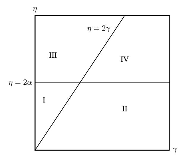
Figure 1: Parameter space that shows the region of equilibria stability: (I) E1 stable; E2 unstable; (II) E1 and E2 stable but E3 unstable; (III) E1 and E2 unstable but E3 stable; (IV) E1 unstable; E2 stable.
Region I is a condition where the fitness level α > η/2. As previously discussed, the results of the stability analysis show that in this region the monomorphic of wild-type equilibrium E1 is stable while the monomorphic of Wolbachia-infected equilibrium E2 is unstable. In this region, the polymorphic equilibrium E3 does not exist. This situation is also known as directional selection on susceptible. The polymorphic equilibrium E3 exists in region II but is unstable. In this region, under dominance behavior occurs where double stability occurs from both equilibrium at the boundary, i.e. E1 and E2. The convergence of the solution
orbits will depend on their initial values. The stability of the polymorphic equilibrium E3 attended by the instability of the two monomorphic equilibria can be established in region III. This circumstance is also notable as the overdominance behavior of the population. In region IV, the polymorphic equilibrium E3 again did not exist and was recognized by the stability of the monomorphic Wolbachia-infected equilibrium E. The terms for the population dominance circumstances from Model (5) are summarized in Table 3.
| Condition | Description |
|---|---|
| η > 2 max{α, γ} | overdominance |
| η < 2 min{α, γ} | underdominance |
| α > η/2 > γ | directional selection on susceptible |
Table 3: Dominance-related conditions for the dynamic Model (5).
4. NUMERICAL SIMULATION
γ > η/2 > α directional selection on Wolbachia-infected
In this section, the perform a numerical simulation is presented to confirm the analytical results. The numerical data used for this simulation is selected randomly so that it can represent four regions in Figure 1 whose conditions are adjusted to the terms in Table 3. The data is shown in Table 4. This numerical simulation consists of two parts. The first is a simulation to determine the dynamic behavior of the model by drawing the orbital solution of the model (5). In the second stage, the simulation is carried out to determine the sensitivity of a parameter to changes in dynamic behavior. Runge Kutta method of order 4 is used to determine the solution of model (5).
| Parameters | Region | |||
|---|---|---|---|---|
| I | II | III | IV | |
| α | 0.35 | 0.3 | 0.2 | 0.2 |
| η | 0.6 | 0.5 | 0.9 | 0.6 |
| γ | 0.2 | 0.4 | 0.3 | 0.35 |
Table 4: Parameter values for simulation in each region.
4.1. Dynamic Behavior
By solving Equation (5) using the parameter values in Table 4, a phase portrait can be described for each region as shown in Figure 2. Figure 2(a) represents the dynamic behavior in region I where the heterozygote fitness level is smaller than twice the monomorphic susceptible fitness. In addition, the fitness of monomorphic wolbachia is smaller than other fitness. This condition leads to the failure of the Wolbachia bacteria invasion where the susceptible S allele dominates the gene pool. As a result, the population will be dominated by mosquitoes with the SS genotype. This situation is also known as directional selection on susceptible. A very different behavior occurred in region IV where the fitness level of Wolbachia-infected mosquitoes dominated other fitness levels, even exceeding half of the heterozygous fitness level. This situation leads to the successful invasion of Wolbachia-infected mosquitoes where the gene pool will be dominated by the W allele so that Wolbachia-infected mosquitoes dominate the population (see Figure 2(b)). Under these two conditions, polymorphic equilibrium does not exist. The polymorphic equilibrium only exists when the heterozygous fitness value is at an extreme (maximum or minimum) condition. In the condition that the heterozygous fitness level is greater than twice the monomorphic fitness level, the polymorphic equilibrium exists and is stable. This condition is known as overdominance where wild-type mosquitoes and Wolbachiainfected mosquitoes can coexist. The solution orbit of System (5) converges to interior equilibrium as in Figure 2(c). However, when the half heterozygous fitness level is at its lowest value then the solution orbits converge to an equilibrium point at the boundary. In this condition, there are two equilibria at the stable limit while the interior equilibrium is unstable. The behavior of this solution also confirms that the initial proportion of the population greatly influences the state of the final population in the gene pool. This situation is known as under dominance, where the level of dominance of the final population depends on the proportion of the initial population (see Figure 2(d)).
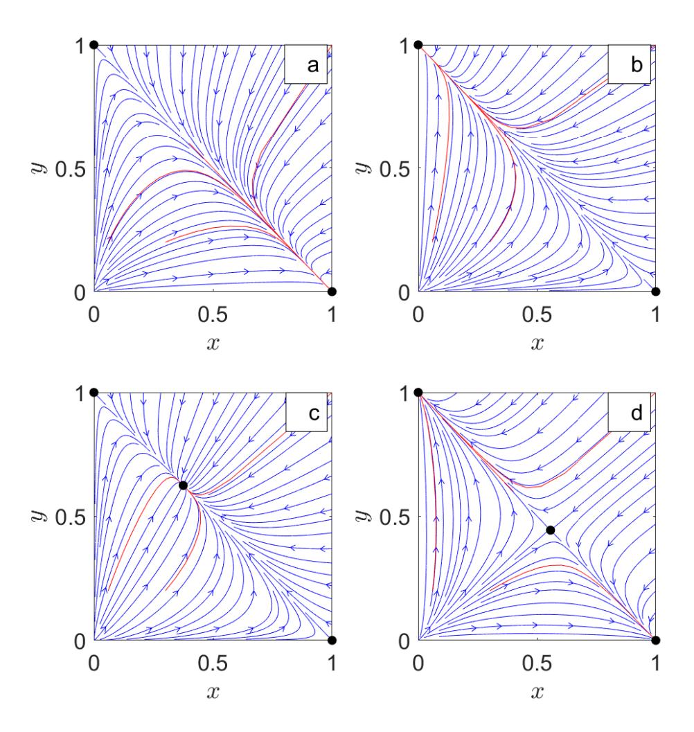
Figure 2: Phase portrait for model (5) of each stability region with parameter values in Table 4.
4.2. Sensitivity Analysis
In addition to equilibrium stability analysis, qualitative behavior analysis can also be carried out through sensitivity analysis. This technique can provide information about the effect of parameter changes on variables from time to time. It also allows us to investigate the parameters that have the most effect on changes in the behavior of the variables. This technique has been used in many kinds of literature such as in [20], [21], [5]. Suppose set of parameter \(\theta = \{\alpha, \eta, \gamma\}\) and variables \(\mathbf{X} = \{x, y\}\) is the solution of \(\partial_t \mathbf{X} = \mathbf{F}(\mathbf{X}, \theta)\) where \(\mathbf{F} = \{f_1, f_2\}\) is the right hand side of the model (5). Define the regulatory function for sensitivity \(S = \partial \mathbf{X}/\partial \theta\). The derivative of sensitivity function respect to time t is
\[\frac{dS}{dt} = \frac{d}{dt}\frac{\partial \mathbf{X}}{\partial \theta} = \frac{\partial}{\partial \theta}\frac{d\mathbf{X}}{dt} = \frac{\partial}{\partial \theta}\mathbf{F}(\mathbf{X}, \theta) = \frac{\partial \mathbf{F}}{\partial \mathbf{X}}\frac{\partial \mathbf{X}}{\partial \theta} + \frac{\partial \mathbf{F}}{\partial \theta}.\] (8)
From Equations (8), the expression of \(\partial F/\partial X\) is a Jacobian matrix with ordo \(2\times 2\) of the model (5). The data used to perform sensitivity analysis is data where the polymorphic equilibrium point exists with stable or unstable conditions. The simulation results from the sensitivity analysis which is the solution of system (8) using the Runge Kutta method is shown in Figure 3. The results of the sensitivity analysis when the polymorphic equilibrium is stable are shown in Figure 3(a) – (b).
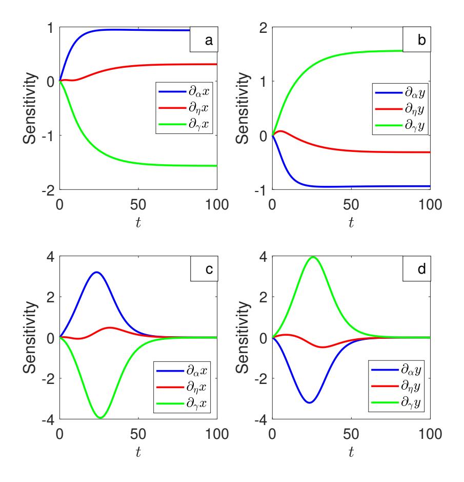
Figure 3: Sensitivity analysis over time for both compartments x and y with parameter conditions: (a)-(b) stable polymorphic equilibrium; (c)-(d) unstable polymorphic equilibrium.
In Figure 3(a), the parameter that dominates the behavior change of x is the fitness level of Wolbachiainfected γ with a negative effect. This shows that the greater the fitness of Wolbachia-infected mosquitoes, the lower the proportion of the wild-type mosquito population. Furthermore, the fitness level of wild-type mosquitoes, α is at the second level which has the most influence on changes in the wild-type mosquito population. The greater the survival rate of the wild-type mosquito population, the greater the proportion of the wild-type mosquito population in the gene pool. Meanwhile, the proportion of Wolbachia-infected mosquitoes may decrease when the fitness level of wild-type mosquitoes increases (see Figure 3(b)). From the three parameters involved, the fitness level of Wolbachia-infected mosquitoes has a higher effect on changes in the proportion of mosquito populations, whether Wolbachia-infected mosquitoes or wild-type mosquitoes. It's just that the effect is different, namely a positive impact for the population of mosquitoes infected with Wolbachia and a negative for the population of wild-type mosquitoes. This condition is also maintained when the polymorphic equilibrium is unstable. The fitness level of the heterozygous mosquito population, η did not have a significant impact on the two types of mosquito population, both in stable and unstable polymorphic states (see Figure 3).
5. CONCLUSION
A mathematical model describing the population dynamics of Wolbachia-infected mosquitoes has been constructed. The results of the analysis show that there are three equilibrium points, each of which represents the condition of monomorphic of wild-type, monomorphic of Wolbachia-infected and polymorphic equilibrium. The stability of the three equilibria was analyzed locally so as to obtain information about the qualitative behavior of the mosquito population. The existence of alleles in the gene pool of mosquito populations depends on the level of their fitness in nature. When the fitness level of wild-type mosquitoes is higher than the others, the alleles of wild-type mosquitoes dominate the gene pool. Consequently, the proportion of wild-type mosquito populations is higher than the population of Wolbachia-infected mosquitoes. This condition also provides extinction potential for Wolbachia-infected mosquitoes. The behavior is different when the fitness level of mosquitoes infected with Wolbachia is higher than others. This condition causes the population of mosquitoes infected with Wolbachia to be dominant in the population and even the wild-type mosquito population is indicated to be extinct. This happens because the gene pool is dominated by alleles infected with Wolbachia. However, if heterozygous mosquitoes has a fitness level two times greater than the fitness level of homozygous mosquitoes, the two sub-populations of mosquitoes are co-existence. Furthermore, from the results of the sensitivity analysis, there is a strong suspicion that the fitness level of the population of Wolbachia-infected mosquitoes has an important role in population dynamics and allow to suppresses the proportion of wild-type mosquito populations. This shows that the injection of Wolbachia bacteria has a positive effect on the expansion of Wolbachia-infected mosquitoes. Some interesting phenomena from the effect of Wolbachia mosquito development on controlling cases of disease spread caused by mosquito vectors have not been observed as a whole. In future studies, factors such as the reproductive ability of female Wolbachia mosquitoes in the absence of male mosquitoes need to be investigated in order to obtain a comprehensive understanding.