

1. INTRODUCTION
The story of COVID-19 is not yet complete. After successfully maintaining an essentially disease-free status for almost two years, China is once again implementing lockdowns, following the unprecedented omicron outbreak, which is mentioned to be "ten times more severe" than the original Wuhan outbreak in 2020 [30]. Indeed, the country's previously-unchanging maximum number of daily new cases, 15,133, recorded on 13 February 2020, was surpassed on 5 April 2022 with 16,649 new cases, before the latest maximum of 53,345 new cases was reported on 15 April 2022 [14].
The scientific impact of COVID-19 has been remarkable. Over the last three years, the literature has witnessed a surge of interest in the study of the disease's spread, particularly via mathematical models [18], [12], [1], [31], [23], [11], [10], [21], [6], [2], [3], [5], [20], [24], [7], [25], [22]. Indeed, while the classic SIR-type disease-spread model of Kermack and McKendrick [15] incorporated merely the disease's intrinsic transmission and recovery rates, numerous mathematical models constructed to study the spread of COVID-19 have incorporated various extrinsic factors, such as the susceptible individuals' cautiousness level [5], [20], [24], [7], [25], a high value of which inhibits the disease's transmission rate, as well as the hospitals' bed-occupancy rate [6], [2], [3], a high value of which inhibits the disease's recovery rate.
In mid 2021, we initiated our study by developing the following simple, SIR-type model which incorporates as key parameters both the susceptible individuals' cautiousness level γ ∈ [0, 1] and the hospitals' bedoccupancy rate ρ ∈ [0, 1], as presented in Model 1.
∗Corresponding author
Received June 10th, 2023, Revised August 10th, 2023 (first), Revised August 28th, 2023 (second), Accepted for publication October 14th, 2023. Copyright ©2023 Published by Indonesian Biomathematical Society, e-ISSN: 2549-2896, DOI:10.5614/cbms.2023.6.2.6
| Parameter | Description | Unit |
|---|---|---|
| β | transmission rate | \[\frac{1}{\text{individual} \times \text{day}}\] |
| \(\lambda\) | entry rate | individual day |
| \(\mu\) | natural death rate | \(\frac{1}{\text{day}}\) |
| \(\mu'\) | death rate due to COVID-19 | \(\frac{1}{\text{day}}\) |
| \(\alpha\) | recovery rate | \(\frac{1}{\text{day}}\) |
| \(\rho\) | bed-occupancy rate | 1 individual |
| \(\gamma\) | cautiousness level | 1 individual |
Table 1: Parameters involved in the model (1).
\[\begin{cases} \frac{dS}{dt} = \lambda - \mu S - \frac{\beta SI}{1 + \gamma S}, \\ \frac{dI}{dt} = -\mu I - \mu' I + \frac{\beta SI}{1 + \gamma S} - \frac{\alpha I}{1 + \rho I}, \\ \frac{dR}{dt} = -\mu R + \frac{\alpha I}{1 + \rho I}, \end{cases} (1)\]
where S=S(t), I=I(t), and R=R(t) denote the sizes of the susceptible, infected, and recovered subpopulations at time \(t\geqslant 0\), while \(\beta,\lambda,\mu,\mu'\), and \(\alpha\) are positive parameters [27]. See Table 1. Subsequently, we applied the model (1) to the case of Jakarta, with the aim of constructing a quantitative method to determine the appropriate level(s) of social restrictions to be enforced in the region on any given day, based on the latest values of the bed-occupancy rate and the effective reproduction number [28]. Most recently, as the Indonesian government intensifies its eradicative effort through five forms of interventions: vaccinations, social restrictions, tracings, testings, and treatments, we proposed a substantial modification of the model which takes these into account, with the aim of identifying optimal intervention strategies [29].
From the analysis presented in [27], we have seen that the model (1), despite its simplicity, exhibits rich dynamical behaviour. Firstly, adding the model's three equations, one verifies that the total population is not constant. The stability analysis carried out in [27] have shown that the model possesses a unique disease-free equilibrium \(e_0 = (\lambda/\mu, 0, 0)\) for every set of parameter values, which is stable (unstable) if \(\mathcal{R}_0 < 1\) (\(\mathcal{R}_0 > 1\)), where
\[\mathcal{R}_{0} = \frac{\beta \lambda}{(\mu + \gamma \lambda) (\mu + \mu' + \alpha)},\tag{2}\]
is the model's basic reproduction number, as well as at most three positive endemic equilibria \(e_1\), \(e_2\), \(e_3\). Furthermore, fixing the parameter values
\[\beta = 0.05, \qquad \lambda = 10, \qquad \mu = 0.01, \qquad \mu' = 0.1, \qquad \alpha = 0.2,\] (3)
<sup>1</sup>These parameter values all originate from equation (8) in [27]. As explained therein, they are chosen not primarily to represent the epidemic situation in any geographical region, but to expose the model's rich dynamical behaviour. For a study of the same model using parameter values representing the actual situation in Jakarta (with \(\lambda\), \(\mu\), \(\mu\), \(\rho\) adopted from [4], [19] and \(\alpha\), \(\beta\) estimated using the L-BFGS-B algorithm [9]), see [28], where we constructed a design of governmental policies for the eradication of COVID-19 in the region.
ρ = 0.1 while letting γ vary over [0, 1], we observed that the model undergoes a number of codimension-one bifurcations: backward transcritical, Hopf, and saddle-node bifurcations of equilibria, as well as homoclinic and saddle-node bifurcations of limit cycles, the latter two being detected via numerical continuation, using AUTO. With regards to the model's codimension-two bifurcations, however, we have only pointed out without details in [27] that, by letting both γ and ρ vary over [0, 1], one finds instances of Bogdanov-Takens and generalised Hopf bifurcations. In the present paper, we shall continue the study of the model (1) by discussing these bifurcations in greater detail, along with their epidemiological implications.
The discussion is organised as follows. In the upcoming section 2, we establish a connection between what has been done in [27] and what is to be done in the present paper. We also describe the way in which we use AUTO to detect the aforementioned bifurcations, and give a brief summary of the topological changes occurring near each bifurcation point. In the subsequent section 3, we give a more detailed explanation on these changes and what they epidemiologically imply. Essentially, these changes can be viewed as complex manners in which the model's asymptotic behaviour transitions from endemic to disease-free, which involves the births and disappearances of limit cycles and homoclinic orbits, all occurring under the condition that R0 < 1 and that the model's transcritical bifurcation taking place at the basic reproduction threshold is backward. We also recommend several strategies for the disease's eradication which arise from our findings. In the final section 4, we summarise our conclusions and describe possible avenues for further investigation.
2. OVERVIEW
For the rest of the paper, we fix the values of β, λ, µ, µ ′ , and α as in (3). The basic reproduction number (2), being independent of ρ, reduces to a univariate function of γ:
\[\mathcal{R}_0 = \frac{5000}{31 + 31000\gamma}. (4)\]
Letting both γ and ρ vary over [0, 1], we have detected using AUTO [8] a set of bifurcation curves on the γρ-plane, each of which being a set of points (γ, ρ) on the unit square at which the model undergoes a specific bifurcation. In Figure 1, we display these curves in the region containing the richest discovered dynamical behaviour:
\[\left[\gamma_0, 0.42\right] \times \left[\rho_0, 0.27\right], \qquad \text{where} \qquad \gamma_0 := \frac{4969}{31000} \quad \text{and} \quad \rho_0 := \frac{29791}{100000000}.\]
As easily verified, in the entire region we have from (2) that R0 < 1, and from [27, Theorem 2.4] that the transcritical bifurcation at the basic reproduction threshold is backward. The region, therefore, consists of two adjacent subregions, in each of which the model possesses zero and two endemic equilibria, separated by a saddle-node bifurcation curve, containing points (γ, ρ) at which these equilibria coalesce. In Figure 1, this curve is plotted in blue, and is obtained by carrying out bidirectional continuation beginning from the saddle-node bifurcation point discussed in [27, section 3]:
\[\left(\gamma^{(\mathrm{SN})}, 0.1\right), \qquad \text{where} \qquad \gamma^{(\mathrm{SN})} \approx 0.356902.\]
The curve plotted in black, on the other hand, is a Hopf bifurcation curve, obtained similarly from the Hopf bifurcation point
\[\left(\gamma^{(\mathrm{HB})}, 0.1\right), \qquad \mathrm{where} \qquad \gamma^{(\mathrm{HB})} \approx 0.349638,\]
discussed in [27, section 3].
The Hopf curve has its endpoints lying on the saddle-node curve:
\[BT_1 \approx (0.404023, 0.229494) \qquad \text{ and } \qquad BT_2 \approx (0.164201, 0.002600) \,.\]
Letting γ and ρ vary smoothly so that the point (γ, ρ) travels anticlockwise around each BTi , one observes the following topological changes, to be detailed in the next section:
- (i) a homoclinic orbit emanates around a saddle endemic equilibrium via a homoclinic bifurcation, before shrinking and becoming an unstable limit cycle which surrounds a stable endemic equilibrium;
- (ii) the unstable limit cycle is absorbed by the stable endemic equilibrium, which then becomes unstable, via a Hopf bifurcation;
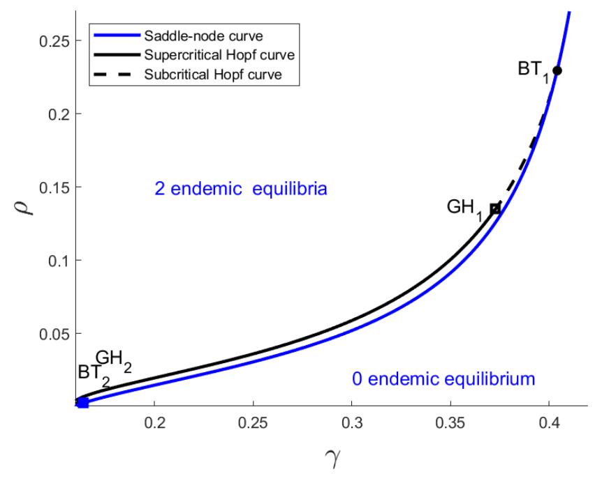
Figure 1: The codimension-two bifurcation diagram of the model (1) in the region [γ0, 0.42]×[ρ0, 0.27] on the γρ-plane, using the values of β, γ, µ, µ ′ , and α listed in (3).
(iii) the two equilibria coalesce and disappear via a saddle-node bifurcation.
Therefore, at each BTi , the model undergoes a Bogdanov-Takens bifurcation [16, section 8.4].
As also apparent in Figure 1, the Hopf curve consists of a solid supercritical Hopf curve, which indicates the ejection of a stable limit cycle, connected at its endpoints
\[GH_1 \approx (0.372814, 0.134955)\] and \(GH_2 \approx (0.163907, 0.002496)\), to two subcritical Hopf curves, which indicate the ejection of unstable limit cycles. As the point (γ, ρ) travels anticlockwise around each GHi , the following topological changes occur, again to be detailed in the next section:
- (i) a homoclinic orbit emanates around a saddle endemic equilibrium via a homoclinic bifurcation, before shrinking and becoming an unstable limit cycle which surrounds a stable endemic equilibrium;
- (ii) the stable endemic equilibrium loses stability while ejecting a stable limit cycle, via a Hopf bifurcation;
- (iii) the two limit cycles coalesce and disappear, via a saddle-node bifurcation of limit cycles.
Therefore, at each GHi , the model undergoes a generalized Hopf bifurcation [16, section 8.3].
We thus have four codimension-two bifurcation points of the model (1): BT1, BT2, GH1, and GH2. In the next section, we shall look at the neighbourhoods of these points, and describe the qualitatively different dynamical behaviours which may be possessed by the model's orbits for various pairs (γ, ρ) belonging to these neighbourhoods. From the perspective of epidemiology, these behaviours will confirm the significance of the bifurcation parameters γ and ρ for the eradication of COVID-19. The specific epidemiological implications will also be discussed, along with a number of concrete recommendations for the disease's eradication.
3. LOCAL BEHAVIOUR AND EPIDEMIOLOGICAL IMPLICATIONS
In this section, we visualise and describe the model's orbital behaviours at various points (γ, ρ) lying in the neighbourhoods of the four bifurcation points, and explain their epidemiological implications. In Figure 2, we display magnifications of Figure 1 in these neighbourhoods. In each neighbourhood, we shall choose
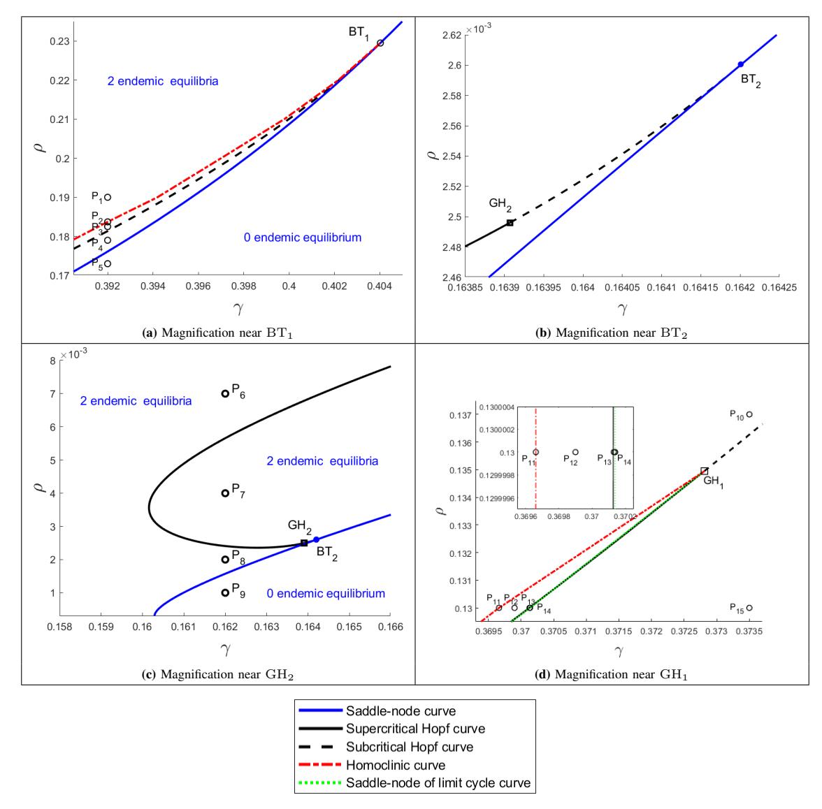
Figure 2: Magnifications of Figure 1 near the Bogdanov-Takens points BT1, BT2 and generalised Hopf bifurcation points GH1, GH2, with additions of homoclinic and saddle-node of limit cycle curves.
a number of specific points (γ, ρ) representing a number of qualitatively different orbital behaviours which indicate the occurrence of the respective bifurcation. These behaviours, which we now explain in detail, are all visualised in the model's three-dimensional phase portraits arranged in Figures 3 and 4. The corresponding two-dimensional phase portraits, obtained by projecting into the SI-plane the phase portraits in Figures 3 and 4, are presented in Appendices 1.1 and 1.2.
3.1. The dynamical behaviour near BT1
Figure 2 (a) shows a magnification of Figure 1 near the Bogdanov-Takens bifurcation point BT1, with the addition of a homoclinic bifurcation curve, plotted in red. Let us fix the susceptible individuals' cautiousness level at γ = 0.392, begin with a relatively high value of the hospitals' bed-occupancy rate ρ, and describe the topological changes occurring as ρ decreases gradually.
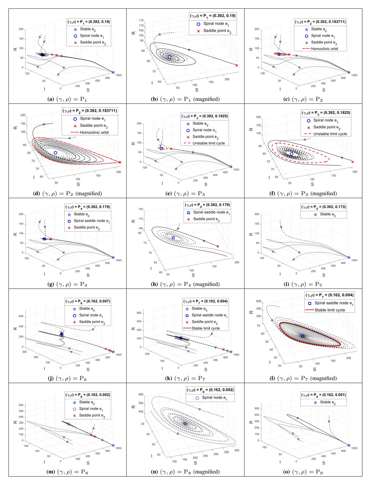
Figure 3: Phase portraits of the model (1) for (γ, ρ) = Pi, where i ∈ {1, . . . , 9}.
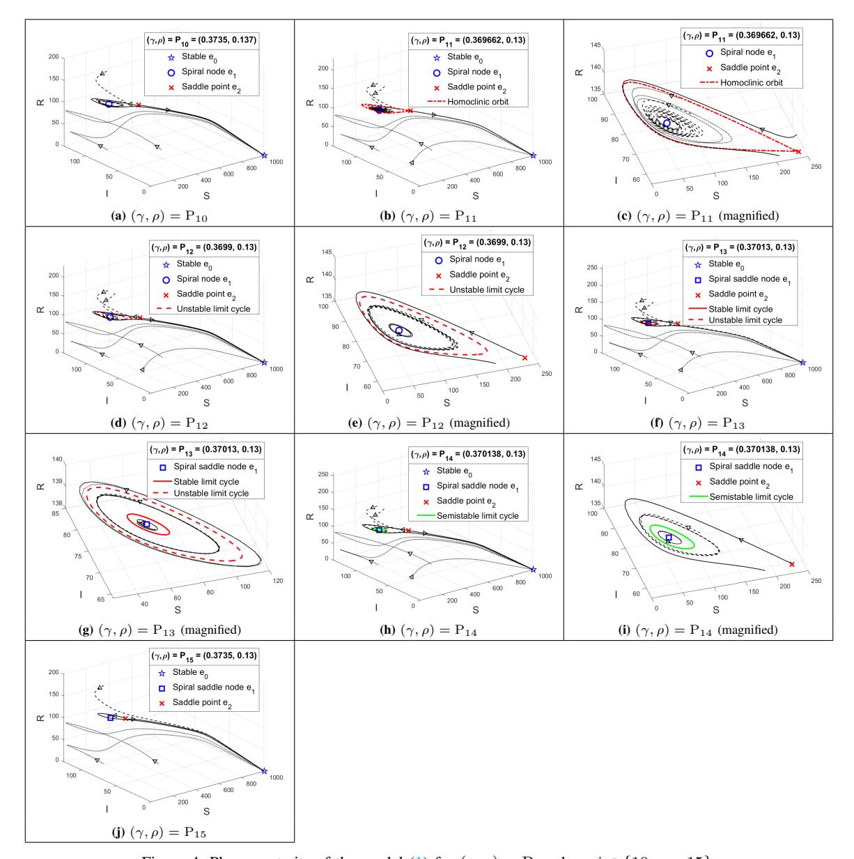
Figure 4: Phase portraits of the model (1) for (γ, ρ) = Pi, where i ∈ {10, . . . , 15}.
- (1) At ρ = 0.19, we have that (γ, ρ) = P1. Here, the stable disease-free equilibrium e0 coexist with two endemic equilibria: a stable spiral node e1 and a saddle point e2. Therefore, orbits may approach not only the disease-free equilibrium e0, but also the endemic equilibrium e1 (Figure 3 (a) and (b)). This means that, at this relatively high value of the hospitals' bed-occupancy rate, the disease may persist despite R0 < 1.
- (2) At ρ ≈ 0.183711, we have that (γ, ρ) = P2. At this point, the model undergoes a homoclinic bifurcation. The orbital behaviours remain qualitatively the same, except that a homoclinic orbit now emerges around the saddle endemic equilibrium e2, acting as a separatrix: orbits inside it approach e1, others approach e0 (Figure 3 (c) and (d)).
(3) At ρ = 0.1825, we have that (γ, ρ) = P3. Here, the homoclinic orbit has shrunk and become an unstable limit cycle, while remaining a separatrix in the sense previously described (Figure 3 (e) and (f)).
Both at ρ ≈ 0.183711 and at ρ = 0.1825, therefore, the possibility of the disease persisting even though R0 < 1 remains present. As we further decrease ρ, we arrive at ρ = ρA ≈ 0.181354, where the stable endemic equilibrium e1 absorbs the unstable limit cycle while losing its stability, via a subcritical Hopf bifurcation. This leaves no stable endemic equilibrium, and hence the disease's disappearance.
(4) At ρ = 0.179, we have that (γ, ρ) = P4. Here, no limit cycle exists, and the endemic equilibrium e1 has become a spiral saddle node. Since no endemic equilibria is stable, orbits approach the disease-free equilibrium e0 (Figure 3 (g) and (h)), meaning that the disease dies out.
Decreasing ρ further, one reaches the backward bifurcation threshold ρ = ρB ≈ 0.176117, where the two endemic equilibria e1 and e2 coalesce and disappear via a saddle-node bifurcation, leaving only the stable disease-free equilibrium e0.
(5) At ρ = 0.173, we have that (γ, ρ) = P5. Here, no endemic equilibria exist, and orbits still approach the stable disease-free equilibrium e0 (Figure 3 (i)).
From the perspective of the disease's eradication, this analysis highlights the importance of a low bedoccupancy rate. Specifically, for γ = 0.392, in order to guarantee the disease's disappearance, it is necessary to suppress the bed-occupancy rate to below the Hopf bifurcation point ρA. Notice, however, that ρA is larger than the backward bifurcation threshold, i.e., the saddle-node bifurcation point ρB.
3.2. The dynamical behaviour near BT2 and GH2
A magnification of Figure 3 near the Bogdanov-Takens bifurcation point BT2 is presented in Figure 2 (b). Comparing this to Figure 2 (a), one sees that around BT2, the model's orbital behaviours are qualitatively the same as those around BT1. Let us now turn our attention to the generalised Hopf bifurcation point GH2, near which a magnification of Figure 3 is displayed in Figure 2 (c). Here let us set γ = 0.162, and again observe the topological changes occurring as ρ is decreased gradually.
(6) At ρ = 0.007, we have that (γ, ρ) = P6. Here, no limit cycles exist, while two endemic equilibria coexist: the stable spiral node e1 and the unstable saddle point e2. Orbits are attracted by both e1 and the disease-free equilibrium e0 (Figure 3 (j)). Thus, as at P1, here we have the possibility of the disease continuing to exist despite R0 < 1.
As ρ is decreased from 0.007 to 0.004, it passes through a supercritical Hopf point ρ = ρC ≈ 0.002408, at which e1 loses stability while ejecting a stable limit cycle.
- (7) At ρ = 0.004, we have that (γ, ρ) = P7. Here, the presence of the stable limit cycle around e1 implies that the disease could still persist —with the number of infected individuals oscillating over time even though the endemic equilibria e1 and e2 are both unstable (Figure 3 (k) and (l)).
- (8) At ρ = 0.002, we have that (γ, ρ) = P8, and we have qualitatively the same behaviours as those at (γ, ρ) = P6 (Figure 3 (m) and (n)).
Finally, decreasing ρ further, we arrive at ρ = ρD ≈ 0.001573, where the two endemic equilibria coalesce and disappear in a saddle-node bifurcation.
(9) At ρ = 0.001, we have that (γ, ρ) = P9. Here, the only existing equilibria is the stable disease-free equilibrium e0 (Figure 3 (o)).
In the case of subsection 3.1, a complete eradication can already be guaranteed as soon as the bed-occupancy rate becomes lower than the Hopf bifurcation point ρA. In the present case, by contrast, it is necessary for to suppress the bed-occupancy rate to not merely below the Hopf bifurcation point ρC , but below the saddlenode bifurcation point, i.e., the backward bifurcation threshold ρD. Nevertheless, epidemiologically speaking, our conclusion from this analysis is similar, i.e., that a low bed-occupancy rate is necessary for a complete eradication. As strategies to suppress ρ, we recommend:
- reducing the number of patients having only mild symptoms by optimising self-isolation;
- transferring near-recovery patients from hospitals to hotels and apartments, so that more beds may be allocated to new patients and queues may be avoided;
- increasing hospital bed conversions for COVID-19 patients.
By keeping the susceptible individuals' cautiousness level γ constant, we have demonstrated the importance of having a low bed-occupancy rate ρ for the disease's eradication. In the next subsection, where we describe the orbital behaviours near GH1, we shall, in turn, fix a specific value of bed-occupancy rate ρ and see the importance of having a high susceptible individuals' cautiousness level γ.
3.3. The dynamical behaviour near GH1
We now consider the generalised Hopf bifurcation point GH1, in a neighbourhood of which the bifurcation diagram in Figure 1 is displayed in Figure 2 (d), with the addition of a homoclinic bifurcation curve, again plotted in red, and a saddle-node bifurcation of limit cycles curve, plotted in green.
(10) At (γ, ρ) = P10 = (0.3735, 0.137), the orbital behaviours are qualitatively the same as those at (γ, ρ) = P1 (Figure 4 (a)): no cycles exist, and orbits approach either e1 or e0.
Let us now fix ρ = 0.13, and describe the topological changes occurring as γ is increased gradually.
(11) At γ = γA ≈ 0.369662, we have that (γ, ρ) = P11, and that the model undergoes a homoclinic bifurcation: a homoclinic orbit emerges around the saddle endemic equilibrium e2, being a separatrix: orbits inside it approach the stable endemic equilibrium e1, others approach the disease-free equilibrium e0, as at (γ, ρ) = P2 (Figure 4 (b) and (c)). At this low cautiousness level, therefore, we still have the possibility of the disease persisting even though R0 < 1.
Increasing γ, the homoclinic orbit shrinks and becomes an unstable limit cycle, without abandoning its role as a separatrix.
(12) At γ = 0.3699, we have that (γ, ρ) = P12, and that the orbital behaviours are as at (γ, ρ) = P3 (Figure 4 (d) and (e)).
As γ is increased from 0.3699 to 0.37013, it passes through a subcritical Hopf bifurcation point γ = γB ≈ 0.370127, where stable endemic equilibrium e1 loses stability and ejects a stable limit cycle. Here we again have a situation where, although no stable endemic equilibrium exist, the disease could still persist due to the presence of a stable limit cycle.
- (13) At γ = 0.37013, we have that (γ, ρ) = P13, and that two limit cycles coexist, with opposite stabilities. Orbits near e1 approach the stable limit cycle, as also those in between the two limit cycles, while orbits outside the unstable limit cycle approach the disease-free equilibrium e0 (Figure 4 (f) and (g)).
- (14) At γ = γC ≈ 0.370138, we have that (γ, ρ) = P14, and that the two limit cycles coalesce in a saddle-node bifurcation of limit cycles, resulting in a single semistable limit cycle, orbits inside of which approach the limit cycle, while others approach e0 (Figure 4 (h) and (i)).
- (15) At γ = 0.3735, we have that (γ, ρ) = P15, and that the semistable limit cycle no longer exists, so that at (γ, ρ) = P15, orbits are attracted only by the disease-free equilibrium e0 (Figure 4 (j)). It is only at this stage that we are able to guarantee the disease's complete disappearance.
Therefore, for ρ = 0.13, we have seen that the disease's eradication can only be guaranteed when γ exceeds the backward bifurcation threshold γC . As strategies to increase γ, we recommend:
- optimising the use of media as tools to educate the public on the risks from COVID-19 and the efforts for prevention;
- continuing the campaign and enforcement of strict health protocols, so as to help breaking transmission chains.
4. CONCLUSIONS AND FUTURE RESEARCH
We have studied a mathematical model for the spread of COVID-19, which incorporates as two main parameters the susceptible individuals' cautiousness level γ and the hospitals' bed-occupancy rate ρ. A rectangular region exists on the γρ-plane where R0 < 1, the transcritical bifurcation at R0 = 1 is backward, and four codimension-two bifurcation points exist: two Bogdanov-Takens bifurcation points and two generalised Hopf bifurcation points. Our analysis near each bifurcation point has revealed the complex phenomena through which the model's asymptotic behaviour shifts from endemic to disease-free, which involves the births and disappearances of stable and unstable limit cycles and homoclinic orbits. From an epidemiological viewpoint, the analysis confirms the significance of the two parameters for the eradication of COVID-19. Indeed, the latter can be achieved, provided that susceptible individuals are sufficiently cautious of the disease's spread and thus implement the appropriate health protocols— and that serious efforts are made to keep the hospitals' bed-occupancy rate at a manageable level.
The codimension-two bifurcations described in this paper were discovered by choosing γ and ρ as bifurcation parameters. A similar investigation can be conducted by choosing as bifurcation parameters any other pair of parameters, to see whether codimension-two bifurcations also occur. Furthermore, as already noted in [27], the model studied in the present paper is much simplified, and so is modifiable in a number of ways, such as by introducing more compartments and the possibility of reinfection, as realised in [29]. In addition, since it is quite natural to suspect the nonlinear incidence rate βSI/(1 + γS) to be a main reason for the emergence of the complex behaviour studied in this paper, one could try replacing it with alternative forms of nonlinear incidence rate [13], [17], [26], such as
\[\frac{\beta SI}{1+\gamma S^p}\], \(\frac{\beta SI}{1+\gamma I^q}\), \(\frac{\beta SI}{1+\gamma_1 S^p+\gamma_2 I^q}\), \(\beta S^p I^q\), and investigate how the dynamical behaviour of the resulting model compares to that of the present model.
ACKNOWLEDGEMENT
This research was supported by Parahyangan Catholic University via the Dosen Muda research grant scheme 2022 (Number: III/LPPM/2022-02/23-P).