

1. INTRODUCTION
A plant is considered susceptible to infection when environmental factors alter its physiological processes, resulting in disruption of structure, growth, function, or other parameters. Plant diseases are classified into infectious and non-infectious according to the type of pathogen. Symptoms of the disease depend on its cause, nature and location of the affected area. Plant disease-causing factors can be both biotic and abiotic in nature. Non-infectious diseases are caused by unfavourable growing conditions. They are not transferred from diseased plants to healthy plants. On the other hand, infectious diseases can multiply inside or on the surface of plants, so infections can spread from one susceptible host to another [31].
Various infectious diseases that are frequently brought on by fungi, viruses, or bacteria affect plant ecological populations. These diseases can range in severity from minor leaf or fruit damage to death, and as a result, the plant populations lose their fertility, which causes a reduction in their population size. Some of the most prominent plant diseases are Algal leaf spot of tea: (Cephaleuros virescens), Pineapple mealybug: (Dysmicoccus brevipes), Brown Spot: (Helminthosporium oryzae), Cedar Apple Rust (Gymnosporangium juniperi-virginianae Schwein), Red rot: (Glomerella tucumanensis) and so on. Crop damage due to pests is a major cause of concern worldwide. According to a recent report released by the U.N. Food and Agriculture Organization in 2021, about 40 percent of the world's agricultural crops are lost to pests each year. Therefore, it is important to study plant infectious diseases in the ecosystem and find ways to control these diseases. One of the significant ways of combatting pests is the utilisation of pesticides which in the 21st century has become more and more necessary. In India, the production of pesticides began in 1952 with the construction of the BHC manufacturing plant near Calcutta, and India is presently the second largest producer of pesticides
*Corresponding author in Asia after China and is ranked 12th in the world (Mathur, 1999) [29]. Pesticides are compounds that are intended to control various pests and disease carriers such as mosquitoes, ticks, mice and rodents. Although the use of pesticides has both a positive and negative impact, one cannot deny the significance it has in the agricultural sector [24]. In recent times, the use of pesticides has become significantly important in farming as it helps farmers in controlling weeds, insect invasion and any other diseases that can cause damage to the crops.
"Mathematical Biology" [11], [2], [21] is a rapidly evolving, well-defined field of study and the most exciting application of mathematics today. Biology as a science helps human health in many ways, so expanding the scope of biomathematics is inevitable. It helps to increase food production, fight disease and also helps to protect and preserve our environment. Mathematical modelling has been used extensively in successfully defining the Biological system. It also provides guidelines for scientists, physicians or policymakers to make informed decisions. There are a number of problems in the biological system, especially in ecosystems and epidemics, that still need to be identified where mathematical modelling can make a difference. Eykhoff (1974) defines a mathematical model as a "representation of the essential elements of an existing system (or system to be constructed) that present the information of that system in a practical way". An ecosystem is a system of a community or group of living organisms that live and communicate with each other in a given environment at a specific time. An ecosystem consists of biotic (living) and abiotic (non-living) and is of different types such as Plant Ecosystem, Forest Ecosystem, Desert Ecosystem, Grassland Ecosystem, Mountain Ecosystem, Marine Ecosystem, Freshwater Ecosystem and so on. An Epidemic describes diseases that may occur in that ecosystem at a given time. Hence an Eco-epidemic model is a mathematical representation that describes the ecosystems of interacting populations when there is the presence of disease in that population [3], [4], [8], [14], [15].
According to Indiati et al. [16], one way to control pests in plants is by spraying pesticides with the right amount of dose. The inappropriate use of pesticides may have a serious negative impact on the environment and can be hazardous to human health [16]. In India, an excessive amount of pesticide is used during cultivation whereby some part of it is mixed with surface and underground runoff, eventually reaching the water bodies, and the soil absorbs the other part, and hence this pollutes both soil and groundwater [24]. Considering this scenario, Kumar et al. [24] studied the harmful effect of pesticides on groundwater contamination during cultivation. As pest control is now a global problem due to population growth, appropriate techniques are needed to control pest populations, and farmers' agricultural awareness is equally important in pest control [18]. Effective pest control strategies, therefore, have a significant impact on society. Hence, effective use of predators and appropriate use of chemicals or pesticides are highly recommended to control pest populations [18]. Irham et al. [17] developed a mathematical model to observe the interactions between two predators and infected prey, and the prey is controlled by the use of pesticides. They considered a functional response Holling type II, where they found out that upon utilisation of pesticides, if the pest growth is lower than the death rate, then all predators and prey will become extinct and be locally asymptotically stable. On the other hand, if the pest growth is higher than the death rate, then only vulnerable pests remain alive, while other pests will die and are asymptotically stable. All of these populations affected by pesticide control and predation rates can survive.
In recent years, various research has been conducted in the study of infectious disease in plant populations through the use of control measures such as pesticides and natural predators with the aim of controlling crop damage against pests [36], [37], [9], [5]. In this study, we have paid attention to the utilisation of pesticides and the harmful effects of pests on plants. Harmful insect pests consist of caterpillars, grasshoppers and locusts, which devour the leaves, seeds and culmination of crops. At times, locusts can shape a large plague of several million that could cause big damage to plants and cause famine. Other insects, together with aphids, thrips and weevils, suck the sap from plants, which can affect plant boom and improvement and make plants greater susceptible to disease. During the literature survey, it was observed that negligible importance is given to plant population models with the application of pesticides. The existence of plant infections often results in the necessity of applying pesticides. However, the decision to use pesticides relies on various biotic factors and the farmer's overall management practices. Farmers may opt for pesticide usage to control pathogen spread in certain cases. Sometimes contagious pathogen-based diseases can only be eradicated using pesticides, e.g., Colorado potato beetle (Leptinotarsa decemlineata). This beetle is a common and highly destructive pest that feeds on potato plants and can cause significant damage to the crop. Pesticides specifically formulated to target Colorado potato beetles, such as insecticides containing active ingredients like imidacloprid or spinosad, can be applied to control their population and prevent widespread infestation [20]. In such a scenario, farmers are indirectly forced to use pesticides to control the disease. Assuming this indirect effect, we introduced a new factor, namely infective induced rate of pesticides which work as a source in the pesticide compartment. Our work contributes to the field by introducing this new term and offers new avenues for future research in SIR modelling.
The structure of the paper is as follows: Section 2 addresses the formulation of a mathematical model and associated assumptions. In section 3, the theoretical analysis of the proposed model is presented. The positivity and boundedness of the model, along with the uniqueness and existence of solutions, have been discussed therein. The conditions for the existence of all possible equilibrium points, along with the basic reproduction number and the stability analysis, have thoroughly been studied. With the help of sensitivity index analysis, the rate of change of the basic reproduction number towards its parameters and Hopf bifurcation of the system have also been discussed in section 3. In section 4, numerical simulations that clarify the analysis results obtained are discussed along with comparisons of susceptible, infected, recovered, and pesticides vs time with control. Finally, brief conclusions and discussions were given in section 5. Analytical computations and numerical simulations were carried out with the help of advanced software like Mathematica, Matlab, and MatCont 7.3.
2. MODEL FORMULATION
To form the mathematical model, the following assumptions are taken into consideration:
- 1) In the absence of disease, the plant population grows logistically with an intrinsic growth rate r > 0 and environmental carrying capacity k > 0.
- 2) In the presence of the disease, the plant population is divided into three compartments: the susceptible population S(t), the infected population I(t) and the recovered population R(t). Therefore, for any time t, the total plant population is given by S(t) + I(t) + R(t) = N(t). Then the growth rate of the susceptible plant population is given by \(rS\left(1 \frac{N}{k}\right)\) or \(rS\left(1 \frac{S + I + R}{k}\right)\).
- The susceptible population becomes infected when they come into contact with infected populations. This contact process is assumed to follow the kinetics of simple mass action using \(\beta > 0\) as the conversion factor.
- 4) Only the susceptible population S(t) can reproduce and the death rate of plants due to pests is assumed to be \(\mu > 0\). The natural mortality rate of plants is ignored from the incubation period to the death of the plants. However, the infected population I contributes with S to population growth towards the carrying capacity k > 0.
- 5) As a control measure, we assume that a general pesticide P(t) is used to minimize diseases in the population. Due to the application of pesticides, plants within the infected compartment transition to the recovered compartment and eventually return to a susceptible compartment within a specific timeframe. Pesticides are used in both susceptible and infected populations, and it is assumed that the use of pesticides has negative impacts on both the susceptible and the infected populations. The negative impact of pesticides is ignored for the plant population in the recovered compartment, as they have already been exposed to the pathogen or pest and have developed immunity or resistance against it. Also, the recovered population eventually reverts to a susceptible state after a certain time. For instance, Propiconazole and Tricyclazole are two common fungicides primarily targeted at controlling fungal diseases like blast disease and dirty panicle disease in rice crops. They are not intended to harm non-infected rice plants [22]. Still, their residues and potential for phytotoxicity emphasize the importance of responsible and precise application, that can range from mild stress symptoms to severe damage and plant death.
- 6) The amount of pesticides used is just one of several factors that can influence the contact rate between plants populations and pesticides. Let the amount of pesticide used to be \(\alpha>0\). The contact rate between susceptible plants and pesticides is assumed to be \(\tilde{d}_1(\alpha)>0\). Similarly, the contact rate between infected plants and pesticides is assumed to be \(\tilde{d}_2(\alpha)>0\). Here we consider \(\tilde{d}_i(\alpha)=d_i, i=1,2\), where \(d_i\) are constants. Therefore, the term \(-d_1SP\) represents the removal of plants from susceptible plant compartment due to the application of pesticides. The term \(-d_2IP\) represents the removal of plants from infected plant compartment due to the application of pesticides.
- 7) The presence of plant infections can often lead to the application of pesticides. However, the decision to use pesticides depends on various factors, including the severity of the infection, the type of pathogen
involved, the crop being grown, and the overall management practices employed by the farmer. When plants are infected by pathogens, it can lead to the development of plant diseases, which can impact the health and productivity of the crop. In some cases, farmers may choose to use pesticides to control the spread of the pathogens and mitigate the damage caused by the disease. Pesticides specifically formulated to target the pathogens causing the infection may be employed as a means to suppress or eliminate them. Therefore we assumed that the infections in plants indirectly forces the farmers to apply pesticides. The term \(\theta I\), \(\theta > 0\) denotes the infective induced rate of pesticides.
- 8) The application of pesticides enhances the recovery rate of the infected plants. Let g > 0 be the recovery rate of the infected plants due to the application of pesticides.
- 9) Let \(\nu > 0\) be the rate of infected plants which have recovered and returned to the susceptible class [27], [1].
| Variables | Definitions | Units |
|---|---|---|
| S(t) | Susceptible population | [Stems] |
| I(t) | Infected population | [Stems] |
[SI unit]
[Stems]
Pesticides
P(t)
R(t)
Table 1: Notations and definition of model variables.
Table 2: Notations and definition of model parameters
Recovered population
| Parameters | Definitions | Units |
|---|---|---|
| r | Intrinsic growth rate of the plant population | Per day |
| k | Environmental carrying capacity | Per sq. meter |
| \(\beta\) | Contact rate between susceptible and infected plants | Per day |
| \(d_1\) | Contact rate between susceptible and pesticides | Per day |
| \(d_2\) | Contact rate between infected plants and pesticides | Per day |
| \(\mu\) | Death rate of plants due to pests | Per day |
| \(\nu\) | Rate of infected plants which have recovered and returned to the susceptible class | Per day |
| g | Recovery rate of infected plants | Per day |
| \(\overset{\circ}{\theta}\) | Infective induce rate of pesticides | Per day |
| \(\alpha\) | Amount of pesticides used | Per day |
In accordance with the above assumptions and the descriptions of variables and parameters, the present model will be governed by the following system of equations:
\[\frac{dS}{dt} = rS\left(1 - \frac{S + I + R}{k}\right) - \beta SI - d_1 SP - \mu S + \nu R,\] \[\frac{dI}{dt} = \beta SI - (g + \mu)I - d_2 IP,\] \[\frac{dP}{dt} = \theta I - \alpha P,\] \[\frac{dR}{dt} = gI - (\mu + \nu)R,\] (1)
with initial conditions:
\[S(0) = S_0 > 0, I(0) = I_0 > 0, P(0) = P_0 > 0 \text{ and } R(0) = R_0 > 0.\] (2)
Here \(\frac{dS}{dt}, \frac{dI}{dt}, \frac{dP}{dt}\) and \(\frac{dR}{dt}\) represents the rates of change of the quantities S(t), I(t), P(t) and R(t) respectively.
3. MODEL ANALYSIS
3.1. Positivity and Boundedness
Theorem 3.1. (Positivity): All solutions of the system represented by (1) with initial conditions (2) are positive for all \(t \ge 0\).
Proof: Let S(t), I(t), P(t), R(t) be the solutions of System (1) with initial conditions (2). Integrating both sides of the first equation of (1) from 0 to t, gives,
\[\frac{dS}{dt} = rS\left(1 - \frac{S + I + R}{k}\right) - \beta SI - d_1SP - \mu S + \nu R \ge -\left\{\beta SI + d_1SP + \mu S - rS\left(1 - \frac{S + I + R}{k}\right)\right\},\]
oı
\[\int_0^t \frac{dS}{S} \ge \int_0^t -\left\{\beta I + d_1 P + \mu - r\left(1 - \frac{S + I + R}{k}\right)\right\} dt,\] or
\[S(t) \ge S(0) \exp\bigg[\int_0^t -\left\{\beta I + d_1 P + \mu - r\left(1 - \frac{S + I + R}{k}\right)\right\} dt\bigg],\] \[\implies S(t) > 0.\]
From the second equation of System (1), we get
\[I(t) \ge I(0) \exp\left[\int_0^t \left\{\beta SI - (g+\mu)I - d_2 IP\right\} dt\right],\]
\[\Rightarrow I(t) > 0.\]
From the third equation of System (1), we get
\[P(t) \ge P(0) \exp\bigg[\int_0^t -\alpha P dt\bigg],\] \[\implies P(t) > 0.\]
From the fourth equation of System (1), we get
\[R(t) \ge R(0) \exp\left[\int_0^t \left\{-(\mu + \nu)R\right\} dt\right],\] \[\implies R(t) > 0.\]
Hence, the theorem is proved.
Theorem 3.2. (Boundedness): All solutions of System (1) that start in \(R^4_+\) are uniformly bounded in the solution set \(\Omega = \left\{ (S, I, P, R) : 0 \le S \le \frac{rk}{4\mu}, 0 \le I \le \frac{rk}{4\mu}, 0 \le R \le \frac{rk}{4\mu}, 0 \le P \le \frac{rk\theta}{4\alpha\mu}, 0 \le S + I + R \le \frac{rk}{4\mu} \right\}.\)
Proof: Let S(t), I(t), P(t), R(t) be the solution of System (1). Let W=S+I+R
\[\begin{split} \frac{dW}{dt} &= \frac{dS}{dt} + \frac{dI}{dt} + \frac{dR}{dt} \\ &= rS\left(1 - \frac{S}{k}\right) - \mu(S + I + R) - d_1SP - d_2IP - rS\left(\frac{I + R}{k}\right), \\ \Longrightarrow \frac{dW}{dt} + \mu W \leq rS\left(1 - \frac{S}{k}\right). \end{split}\]
\[\begin{array}{l} \text{Let } f(S) = rS\left(1-\frac{S}{k}\right). \\ \text{Therefore, } \frac{df}{dS} = r - \frac{2rS}{k} \text{ and } \frac{d^2f}{dS^2} = -\frac{2r}{k}. \\ \text{Now, } \frac{df}{dS} = 0 \implies r - \frac{2rS}{k} = 0 \implies S = \frac{k}{2} \end{array}\]
Then \(\frac{d^2f}{dS^2} = -\frac{2r}{k} < 0\), which gives a maximum value for S.
Therefore \(\frac{dW}{dt} + \mu W \leq \frac{rk}{4} \implies W \leq \frac{rk}{4\mu} + \left(W_0 - \frac{rk}{4\mu}\right)e^{-\mu t}\). As \(t \to \infty\), \(e^{-\mu t} \to 0 \implies W \to \frac{rk}{4\mu} \implies W(t) \leq \frac{rk}{4\mu}\) and hence W is bounded. Clearly I(t) is bounded above by \(\frac{rk}{4\mu}\). Therefore, the third equation of System (1) becomes
\[\frac{dP}{dt} + \alpha P \le \frac{rk\theta}{4\mu},\] \[\implies P \le \frac{rk\theta}{4\alpha\mu} + \left(P_0 - \frac{rk\theta}{4\alpha\mu}\right)e^{-\alpha t},\]
where \(P_0\) is the initial amount of pesticide used. As \(t \to \infty\), \(e^{-\alpha t} \to 0 \implies P \to \frac{rk\theta}{4\alpha\mu} \implies P(t) \le \frac{rk\theta}{4\alpha\mu}\) and hence P is bounded for any initial value and for all t. Therefore S(t), I(t), P(t), R(t) are uniformly bounded.
Note: From Theorem 3.2, it is clear that each population is bounded above. So the total population N(t) is also bounded above whenever time \(t \to \infty\).
3.2. Existence and Uniqueness of Solution for the SIPR Model
In this section, we formulate the existence and uniqueness theorem of System (1). Following the method used by Samuel et al. [33], we perform the proof of the following theorems. The general first-order ODE is in the form:
\[x' = f(t, x), x(t_0) = x_0. (3)\]
One could be interested in asking the following questions:
- 1) Under what conditions the solution of Equation (3) exists?
- 2) Under what conditions Equation (3) has a unique solution?
To answer the above question, we use the following theorem
Theorem 3.3. (Uniqueness of Solution): Let D denote the region:
\[|t - t_0| \le a, ||x - x_0|| \le b, x = (x_1, x_2, x_3, \dots, x_n), x_0 = (x_{10}, x_{20}, x_{30}, \dots, x_{n0}).\] \[(4)\]
Suppose the function f(t,x) satisfies the Lipschitz condition:
\[||f(t,x_1) - f(t,x_2)|| \le M||x_1 - x_2||, \tag{5}\]
and whenever \((t, x_1)\) and \((t, x_2)\) belong to the region D and M represent a positive constant. Then, \(\exists\) a constant \(\delta > 0\) such that there exists a unique continuous vector solution x(t) of the system 3 in the interval \(|t-t_0|<\delta\).
Remark 1. It is important to note that condition (5) is satisfied by the requirement that:
\[\frac{\partial f_i}{\partial x_j}\], \(i, j = 1, 2, \dots n\), is continuous and bounded in the region D.
Lemma 3.4. If f(t,x) has continuous partial derivative \(\frac{\partial f_i}{\partial x_i}\) on a bounded closed convex domain \(\mathcal{R}\) (i.e., convex set of real numbers), where R is used to denotes real numbers, then it satisfies a Lipschitz condition in R.
Our interest is in the domain
\[1 \le \epsilon \le \mathcal{R}. \tag{6}\]
So, we look for a bounded solution of the form \(0 < \mathcal{R} < \infty\). We now prove the following existence theorem.
Theorem 3.5. (Existence of solution): Let D denote the region defined in (4) such that (5) and (6) holds. Then, there exists a solution of the equations of System (1) which is bounded in the region D.
Proof: From System (1), Let,
\[f_1 = rS\left(1 - \frac{S + I + R}{k}\right) - \beta SI - d_1 SP - \mu S + \nu R,\tag{7}\]
\[f_2 = \beta SI - (g + \mu)I - d_2 IP, \tag{8}\]
\[f_3 = \theta I - \alpha P,\tag{9}\]
\[f_4 = gI - (\mu + \nu)R. \tag{10}\]
We show that \(\frac{\partial f_i}{\partial x_j}\), \(i, j = 1, 2, \dots, n\) are continuous and bounded. We consider the following partial derivatives for all the model equations:
From Equation (7):
\[\left| \frac{\partial f_1}{\partial S} \right| = \left| r \left( 1 - \frac{2S + I + R}{k} \right) - \beta I - d_1 P - \mu \right| < \infty, \left| \frac{\partial f_1}{\partial I} \right| = \left| \frac{-(r + \beta k)S}{k} \right| < \infty,\] \[\left| \frac{\partial f_1}{\partial P} \right| = \left| -d_1 S \right| < \infty, \quad \left| \frac{\partial f_1}{\partial R} \right| = \left| \frac{-rS}{k} - \nu \right| < \infty.\]
From Equation (8):
\[\left| \frac{\partial f_2}{\partial S} \right| = |\beta I| < \infty, \quad \left| \frac{\partial f_2}{\partial I} \right| = |\beta S - (g + \mu) - d_2 P| < \infty,\] \[\left| \frac{\partial f_2}{\partial P} \right| = |-d_2 I| < \infty, \left| \frac{\partial f_2}{\partial R} \right| = 0 < \infty.\]
From Equation (9):
\[\left| \frac{\partial f_3}{\partial S} \right| = 0 < \infty, \left| \frac{\partial f_3}{\partial I} \right| = |\theta| < \infty,\] \[\left| \frac{\partial f_3}{\partial P} \right| = |-\alpha| < \infty, \left| \frac{\partial f_3}{\partial R} \right| = 0 < \infty.\]
From Equation (10):
\[\left| \frac{\partial f_4}{\partial S} \right| = 0 < \infty, \left| \frac{\partial f_4}{\partial I} \right| = |g| < \infty,\] \[\left| \frac{\partial f_4}{\partial P} \right| = 0 < \infty, \left| \frac{\partial f_4}{\partial R} \right| = |-(\mu + \nu)| < \infty.\]
We have clearly established that all these partial derivatives are continuous and bounded in D. Hence, by Theorem (3), there exists a unique solution of the system (1) in the region D.
Hence, the positivity (Theorem 3.1), boundedness (Theorem 3.2) and the uniqueness existence (Theorem 3.3) of System (1) implies that the model is biologically valid and well behaved.
3.3. Equilibrium points
For finding the equilibrium points, we set the right-hand side of System (1) equals to zero as follows:
\[\begin{split} \frac{dS}{dt} &= rS\left(1 - \frac{S + I + R}{k}\right) - \beta SI - d_1 SP - \mu S + \nu R = 0, \\ \frac{dI}{dt} &= \beta SI - (g + \mu)I - d_2 IP = 0, \\ \frac{dP}{dt} &= \theta I - \alpha P = 0, \\ \frac{dR}{dt} &= gI - (\mu + \nu)R = 0. \end{split}\]
On solving the above equations, then three equilibrium points in the coordinate \((S^*, I^*, P^*, R^*)\) are obtained and are given as follows:
- (i) The trivial equilibrium point \(T_0(0,0,0,0)\).
- Disease-free equilibrium point \(T_1\left(\frac{k(r-\mu)}{r},0,0,0\right)\). It is seen that the equilibrium point \(T_1\) consistently exists if and only if \(r > \mu\).
- The disease-endemic equilibrium point \(T_2(S^*, I^*, P^*, R^*)\) which is explicitly expressed in term of \(I^*\)
\[S^* = \frac{1}{\alpha\beta}[d_2\theta I^* + \alpha(g+\mu)], P^* = \frac{\theta}{\alpha}I^*, R^* = \frac{gI^*}{\mu+\nu}\] and \(I^*\) is a positive root of the following equation
\[\Psi_1(I^*)^2 + \Psi_2I^* + \Psi_3 = 0, \tag{11}\]
where,
\[\begin{split} &\Psi_1 = \frac{\alpha d_2 \theta(r+\beta) + k d_1 d_2 \theta^2}{\alpha^2 \beta} + r \left(\frac{d_2 \theta}{\alpha \beta}\right)^2 - \frac{\alpha \beta r g d_2 \theta}{\mu + \nu}, \\ &\Psi_2 = \frac{\alpha \beta [\alpha (\alpha + \beta) (g + \mu) + k \mu \theta + k d_1 \theta(g + \mu)] + \alpha \theta d_2 [(r+1) (g + \mu) - \beta r]}{(\alpha \beta)^2} + \frac{\alpha \beta g [\alpha \beta k \nu - \alpha r (g + \mu)]}{\mu + \nu}, \\ &\Psi_3 = \frac{(g + \mu) [k \mu + \alpha^2 \beta (g + \mu - \beta k)]}{\beta}. \end{split}\]
Equation (11) implies,
\[I^{*2} + M_1 I^* + M_2 = 0, (12)\]
where \(M_1=\Psi_2/\Psi_1,\ M_2=\Psi_3/\Psi_1.\) From Equation (12), \(I^*>0\) if one of the following conditions holds:
- (a) \(\dot{M}_1 < 0, \ M_2 < 0,\)(b) \(\dot{M}_1 < 0, \ \dot{M}_2 > 0\) and \(\dot{M}_1^2 4M_2 > 0,\)
- (c) \(M_1 > 0, M_2 < 0.\)
Real and positive solutions of \(I^*\) give \(S^* > 0, P^* > 0\). Due to the complexity of the model, it is hard to determine the analytical solutions. So we proceed our discussions using numerical techniques.
3.4. Basic Reproduction Number \(R_0\)
In this section, we determine the basic reproduction number \(R_0\). This can be characterised as the average number of secondary infections caused by typical cases of infection in the general population, which is vulnerable to everyone. \(R_0\) is basically used to measure the potential for transmission of a disease.
Theorem 3.6. The basic reproduction number of the system (1) is given by \(R_0 = \frac{\beta k(r-\mu)}{r(q+\mu)}\)
Proof: The Basic reproduction number \(R_0\) is calculated with the help of the next generation matrix method which is given by \(G = FV^{-1}\) [19], where F is the newly formed infection matrix, V is the transmitted infection matrix and \(V^{-1}\) is the inverse of V. So,
\[F_i = \left( \begin{array}{c} \beta SI \\ 0 \\ 0 \end{array} \right), \quad V_i = \left( \begin{array}{c} \left( d_2P + g + \mu \right)I \\ \alpha P - \theta I \\ R(\mu + \nu) - gI \end{array} \right), \quad \text{where} \ \ i = 1, 2, 3.\]
Therefore
\[F = \begin{pmatrix} \beta S & 0 & 0 \\ 0 & 0 & 0 \\ 0 & 0 & 0 \end{pmatrix}, \quad V = \begin{pmatrix} d_2 P + g + \mu & d_2 I & 0 \\ -\theta & \alpha & 0 \\ -g & 0 & \mu + \nu \end{pmatrix}.\]
At the disease-free equilibrium \(T_1\), we have
\[F = \begin{pmatrix} \frac{\beta k(r-\mu)}{r} & 0 & 0 \\ 0 & 0 & 0 \\ 0 & 0 & 0 \end{pmatrix}, \text{ and } V = \begin{pmatrix} g+\mu & 0 & 0 \\ -\theta & \alpha & 0 \\ -g & 0 & \mu+\nu \end{pmatrix} \implies V^{-1} = \begin{pmatrix} \frac{1}{g+\mu} & 0 & 0 \\ \frac{\theta}{\alpha(g+\mu)} & \frac{1}{\alpha} & 0 \\ \frac{-g}{(g+\mu)(\mu+\nu)} & 0 & \frac{1}{\mu+\nu} \end{pmatrix}.\]
Therefore \(G=FV^{-1}=\left( \begin{array}{ccc} \frac{\beta k(r-\mu)}{r(g+\mu)} & 0 & 0 \\ 0 & 0 & 0 \\ 0 & 0 & 0 \end{array} \right)\) and the basic reproduction number is the dominant eigenvalue of G which is given by:
\[R_0 = \frac{\beta k(r-\mu)}{r(g+\mu)}. (13)\]
Remark 2. The local dynamics of the SIPR model is analysed by the reproduction number \(R_0\). From the dynamics of the system, if \(R_0 < 1\), the number of infections in the plants population will decrease and eventually the disease will disappear. If \(R_0 > 1\), the disease is more likely to be transmitted between different plants in the population and there will be a possibility of an outbreak of the disease. \(R_0 = 1\) acts as a disease threshold, that is, the disease remain active and stable, but the chances of an outbreak or epidemic of the disease are very limited [7].
3.5. Stability Analysis
In order to study the stability properties, the general Jacobian matrix J of the system (1) is reported as follows:
\[J = \begin{pmatrix} J_{11} & \frac{-(r+\beta k)S}{k} & -d_1 S & \frac{k\nu - rS}{k} \\ \beta I & J_{22} & -d_2 I & 0 \\ 0 & \theta & J_{33} & 0 \\ 0 & q & 0 & J_{44} \end{pmatrix},\](14)
where,
\[\begin{split} J_{11} &= r \left( 1 - \frac{2S + I + R}{k} \right) - \beta I - d_1 P - \mu, \\ J_{22} &= \beta S - (g + \mu) - d_2 P, \\ J_{33} &= -\alpha, \\ J_{44} &= -(\mu + \nu). \end{split}\]
1) Stability of trivial equilibrium point:
Theorem 3.7. The trivial equilibrium point \(T_0(0,0,0,0)\) is stable if \(r < \mu\) and unstable if \(r > \mu\).
Proof: The Jacobian matrix of System (1) at \(T_0\) is given by
\[J_{T_0} = \begin{pmatrix} r - \mu & 0 & 0 & \nu \\ 0 & -(g + \mu) & 0 & 0 \\ 0 & \theta & -\alpha & 0 \\ 0 & g & 0 & -(\mu + \nu) \end{pmatrix}.\]
The eigenvalues of the above matrix are:
\[\lambda_1 = r - \mu\], \(\lambda_2 = -(g + \mu)\), \(\lambda_3 = -\alpha\) and \(\lambda_4 = -(\mu + \nu)\).
Clearly, \(\lambda_2, \lambda_3, \lambda_4 < 0\). If \(r - \mu < 0\), then \(\lambda_1 < 0\) and the equilibrium \(T_0\) is stable and unstable otherwise. Hence, \(T_0\) is stable if \(r < \mu\) and unstable if \(r > \mu\).
2) Local stability of the disease-free equilibrium:
Theorem 3.8. The disease-free equilibrium \(T_1\left(\frac{k(r-\mu)}{r},0,0,0\right)\) is locally asymptotically stable if \(R_0<1\) and unstable if \(R_0>1\).
Proof: The Jacobian matrix of System (1) at \(T_1\) is given by:
\[J_{T_1} = \begin{pmatrix} -(r-\mu) & \frac{-(r+\beta k)(r-\mu)}{r} & \frac{-d_1 k(r-\mu)}{r} & \nu - (r-\mu) \\ 0 & \frac{\beta k(r-\mu)}{r} - (g+\mu) & 0 & 0 \\ 0 & \theta & -\alpha & 0 \\ 0 & g & 0 & -(\mu+\nu) \end{pmatrix}.\](15)
Eigenvalues of the above matrix (15) are:
\[\lambda_1 = -(r - \mu), \ \lambda_2 = \frac{\beta k(r - \mu)}{r} - (g + \mu), \ \lambda_3 = -\alpha \text{ and } \lambda_4 = -(\mu + \nu).\]
Clearly, \(\lambda_1, \lambda_3, \lambda_4 < 0\).
Now, for System (1) to be stable at \(T_1\), we must have \(\lambda_2 < 0\), i.e.,
\[\frac{\beta k(r-\mu)}{r} - (g+\mu) < 0\] \[\implies \frac{\beta k(r-\mu)}{r} < (g+\mu)\] \[\implies \frac{\beta k(r-\mu)}{r(g+\mu)} < 1\] \[\implies R_0 < 1.\]
Thus, \(\lambda_2 < 0\) if \(R_0 < 1\), which implies all the eigenvalues of the characteristic equation (15) have a negative real parts. Hence the equilibrium \(T_1\) is locally asymptotically stable.
3) Local stability of the endemic equilibrium:
Theorem 3.9. The endemic equilibrium \(T_2(S^*, I^*, P^*, R^*)\) is locally asymptotically stable if the following condition holds [34]:
\[A_1 > 0\], \(A_3 > 0\), \(A_4 > 0\) and \(A_1 A_2 A_3 > A_3^2 + A_1^2 A_4\), where,
\[A_{3} = r \left( \frac{2S^{*} + I^{*} + R^{*}}{k} - 1 \right) - \beta(S^{*} - I^{*}) + (d_{1} + d_{2})P^{*} + (3\mu + g + \alpha + \nu),\] \[A_{2} = G_{1} + \alpha(\mu + \nu) - (\alpha + \nu + \mu)G_{2} + \frac{\beta(r + \beta k)S^{*}I^{*}}{k},\] \[A_{1} = \alpha(\mu + \nu)G_{3} + (\alpha + \mu + \nu) \left( G_{1} + \frac{\beta(r + \beta k)S^{*}I^{*}}{k} \right) + d_{1}\beta\theta S^{*}I^{*} - d_{2}\theta I^{*} - \frac{g\beta(k\nu - rS^{*})I^{*}}{k},\] \[A_{0} = \alpha(\mu + \nu) \left( G_{1} + \frac{\beta(r + \beta k)S^{*}I^{*}}{k} \right) - (\mu + \nu)(d_{2}\theta I^{*} - d_{1}\beta\theta S^{*}I^{*}) - \frac{\alpha\beta g(k\nu - rS^{*})I^{*}}{k}.\]
Here
\[G_1 = (\beta S^* - d_2 P^* - g - \mu) \left( r - \mu - \beta I^* - d_1 P^* - \frac{(2S^* + I^* + R^*)r}{k} \right),\] \[G_2 = \beta (S^* - I^*) + (r - g - 2\mu) - (d_1 + d_2) P^* - \frac{(2S^* + I^* + R^*)r}{k},\] \[G_3 = \frac{(2S^* + I^* + R^*)r}{k} + 2\mu + g + (d_1 + d_2) P^* - \beta (S^* - I^*) - r.\]
Proof: The characteristic roots corresponding to the equilibrium \(T_2\) are given by the equation:
\[\xi^4 + A_3 \xi^3 + A_2 \xi^2 + A_1 \xi + A_0 = 0. {16}\]
By Routh-Hurwitz criterion, the equation will have negative roots if
\[A_1 > 0, A_3 > 0, A_4 > 0\] and \(A_1 A_2 A_3 > A_3^2 + A_1^2 A_4\). (17)
Hence \(T_2\) is locally asymptotically stable if the above conditions are satisfied and unstable otherwise.
3.6. Sensitivity analysis of the basic reproduction number
The basic reproduction number \(R_0\) is a function of five parameters \(\beta, k, r, \mu, g\). To understand the contribution of each of the parameters in the Reproduction number \(R_0\) as given by (13), a sensitivity analysis [35] is being conducted which let us know how significant each parameter is to a disease transmission. Sensitivity index of the system is given as:
\[S_h^{R_0} = \frac{h}{R_0} \frac{\partial R_0}{\partial h}.\] (18)
The sensitivity indices of the reproduction number with respect to \(\beta\), k, r, \(\mu\), g are given by:
\[S_{\beta}^{R_0} = 1\], \(S_k^{R_0} = 1\), \(S_r^{R_0} = \frac{\mu}{r - \mu}\), \(S_{\mu}^{R_0} = \frac{-\mu(g + r)}{(r - \mu)(q + \mu)}\), \(S_g^{R_0} = \frac{-g}{q + \mu}\).
The index table is shown in Table 3:
Table 3: Sensitivity index table.
| Parameters | Sensitivity index | Sensitivity index values |
|---|---|---|
| \(\beta\) | 1 | 1/day |
| k | 1 | \(1/m^2\) |
| r | \(\frac{\mu}{r-\mu}\) | 0.029/day |
| \(\mu\) | \[\frac{\frac{r}{r-\mu}}{\frac{-\mu(g+r)}{(r-\mu)(g+\mu)}}\] \[\frac{\frac{-g}{g+\mu}}\] | -0.938/day |
| g | \(\frac{-g}{g+\mu}\) | -0.091/day |
From Table 3, it can be seen that the sensitivity indices changes in values with the change in values of parameters \(r,\mu\), and g except for \(\beta,k\) which has value 1, a constant value i.e., it is independent of any parameter. The sensitivity index \(S_r^{R_0}\) is positive i.e., the value of \(R_0\) increases as the value of r increase and the sensitivity indices \(S_\mu^{R_0}\) and \(S_g^{R_0}\) are negatives i.e., the value of \(R_0\) decreases as the value of \(\mu\) and \(\mu\) increases. The remaining sensitivity indices \(S_\beta^{R_0}\) and \(S_k^{R_0}\) are constants i.e., for any increase or decrease in values of \(\mu\) and \(\mu\) and \(\mu\) and \(\mu\) increases with an increase in values of a specific parameter: \(\mu\) and \(\mu\)
3.7. Hopf bifurcation analysis
In the mathematical theory of bifurcation, the term Hopf bifurcation refers to the local emergence or disappearance of periodic solutions or limit cycle (self-excited oscillations) from equilibrium when a parameter exceeds a critical value. This is the simplest bifurcation that does not involve only equilibria and belongs to what is sometimes called dynamic (rather than static) bifurcation theory. In differential equations, Hopf bifurcations usually occur when the complex conjugate pairs of eigenvalues of the linearized flow at a fixed point are purely imaginary. This means that the Hopf bifurcation can only occur in this two-dimensional or higher system. When a stable limit cycle surrounds an unstable equilibrium point, the bifurcation is called a supercritical Hopf bifurcation. If the limit cycle is unstable and surrounds a stable equilibrium point, then the bifurcation is called a subcritical Hopf bifurcation A Hopf bifurcation is also known as a Poincaré–Andronov–Hopf bifurcation and is named after Henri Poincaré, Aleksandr Andronov and Eberhard Hopf [25].
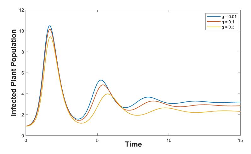
Figure 1: Impact of the variation of g in the number of infected plant population (difference not visible).
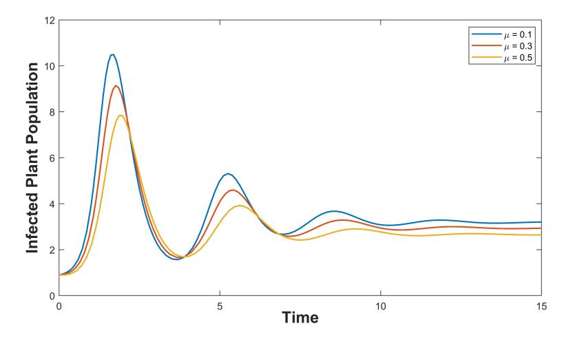
Figure 2: Impact of the variation of \(\mu\) in the number of infected plant population.
According to Routh-Hurwitz theorem, the endemic equilibrium \(T_2(S^*, I^*, P^*, R^*)\) is locally asymptotically stable if \(A_1>0, A_3>0, A_4>0\) and \(\Delta=A_1A_2A_3-A_3^2-A_1^2A_4>0\). Wei-Min Liu [28] introduced an equivalent condition for simple Hopf bifurcation without determining eigenvalues. According to the theorem by Liu, the endemic equilibrium \(T_2\) undergoes a simple Hopf bifurcation if
\[\begin{split} \mathbf{CH1}: & A_1(\theta^H), A_2(\theta^H), A_3(\theta^H), A_4(\theta^H) > 0 \quad \text{and} \quad \Delta(\theta^H) = 0, \\ \mathbf{CH2}: & \frac{d\Delta(\theta^H)}{d\theta} \neq 0. \end{split}\]
Considering \(\Delta\) as a function of \(\theta\), it is obtained that for the parameters in Table 4 with \(d_1=0.5\), at \(\theta=\theta^H\approx 0.805340\), \(\Delta=0\) (Figure 3). At the point \(\theta=\theta^H\approx 0.805340\), \(\frac{(d\Delta(\theta^H))}{d\theta}\approx -0.572197\neq 0\) (Figure 3). Also, \(A_1>0\), \(A_2>0\), \(A_3>0\), \(A_4>0\) at the point \(\theta=\theta^H\) (Figure 4). Hence conditions CH1, CH2 are satisfied and the disease-endemic equilibrium undergoes a simple Hopf bifurcation at \(\theta = \theta^H\). At \(\theta = \theta^H\), eigenvalues of the Jacobian matrix at the disease-endemic equilibrium are \(-0.874414, -0.110232, \pm 1.05103i\), which also confirms the existence of Hopf bifurcation. In Figure 5, the phase portraits are drawn for \(\theta = 0.78/day\) and \(\theta = 0.84/day\), which clearly depicts the existence of limit cycles.
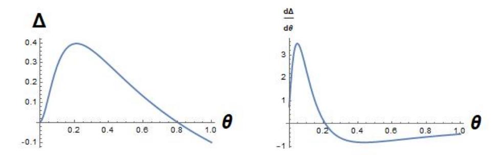
Figure 3: Plot of \(\Delta = A_1 A_2 A_3 - A_3^2 - A_1^2 A_4\) and \(\frac{d\Delta}{d\theta}\) as functions of \(\theta\) (Parameters are taken from Table 4).
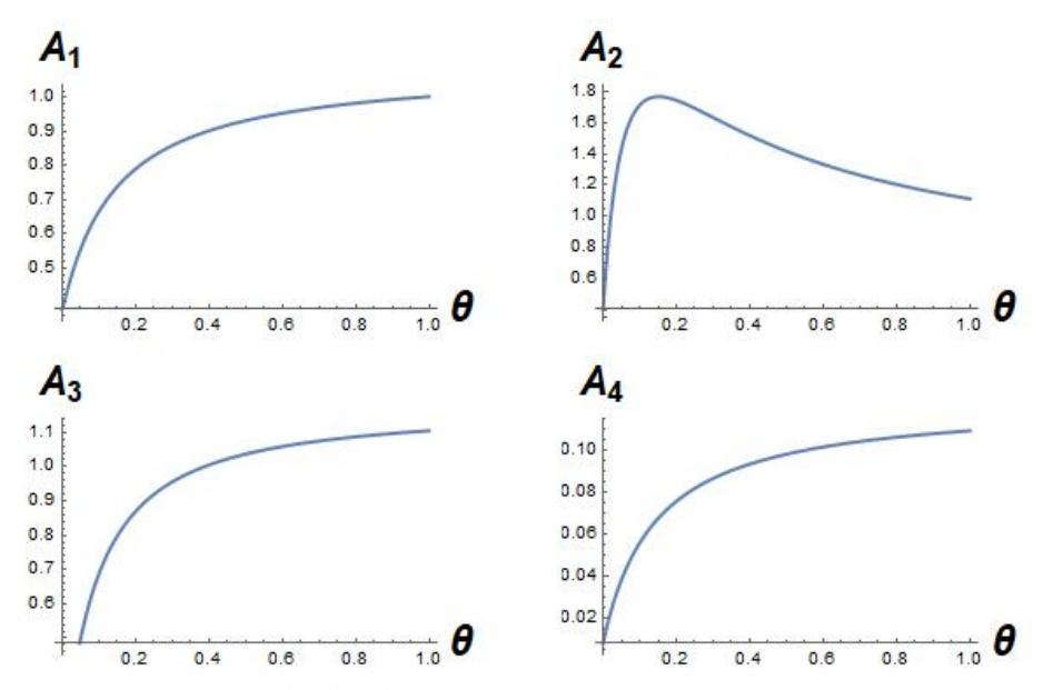
Figure 4: Plot of \(A_1\), \(A_2\), \(A_3\), \(A_4\) as functions of \(\theta\) (Parameters are taken from Table 4).
4. NUMERICAL SIMULATIONS
In this section, the proposed model is analysed numerically to observe the behaviour of the spread of disease and the role of control measures on the decline of the disease. Numerical analysis is done in MATLAB R2015a. For numerical simulations, we set S(0)=2, I(0)=0.9, R(0)=0.5 and P(0)=0.7 and the estimated values of parameters are shown in Table 4. It is observed that the trajectories of the system (1), initiating from the mentioned initial points, approach to the disease endemic equilibrium \(E^*=(8.3238,3.1797,7.9527,0.2891)\) (Figure 6). From Figure 6, it can be observed that initially the populations of the infected plants is dominant over the susceptible, but with an increase in the amount of pesticides use, the infected plants population
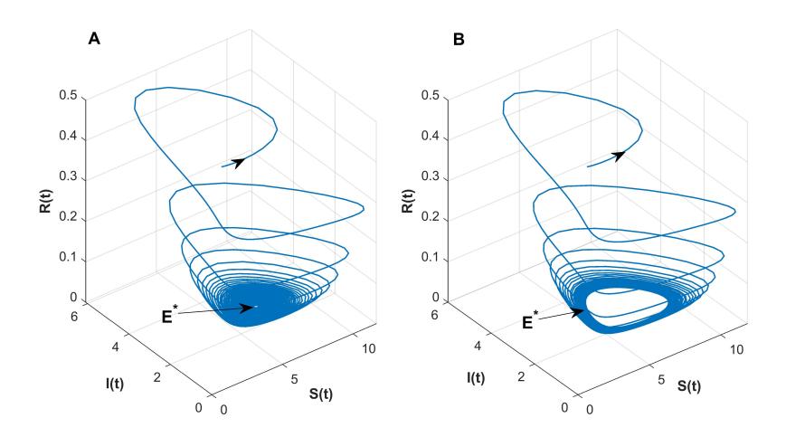
Figure 5: Phase portrait of the system 1 for \(\theta = 0.78/day\) and \(\theta = 0.84/day\) (other parameters are considered as mentioned in Table 4 with \(d_1 = 0.5\)).
Table 4: Parameter values used for Simulation.
| Variables | Definitions | Value |
|---|---|---|
| r | Intrinsic growth rate of the plant population | 3.5/day |
| k | Environmental carrying capacity | 25/ sq. meter |
| \(\beta\) | Contact rate between susceptible and infected plants | 0.3/ day |
| \(d_1\) | Contact rate between susceptible and pesticides | 0.1/ day |
| \(d_2\) | Contact rate between infected plants and pesticides | 0.3/ day |
| \(\mu\) | Death rate of plants due to pests | 0.1/ day |
| \(\nu\) | Rate of infected plants which have recovered and returned to the susceptible class | 0.01/day |
| g | Recovery rate of infected plants | 0.01/ day |
| \(\overset{\circ}{\theta}\) | Infective induce rate of pesticides | 0.5/ day |
| \(\alpha\) | Amount of pesticides used | 0.2/ day |
decreases with increase in time. Both the plant populations, after a certain time, become stable with the equilibrium state \(E^*\). For the same parameter set (Table 4) with \(d_1=0.5/day\), \(\theta=0.5/day\), the system 1 also have a disease endemic equilibrium \(\bar{E}^*=(4.4438,1.6229,4.0786,0.14832)\). Starting from the equilibrium \(\bar{E}^*\) we plot the curve of equilibrium using \(\theta\) as free parameter. The system (1) undergoes a supercritical Hopf bifurcation at \(\theta^H=0.805340/day\). The nature of the Hopf bifurcation is confirmed with the first Lyapunov coefficient, which is found to be \(-2.453621\times10^{-03}\). Starting from the Hopf point \(\theta^H\), we plot the Hopf bifurcation curve varying parameters \(\theta\) and \(\alpha\) (Figure 7), which leads to the detection of Generalised-Hopf (denoted as GH) and Bogdanov-Takens bifurcations (denoted as BT) at (\(\theta=0.818986\), \(\alpha=0.000470\)) and (\(\theta=0.825201\), \(\alpha=0\)) respectively. Near the point GH along the curve, the endemic equilibrium displays varying characteristics, transitioning from a supercritical to a subcritical state. This Hopf curve separates the \(\theta-\alpha\) space into stable and unstable. In the unstable region, all the populations of system (1) start oscillating periodically, i.e., the populations of the susceptible and infected plant oscillate periodically. In Figure 8, we represent the oscillatory, the susceptible populations is dominant over infected, i.e., the populations of the susceptible plant oscillates with a higher population than the infected.
Again, starting from the equilibrium point \(\bar{E}^*\), we compute the curve of equilibria with free parameter
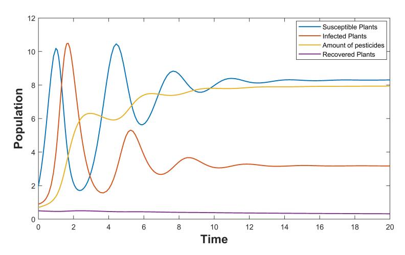
Figure 6: Time evolution of system (1) with the parameters mentioned in Table 4.
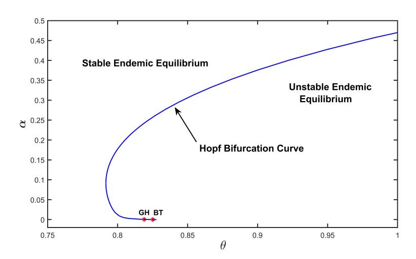
Figure 7: Two dimensional projection of Hopf bifurcation curve with free parameter \(\theta\) and \(\alpha\).
\(d_1\) which leads to a supercritical Hopf bifurcation at \(d_1^H=0.627463/day\), where the first Lyapunov coefficient is \(-2.227478\times 10^{-03}\). From this point \(d_1^H\), we compute the two-dimensional projection of Hopf bifurcation curve with free parameters \(d_1\) and \(d_2\) (Figure 9). Figure 9 represents a parametric region where the endemic equilibrium shows different stability. For the unstable region, the endemic equilibrium shows periodic oscillatory behaviour.
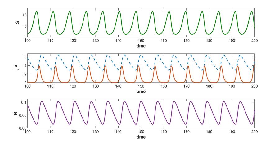
Figure 8: Time evolution of system (1) with the parameters mentioned in Table 4 and d1 = 0.5/day, θ = 1/day. The dotted line represents the amount of pesticides used.
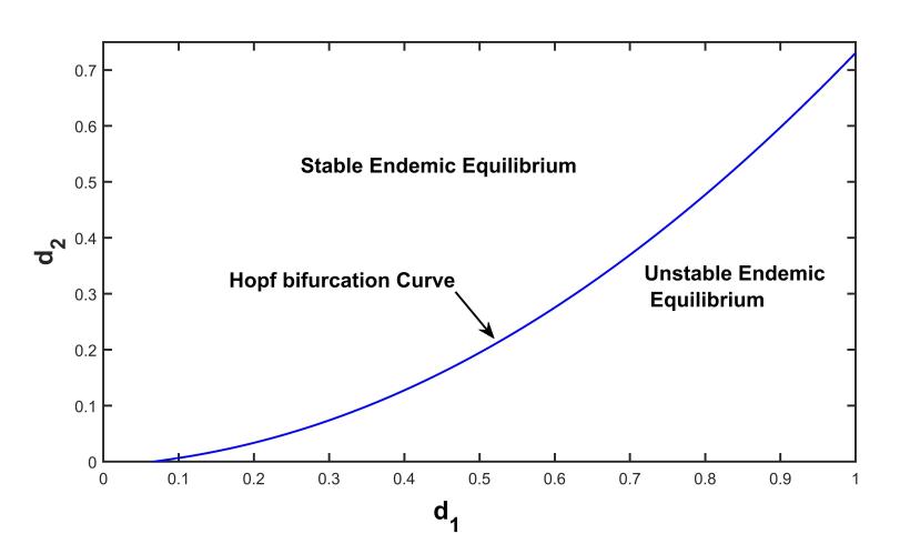
Figure 9: Two dimensional projection of Hopf bifurcation curve with free parameter d1 and d2.
5. CONCLUSION AND DISCUSSION
In this paper, we proposed and analysed a compartmental plant-pesticide model represented by a system of ordinary differential equations (ODEs). We divide the plant populations into three compartments: the susceptible, the infected, and the recovered population. As a control measure, pesticides are applied to all the plants to reduce disease transmission from infected to susceptible plants. We assumed that pesticides impact both the susceptible and the infected populations. The necessary mathematical analysis for the biological validity of the proposed model were presented first. The boundedness theorem (Theorem 3.2) implies that each plant population is bounded above for t → ∞. The total plant population N(t) is also bounded above whenever t → ∞, i.e., the system will not be collapsed due to population explosion. Uniqueness and the existence of solutions are one of the most important parts of mathematical modeling. In our model, unique solutions exist. If the solutions are not unique then there may exist two different equilibria, e.g., two different
diseases endemic equilibrium. In that context, different initial populations may lead to different equilibrium states. In our study, we also determined a domain in which solutions of the system exist. Our proposed system has three feasible equilibrium points. The first is the trivial equilibrium point \(T_0\), which always exists and is stable if \(r < \mu\). If \(r > \mu\) the equilibrium point \(T_0\) becomes unstable resulting the appearance of the disease free equilibrium (DFE) point \(T_1\) and the endemic equilibrium point \(T_2\). Using next generation matrix method, we determined the basic basic reproduction number \(R_0\) of the infection. Sensitivity analysis was carried out to understand the relation between basic reproduction number \(R_0\) and the associated parameters. Finally, we employed a biologically plausible set of parameters to perform numerical simulations, aiming to compare the analytical findings. Additionally, we employed numerical simulations to generate Hopf bifurcation curves in various parameter spaces. Summarizing our analysis, the results can be outlined as follows.
- 1) The disease-free equilibrium (DFE) is locally asymptotically stable whenever the basic reproduction number of the epidemic is less than unity. It signifies that the disease has been eradicated from the plants population. On the other hand, when the basic reproduction number exceeds unity, the DFE becomes unstable, indicating the presence of the disease in the plants population.
- 2) The endemic equilibrium is found to be locally asymptotically stable under specific conditions which can be obtained utilising the Routh-Hurwitz Criteria. For the provided parameters all the population coexists with an endemic equilibrium \(E^* = (8.3238, 3.1797, 7.9527, 0.2891)\).
- 3) The sensitivity indices of the basic reproduction number \(R_0\) are determined and the impacts of associated parameters have been analysed. \(R_0\) tend to change its value as the value of the associated parameter increases or decreases, and remain constant whenever the value of the associated parameters are constants. It is observed that the value of \(R_0\) increases as the value of r increases and the value of \(R_0\) decreases as the value of r increases and the value of r0 decreases as the value of r1 increases.
- 4) It is observed that initially, the population of infected plants predominates over the susceptible plants, but as the amount of pesticide increases, the infected plant population decreases over time (Figure 6). Both plant populations become stable after a certain period of time.
- The inner dynamics of the system for varying the infective induce rate of pesticides was also discussed. It was found that the endemic equilibrium undergoes a supercritical Hopf bifurcation at \(\theta = \theta^H \approx 0.805340\) i.e., above this critical parameter, all the population starts oscillating periodically and the equilibrium state becomes unstable.
- 6) With free parameter \(d_1\), the model leads to a supercritical Hopf bifurcation at \(d_1^H = 0.627463/day\). A parametric region in parameters \((d_1, d_2)\), where the endemic equilibrium shows different stabilities, is determined. For the parameters \(d_1\) and \(d_2\), above the curve (Figure 9), all the populations coexist within the ecosystem, while for parameters below the curve all the populations will start oscillating periodically. Hence an unstable ecosystem can be observed where populations will fluctuate, never tending to a stable state.
Previous studies in the literature have examined eco-epidemic models focusing on either prey or predator populations, where they are divided into susceptible and infected categories. However, this research emphasizes the plant populations undergoing an epidemic with a disease and is partitioned into susceptible and infected. Furthermore, to mitigate the epidemic, the application of pesticides is implemented, resulting in the recovery of plant populations. Plant epidemics have been documented in various cultivated plants like tea and pineapples, leading to significant revenue losses [26]. Rice is the most important economic crop in India, China, East-Asia, South East Asia, Africa and Latin America catering to nutritional needs of 70% of the population in these countries [13], [23]. Rice diseases caused by fungi are considered the main constraint in rice production and cause both qualitative and quantitative losses. In particular, rice blast disease caused by Pyricularia oryzae (Magnaporthe grisea) has been reported as the most significant disease, resulting in yield losses of up to 50%. Dirty panicle disease or rice grain discoloration may be caused by many fungi, viz., Alternaria padwickii, Curvularia lunata, Fusarium moniliforme, and Bipolaris oryzae. Propiconazole and Tricyclazole are often applied in rice crops as a prevention measure for these fungal diseases. Although they are not intended to harm non-infected rice plants, their residues and the risk of phytotoxicity underscore the potential consequences, which can vary and lead to plant fatality [22]. This instance is a suitable illustration for the proposed model, and the conclusions drawn rely entirely on analytical results. Experimental validation will indicate any required modifications to underlying assumptions.
The work in this paper can be extended to review several important crop epidemics. Also, there is a scope for using optimal control theory to optimise the cost-effectiveness of the system [12], [32]. The objective
will be to minimise the damage caused by the infected plant populations and the cost of application of pesticides as a control measure. Application of pesticides does not always give immediate recovery of the infected plants. There is a possible delay in the recovery process. Our studied model can be extended to a time-delay model using delay differential equations. Over the years, researchers have paid much attention to the studies of fractional order eco-epidemiological models as well [30], [10], [6]. This work can also be extended using fractional order derivatives. Furthermore, researchers with a keen interest can explore this model by examining contact rates between plants and pesticides, which are entirely dependent on the quantity of pesticides applied. This can be achieved through the utilization of functions that rely on the variable α.
ACKNOWLEDGEMENT
The authors would like to thank the editor and the referees for their valuable comments and suggestions that improved the quality of our paper.