

1. INTRODUCTION
Diabetes is a metabolic disorder with symptoms are insufficient insulin synthesis or inadequate insulin sensitivity. There are two types of diabetes: Type 1 and type 2 diabetes. The immune system targets the pancreatic β-cells that produce insulin when a person has type 1 diabetes. As a result, the pancreas cannot control blood glucose levels, resulting in nerve damage, blindness, and chronic renal dysfunction [1]. Type 2 diabetes is accompanied by reduced insulin efficiency to promote glucose transport into the cells and does not require insulin injections [2].
Patients with type 1 diabetes require daily exogenous insulin injections to overcome the lack of insulin and to stay alive. Diabetes diagnosis is based on a fasting blood glucose concentration above normal [3] So, a diabetic person should manually perform the procedures of blood glucose regulation. However, if a system existed that automatically monitors and controls blood glucose levels, diabetic patients could better operate their daily activities. Scientists and engineers have been working to create an artificial pancreas to automate the insulin control process. The controller transmits the input control to the artificial pancreas (insulin pump) to inject a specific insulin dose into a diabetic patient's blood based on the input, the blood glucose level obtained from a sensor [4].
This device includes a glucose concentration sensor, an infusion insulin pump, and a control algorithm. The normal range of blood glucose levels in individuals is 70-110mg. Food consumption, digestion rate, activity, and reproductive status are exogenous factors influencing blood glucose concentration levels. Some control algorithm [5], robust control [4], and sliding mode control [6] have all been presented as control algorithms for blood glucose regulation. The controller is designed to keep blood glucose levels within normal limits. A model-based technique calculates the insulin infusion rate with an updated controller.
∗Corresponding author
Received March 17th, 2023, Revised May 26th, 2023, Accepted for publication July 6th, 2023. Copyright ©2023 Published by Indonesian Biomathematical Society, e-ISSN: 2549-2896, DOI:10.5614/cbms.2023.6.2.1
Sliding Mode Control has attracted much attention in biological studies because of its unique characteristics, such as remarkable resilience, simplicity, and fast convergence rate [7]. The Sliding Mode Control considers a nonlinear sliding surface rather than a linear one. The selected surface acts as an attraction for the state trajectories. It is model-based, so a mathematical model of glucose-insulin dynamics is necessary to construct the controller [8]. However, glucose-insulin dynamics in the human body are intricate and involve nonlinearity, necessitating the identification of a significant number of model parameters. To deal with the higher order sliding mode strategies for regulating blood glucose in type 1 diabetic patients. A higher-order backstepping sliding mode control is designed for this structure, too [9]. Also, the super twisting control approach is studied and investigated the internal model sliding mode control for glucose regulation in type 1 diabetic patients [10].
The glucose regulation varies significantly from patient to patient and daily for the same patient. As a result, an accurate model is either unavailable, or the computing cost of an exact and dependable model needs to be revised. Numerous researchers have looked into model-based controllers, which use only input and output data in their design techniques [[4]-[8], [14], [16]]. Robust and adaptive control are two primary and complementary approaches to dealing with model uncertainty. The typical structure of a robust controller is composed of a nominal part and additional terms to address model uncertainty. An adaptive controller has a similar structure, but it updates the model based on the observed performance during operation. [15].
This work proposes a new way to control blood glucose in type 1 diabetes. Because the glucose-insulin system is a complicated nonlinear system, the model parameters fluctuate from patient to patient and are always subject to disturbances and uncertainty [2]. We proposed an adaptive sliding mode controller that aims to make the tracking error between actual blood glucose and references blood glucose go to zero. In other words, the controller is subject to decreasing the diabetic patient's high blood pressure to the reference condition, which is basal level.
This study is organized into five sections. Section 1 is about the introduction and objective of this study. In section 2, we give the mathematical model explanation. Section 3 will give the detailed adaptive sliding mode control theory. Then, the numerical simulation is given in Section 4. Moreover, the conclusion is given in Section 5.
2. MODEL FORMULATION
The mathematical model of the insulin dynamics in the blood plasma was proposed by [11] called the Bergman Minimal Model. In this research, we use the modified version from [12] and [13]. The model consists of a single glucose compartment, whereby plasma insulin is assumed to act as the "remote" compartment influencing glucose uptake. Bergman's minimal model is modified by adding a glucose infusion term \(U_a(t)\)which states the effect of glucose intake from a meal. The definition of compartments and parameters of the model are shown in Table 1 and Table 2. The flows of the glucose regulation given in Figure 1. The assumption of the models are [13]:
- The kinetics of glucose and insulin are described by decomposing the system into several discrete compartments.
- The effect of transmission between compartments is instant. The observed lag in glucose response to insulin levels was modeled using the "remote" insulin compartment X.
- All well-stirred compartments. That is, instantaneously, the plasma glucose concentration is always assumed to be uniform to the body over time.
The blood glucose regulation model given is as follows [12]:
\[\frac{dG}{dt} = -p_1 G(t) - X(t)(G(t) + G_B) + U_g(t), \tag{1}\]
\[\frac{dX}{dt} = -p_2X(t) + p_3I(t), \tag{2}\]
\[\frac{dG}{dt} = -p_1 G(t) - X(t) (G(t) + G_B) + U_g(t),\] \[\frac{dX}{dt} = -p_2 X(t) + p_3 I(t),\] \[\frac{dI}{dt} = -n(I(t) + I_B) + \frac{1}{V_L} u(t).\] (1)
For further, (1)-(3) will be called system (1). The Equation (1) describes the dynamics of plasma glucose concentration. The Equation (2) describes the dynamics of the transport of insulin from the blood to interstitial fluid. The Equation (3) describes the change of free plasma insulin concentration in the blood plasma. The term \(U_g(t)\) is the rate of infusion of exogenous glucose and u(t) is the rate of infusion of insulin. In other words, the term \(U_g(t)\) is the rate of exogenous glucose entering the blood from intestinal absorption after a meal defined. Different from [12], we use \(U_g(t)\) in the following formula [14]:
\[U_g(t) = \frac{D_G A_G t e^{\frac{t}{t_{max,G}}}}{t_{max,G}^2},\tag{4}\]
mg/dL
10 [1] where \(D_G\) is the number of carbohydrates digested, \(A_G\) is the carbohydrate bioavailability, and \(t_{(max,G)}\) is the interval between the start of a meal and when the absorption rate hits its maximum. We use the value of \(A_G = 0.8\) and \(t_{(max,G)} = 40\) minutes [14]. Therefore, Equation (4) can be written in the following form [1]:
\[U_g = \begin{cases} (0.025D_G(k - k_G)e^{(-0.125(k - k_G))}, & if k \ge k_G, \\ 0, & otherwise, \end{cases}\] (5)
where \(k_G\) is the time-step when the meal disturbance is given.
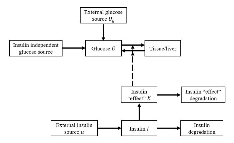
Figure 1: The Bergman Minimal Model (including insulin compartments applicable to the diabetic state). Solid lines represent 'flows' while the broken line represents a 'signal' which affects the tissue/liver compartment flow rates [13].
Compartment Description Unit Initial Value G The blood glucose concentration in the blood plasma mg/dL X The concentration of insulin in the remote compartment mg/dL X 0 [1]
The insulin concentration in the blood plasma
Table 1: Description of compartments.
3. SLIDING MODE ADAPTIVE CONTROL FOR BERGMAN MINIMAL MODEL
Model imprecision in a nonlinear system typically results from unknown system parameters or a purposeful choice to depict the dynamics of the system in a simplified form. Nonlinear control systems can suffer significantly from inaccurate modelling. Two primary and complementary methods for addressing model uncertainty are robust and adaptive management. A nominal part and additional terms intended to address model uncertainty make up the typical structure of a robust controller. Similar in structure, an adaptive controller updates the model based on measured performance while in operation [15]. In this paper, we will combine the two structures above as sliding mode adaptive control based on the study of [16] and [7].
| Parameter | Description | Unit | Value |
|---|---|---|---|
| \(p_1\) | The insulin-independent glucose-utilization rate | \(min^{-1}\) | 0 [1] |
| \(p_2\) | The rate of decrease of the tissue glucose uptake ability | \(min^{-1}\) | 0.028344 [14] |
| \(p_3\) | The insulin-dependent increase of the glucose uptake ability | mL/uU.min-2 | 5.0353×10⁻⁵ [14] |
| \(G_B\) | The steady state or basal plasma glucose | mg/dl | 120 [14] |
| \(I_B\) | The insulin levels under no external influences | mg/dl | 10 [14] |
| \(V_L\) | The insulin distribution volume | Ĺ | 12 [14] |
| n | The first order decay rate for insulin in blood | \(\mathrm{min}^{-1}\) | 0.1 [14] |
| \(U_g(t)\) | A disturbance (meal disturbance) input | mg/dl.min-1 | |
| u(t) | The infusion rate of the exogenous insulin | mU/min |
Table 2: Description of parameters.
3.1. Sliding Mode Control Design
The sliding mode control consists of two phases: reaching and sliding. In the reaching phase, the state trajectory moves the sliding surface forward. While in the sliding phase, the state trajectory is directed to move forward the origin along the sliding surface [7]. In this subsection, sliding mode control is proposed for the blood regulation model in the system (1) to decrease the high-blood pressure of type I diabetic patients and bring it to the basal level \(G_B\) while handling the parameter uncertainty. Define the tracking error as follows:
\[e_r(t) = (G(t) - G_r e f(t)) + (I(t) - I_r e f(t)),\] (6)
where G(t) is the glucose concentration in the blood plasma at time t, \(G_{ref}(t)\) is the reference function (signal tracking reference) for G(t), I(t) is the insulin concentration in free blood plasma at time t, and \(I_{ref}(t)\) is the reference function (signal tracking reference) for I(t) that satisfy:
\[G_{ref}(0) = G(0), \tag{7}\]
\[G_{ref}(t) = G(0), \tag{7}\] \[(G_{ref}(t) - G_{tf}) \to 0, t \to \infty, \tag{8}\] and
\[I_{ref}(0) = I(0),\] (9)
\[(I_{ref}(t) - I_{tf}) \to 0, t \to \infty. \tag{10}\]
Equations (7) and (9) states that the initial condition of tracking error is zero, \(e_r(0)=0\). Equation (8) states that the reference function G(t) asymptotically goes to the normal blood pressure target \(G_{tf}\). In contrast, Equation (10) states that the reference function I(t) asymptotically goes to \(I_{tf}\), the basal level \(I_B\). The reference function is freely proposed based on the control objective as long as desired Equations (7)-(10). The control objective of this work are decrease the high level of blood glucose of the diabetic patient type I and keep it remind in the basal level. So, we choose the exponential function to capture the decreasing of the blood glucose as the reference function [12] as follows:
\[G_{ref}(t) = (G(0) - G_{tf})e^{(-\xi t)} + G_{tf},\] (11)
\[I_{ref}(t) = (I(0) - I_{tf})e^{(-\xi t)} + I_B,\] (12)
where parameter \(\xi > 0\) is the convergence rate of the reference function curve, G(0) is the initial concentration of blood glucose in the blood plasma, \(G_{tf}\) is the target blood glucose concentration at the end of the simulation, I(0) is the initial concentration of insulin in the remote compartment, and \(I_{tf}\) is the target concentration of insulin remote at the end of the simulation. The sliding mode controller consists of two terms, that is the equivalent control \(u_{eq}\) and the switching control \(u_{sw}\). While the switching control forces the system in the direction of the sliding surface, the equivalent control maintains the system's position on the sliding surface. Defined the sliding variable \(\sigma(t)\) that satisfies:
\[\sigma(t) = e_r(t). \tag{13}\]
The sliding surface that guarantees the control objective will be achieved is given by:
\[\sigma(t) = e_r(t) = 0. \tag{14}\]
In order to preserve the states to remain on the sliding surface, the equation must hold σ(t) = σ(t) = 0. The time derivative of the sliding variable gives
\[\dot{\sigma}(t) = \dot{e}_r(t) = \dot{G}(t) - \dot{G}_{ref}(t) + \dot{I}(t) - \dot{I}_{ref}(t) = \dot{G}(t) + \xi(G(0) - G_{tf})e^{(-\xi t)} + \dot{I}(t) + \xi(I(0) - I_{tf})e^{(-\xi t)},\] (15)
by substituting σ(t) = 0 to Equation (15), we obtained the control u called the equivalent control as follows,
\[u_{eq}(t) = V_L \left[ p_1 G(t) + X(t) G(t) + X(t) G_B - U_g(t) - \xi(G(0) - G_{tf}) e^{-\xi t} + n(I(t) + I_B) - \xi(I(0) - I_{tf}) e^{-\xi t} \right].\] (16)
The uncertainty makes the system exactly unknown. Therefore, we used the nominal parameter and defined it as follows,
\[\hat{p}_1 = (1 + unc)p_1,\] (17)
\[\hat{n} = (1 + unc)n, \tag{18}\] where pˆ1 is the nominal parameter of p1, nˆ is the nominal parameter of n, and unc is the uncertainty factor. As a result, the equivalent control becomes
\[\hat{u}_{eq} = V_L \left[ \hat{p}_1 G(t) + X(t) G(t) + X(t) G_B - U_g(t) - \xi(G(0) - G_{tf}) e^{-\xi t} + \hat{n}(I(t) + I_B) - \xi(I(0) - I_{tf}) e^{-\xi t} \right].\] (19)
Since the equivalent control operates by assuming that the sliding surface is reached, using it in the system (1) may not achieve the control aims. Hence, the equivalent control Equation (19) be enlarged non-linearity to achieve robustness by opted the switching control in the term of the constant rate [7] as follows:
\[u_{sw}(t) = g(x, t)sgn(\sigma(t)), \tag{20}\]
where g(x, t) is gain switching, and sgn(x) is the signum function. Therefore, the controller becomes
\[u(t) = \hat{u}_{eq}(t) + u_{sw}(t), \tag{21}\]
where ueq(t) is in Equation (19) and usw(t) is in Equation (20).
Gain switching g(x, t) is defined based on the following assumptions [16]:
Assumption 1. There is a state-dependent function b(x, t) such that the following upper bound satisfy:
\[|(p_1 - \hat{p}_1)G(t) + (n - \hat{b})I(t)| \le b(x, t), t \ge 0.\] (22)
Assumption 2. The upper bound of b(x,t) is known.
Assumption 3. Gain switching g(x,t) has opted as follows:
\[g(x,t) = b(x,t) + \eta, \tag{23}\]
where η > 0 arbitrary.
Assumption 1 is linked to the maximum uncertainty due to unknown parameters. The function b(x, t) always exists as long as a particular parameter will parameterize the model, although the value is unknown. The typical assumption for the sliding mode control is Assumption 2, which states that the upper bound of the system is precisely known [15]. Assumption 3 defines the selection of the switching gain g(x, t). Further, Assumption 2 will be impaired by online adaptation of switching gain g(x, t) that removes a prior knowledge on the system's parameter or their bounds. Next, Theorem 3.1 (modified from [7]) will be proven.
Theorem 3.1. Given the Bergman minimal model (1)-(3) with control law (21). If assumptions 1, 2, and 3 are satisfied, then the error tracking er(t) vanishes asymptotically.
Proof: We will proof the theorem by using the Lyapunov stability theorem. Consider the following Lyapunov candidate function:
\[V(t) = \frac{1}{2}\sigma^2(t). \tag{24}\]
Time-derivative of (22) is calculated as
\[\dot{V}(t) = \sigma(t)\dot{\sigma}(t) = \sigma(t)(\dot{G}(t) + \xi(G(0) - G_{tf})e^{(-\xi t)} + \dot{I}(t) + \xi(I(0) - I_{tf})e^{(-\xi t)} = \sigma(t)(-p_1G(t) - X(t)G(t) - X(t)G_B + U_g(t) + \xi(G(0) - G_{tf})e^{(-\xi t)} - n(I(t) + I_B) + \frac{1}{V_L}u(t) + \xi(I(0) - I_{tf})e^{(-\xi t)}) = \sigma(t)((p_1 - \hat{p}_1)G(t) + (n - \hat{n})I(t) - g(x, t)sgn(\sigma(t))) \leq \sigma(t)(b(x, t)sgn(\sigma(t)) - g(x, t)sgn(\sigma(t))) = \sigma(t)(-ksgn(\sigma(t))) = -k|\sigma(t)| \leq 0.\] (25)
Based on assumptions 1, 2, and 3, the time derivative of V (t) for V (t) ̸= 0 is negative definite. Hence, based on the Lyapunov stability theorem [17], the origin σ(t) = 0 asymptotically stable, so that σ(t) → 0 as t → ∞ In other words, the sliding mode controller leads the error tracking to zero asymptotically.
Further, G(t) → Gref (t) as t → ∞ and I(t) → Iref (t) as tß∞ so that the blood glucose will go through the normal condition. Theorem 3.1 guarantees that the sliding mode controller can satisfy the control objective: decrease the high blood glucose and bring it to the basal condition. On the other hand, one of the lacks of this approach is that the switching gain in Assumption 3 is defined by the upper bound b(x, t), resulting in the function b(x, t) must be known precisely (Assumption 2). In some cases, it is challenging to obtain b(x, t) due to the complexity of the proposed controller. Therefore, the switching gain will be online adaption to avoid a priori knowledge in the upper bound of the controller.
3.2. Adapting Switching Gain of Sliding Mode Control
The switching gain g(x, t) in Equation (23) will be online adaption to avoid a priori knowledge of the upper bound of b(x, t) in Assumption 2. Assumption 4 below is the expansion of Assumption 1 to prove the stability of the proposed controller.
Assumption 4. [16] There is a finite constant, potentially unknown, positive b such that b ≥ b(x, t).
While Assumption 4 asserts that the function is bounded by a constant, Assumption 1 asserts that the higher bound is a state-dependent function. According to this assumption, the absolute difference between the nominal and actual parameter is constrained by a constant from a biological standpoint. It should be noted, though, that the upper limit may only be used to prove stability and may not be explicitly known during the control design process. Besides, adaptation switching gain starts at zero and rises until the sliding condition is met. The switching gain (23) changed into
\[\hat{u}_{sw}(t) = \hat{g}(t)sgn(\sigma(t)). \tag{26}\]
As a result, the proposed controller u in Equation (21) changed into
\[u = V_L[\hat{p}_1G(t) + X(t)G(t) + X(t)G_B - U_g(t) - \xi(G(0) - G_{tf})e^{(-\xi t)} + \hat{n}(I(t) + I_B) - \xi(I(0) - I_{tf})e^{(-\xi t)}] + V_L\hat{g}(t)sgn(\sigma(t)),\] (27)
where it is time-varying switching gain updated by this following equation:
\[\frac{d\hat{g}}{dt} = \Gamma \sigma(t) sgn(\sigma(t)) = \Gamma |\sigma(t)|, \hat{g}(0) = 0, \tag{28}\] where Γ a positive constant.
The switching gain gˆ(t) may be divergence due to the difference in Equation (19) being definite nonnegative over time. The critical point that guarantees that the error tracking goes to zero is the positive
constant b in Assumption 4, although the value is unknown. Therefore, the switching gain will rise until it reaches the upper bound b ≥ b(x, t). Then the system will converge to the sliding surface, and the sliding condition is achieved, σ(t) = 0, which stops the increasing switching gain. This schema meets the objective control such as Proposition 3.1. below apply.
Proposition 3.1. Given the Bergman minimal model in system (1) with the controller (19) and (20). If Assumptions 1 and 4 are satisfied for a finite upper bound b that may be unknown and Γ > 0, then the tracking error er(t) goes to zero asymptotically.
According to theory, the adaptive sliding mode control lowers blood glucose in the blood plasma while maintaining normal pressure and overcoming uncertainty.
4. SIMULATION
In this section, we simulate the dynamics of the blood glucose system based on the proposed controller. The initial condition and parameter value are given in Table 1 and Table 2. The initial value of G(0) = 225 mg/dL is chosen represents the condition of type 1 diabetes patients with hyperglycemia, namely blood glucose levels above 180 mg/dL. For diabetic (glucose resistant) subjects, the value of p1 is significantly reduced and so for theoretical simulation we use p1 = 0 [12]. The meal disturbance Ug is given three times at mealtime: breakfast time at 7 a.m., lunch at noon, and dinner at 7 p.m., and the value of DG is assumed to vary based on the mealtime. The DG value is the corresponding meal sizes of carbohydrates. It is assumed that the portion of meal consumption are different between breakfast, lunch, and dinner [1]. We use DG = 60 for breakfast, DG = 80 for lunch, and DG = 70 for dinner. So, Equation (5) becomes:
\[U_g = \begin{cases} 0.025(60)(t - 120)e^{(-0.125(t - 120))}, & t \le 120, \\ 0.025(80)(t - 420)e^{(-0.125(t - 420))}, & 120 < t \le 420, \\ 0.025(70)(t - 840)e^{(-0.125(t - 840))}, & 420 < t \le 840. \end{cases}\] (29)
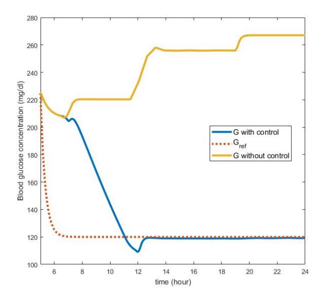
Figure 2: The blood glucose concentration (mg/dL).
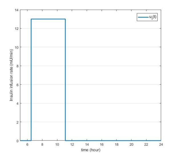
Figure 3: The Insulin infusion rates u(t).
The parameter value of switching gain is H = 0.0005, ξ = 0.05, and unc = 5%. For simulation purposes, we choose the upper bound of the controller umax = 13 mU/ml, which gives the best result of dynamics of the blood glucose simulation. We use the final target Gtf = GB = 120 mg/dl and Itf = 0. The simulation is over 24 hours, and the initial time is 5 a.m. The simulation result is shown in Figures 2-5. A brief comparison of the control strategy given in Table 3. The amount of control effort given can be seen in Figure 3.
Figure 2 shows the concentration of blood glucose levels without and with control efforts. In the uncontrolled condition, type I diabetes patients with initial blood pressure upon waking of 225 mg/dL (hyperglycemic) will experience an increase with every food intake (meal disturbance).
After having breakfast at 7 a.m., his blood pressure rose from 220 mg/dL to 234 mg/dL, then remained constant until just before lunchtime. After lunch at noon, his blood pressure rose again to 263 mg/dL, remaining constant until just before dinner. After dinner at 7:00 p.m., his blood pressure rose again to 281 mg/dL at 9:00 p.m. In contrast, after being given control through regular insulin injections, the patient's blood pressure can drop and be in the range of 100 – 120 mg/dL, which is normal. After breakfast at 7:00 a.m., the patient's blood glucose level decreased from 204 mg/dL to 120 mg/dL at 10:11 a.m. Blood pressure continued to drop until it reached 97 mg/dL at lunchtime. After lunch, blood pressure increased to 109.4 mg/dL at 13.00 and remained constant until just before dinner. Even so, the increase is still within normal blood pressure limits. After dinner at 19:00, blood pressure rose again until it reached 118.8 mg/dL at 19:36 and remained constant until the end of the simulation. These conditions indicate that control efforts have succeeded in reducing the blood pressure of hyper-glycemic patients and bringing them towards the control objective, namely the basal condition of GB.
Figure 3 shows the insulin infusion rates over 24 hours. Based on Figure 3, during the 24 hours of simulation, the insulin injection was given 30 minutes before breakfast, from 6:30 until 11 o'clock, with a maximal dose of injection is 13 mU/min. Whereas, apart from that time, insulin injection is not given. By applying that control strategy, the dynamics of the blood glucose level can be seen in Figure 2. Figure 5 shows that the error goes to zero at the end of the simulation, indicating that the control objective is achieved. As a result, the sliding surface σ(t) = 0 is also reached, and the switching gain gˆ(t) stop moving, as in Figure 5. It confirm the theoretical analysis in section 3 above.
Table 3: The comparison of the patient's blood glucose level over 24 hours.
| Condition | 7 a.m. (Breakfast) | 12 a.m. (Lunch) | 7 p.m. (Dinner) |
|---|---|---|---|
| Without control | 220 mg/dL | 234 mg/dL | 263 mg/dL |
| With sliding mode adaptive control | 204 mg/dL | 109.4 mg/dL | 118.8 mg/dL |
| Reduction | 7.27% | 53.25% | 54.83% |
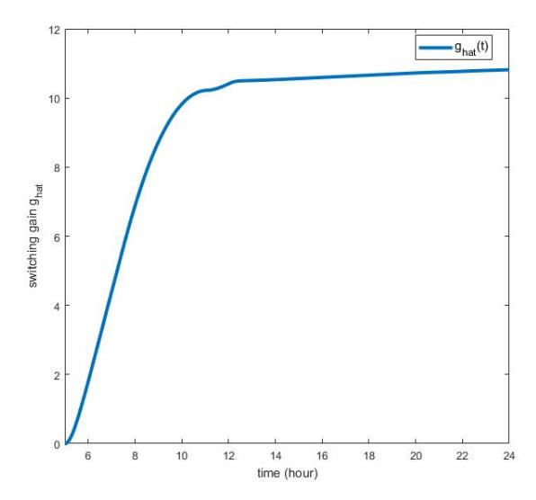
Figure 4: The adaptive switching gain gˆ(t).
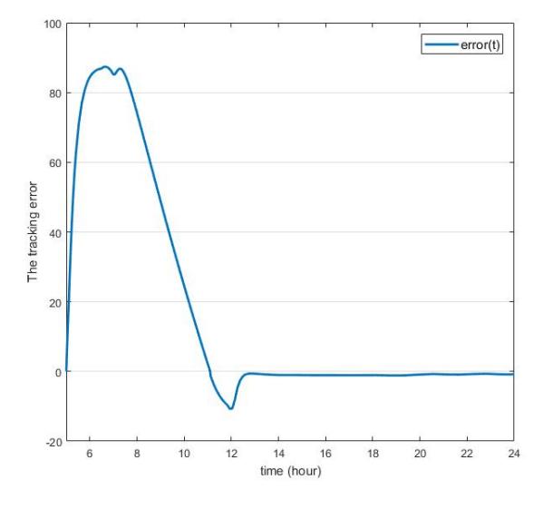
Figure 5: The tracking error er(t).
5. CONCLUSION
Adaptive sliding mode control successfully lowers the high blood glucose level in type 1 diabetic patients with hyperglycemic. The proposed controller can lower the patient's high blood pressure, maintain it in the neighbourhood of the normal glucose level, and reach the basal value GB at the end of the simulation. Based on the numerical simulation, to lower the high blood glucose in the hyperglicemic patient, the insulin injection should be given starting at 30 minutes before breakfast for the next four hour, with a maximal dose of injection is 13 mU/min. It can decrease the high blood pressure until 54.83%. For further research, the model should involve aspects of disturbance originating from external factors other than a meal disturbance.