

1. Introduction
1.1. Dengue fever
Globally, around 390 million cases of dengue, 500,000 hospitilisations, and 20,000 dengue related deaths are reported annually [1]. Dengue fever is a mosquito-borne viral-disease primarily transmitted by the Aedes aegypti mosquito, with the Aedes albopictus mosquito being the second most prevalent carrier of the disease [2], [3]. Over 125 countries are affected by the disease, and with international travel on the rise, the potential for infected travellers to unwittingly spread the disease further across the globe increases as well [4]. In Malaysia alone, in 2018, there were 80,615 new cases and 147 deaths attributed to the disease [5]. In 2010, the cost of the Malaysian dengue vector control program was 73.5 million USD [6]. Dengue fever is generally not fatal, although in some cases it can develop into a more serious, potentially life threatening, form called dengue haemorrhagic fever (DHF). Thus, due to huge financial and health implications, it has become a priority for health organisations worldwide to find a more efficient way of eliminating the dengue threat.
In the past, no dengue vaccine was available, so the only course of treatment was simply to treat the symptoms of infected patients, possibly combined with vector control. More recently, the first ever dengue vaccine was released in 2015. Unfortunately there are still some complications with its use, and for whom it is effective, and so it has not yet been widely adopted [7].
*Corresponding author
Received September \(5^{th}\), 2023, Revised October \(3^{rd}\), 2023, Accepted for publication October \(14^{th}\), 2023. Copyright ©2023 Published by Indonesian Biomathematical Society, e-ISSN: 2549-2896, DOI:10.5614/cbms.2023.6.2.7
Figure 1: A simplified illustration of the Mosquito Home System. Mosquitoes are attracted by the special solution (blue), enter the trap through the small (orange) openings at the top, and lay their eggs on the solution-soaked tissue paper near the bottom (yellow). A reservoir of solution is contained in an easily replaceable bottle that screws into the MHS, and feeds the pool at the bottom of the container with fresh solution, as the existing pool evaporates.
1.2. Control methods
Dengue spreading Aedes aegypti mosquitoes like to lay their eggs in dark, artificial containers, containing water, such as plant pots, flower vases and even discarded car tyres [8]. Ideal breeding sites contain a source of still, clean water, as well as a nearby source of blood to feed upon. Thus, built up, urban, human environments represent the perfect breeding ground for these mosquitoes [9].
Recent years have seen a shift in tactics used to combat mosquito-borne diseases around the world. Classical mosquito control methods, such as chemical fogging (or space-spraying) with pesticides, are very effective short-term, and produce rapid decreases in adult mosquito populations. However, fogging fails to affect newly laid mosquito larvae, which remain protected underwater, so long-term effects are minimal [10], and larvae readily replace every adult mosquito killed. In addition, fogging is generally only carried out once a case of dengue has already been reported, so it cannot stop an outbreak before it begins. Concerns about the evolution of pesticide resistant mosquitoes and potential negative health effects of the chemical sprays on humans are also growing [11]. Combined, these factors have driven an increase in research focussing on alternative mosquito control methods.
The new focus has been upon ways to eliminate mosquito larvae, before they develop into adult mosquitoes. Such techniques generally revolve around some form of modified ovitrap that will be lethal to either the adult female mosquito [12], or the newly laid larvae deposited within the trap.
1.3. The Mosquito Home System
The Mosquito Home System (MHS) is a novel design of ovitrap, see Figure 1. Classed as an autodissemination trap [13], it consists of an ovitrap type container, containing a solution that attracts ovipositing female mosquitoes, and a strip of tissue paper, upon which they can lay their eggs. A reservoir of solution is contained within an easily replaceable bottle in the centre of the trap, slowly drip feeding fresh solution into a pool at the base of the container at the same rate as the existing pool is evaporating. The solution contains an insect growth regulator (pyriproxifen) that is toxic to the mosquito larvae, but not the adults, and so any eggs that are laid within the trap are completely killed off [14]. In addition to killing the larvae, the female mosquitoes become contaminated with solution, which they may then transfer to nearby hidden breeding sites. This, in turn, kills off any eggs that are laid in hidden sites as well, hence the terminology "auto-dissemination", as the mosquitoes distribute the toxic solution among various local breeding sites.
Standard ovitraps have been used for years as a tool to monitor mosquito populations in a given area. They consist of a small dark container, containing water, and a substrate on which mosquitoes can lay their eggs. The eggs then fall off the substrate, through a mesh, into the water below. The eggs eventually hatch and grow into adult mosquitoes, but are trapped below the mesh and cannot escape. The trapped mosquitoes may then be counted, to estimate the local mosquito population size. These traps are one of the methods used to obtain the mosquito population data used later in this paper.
1.4. Outline of paper
In what follows, an outline of previous MHS field studies is provided, alongside general results from these trial locations. A novel hybrid deterministic-stochastic model is then presented, that simulates the effect of deploying the MHS within a built-up, residential, urban environment. Results from a series of test cases are presented to validate the model predictions against real-world data, and predictions from an existing deterministic model. The stochastic model provides unique insights into the effect of the MHS on dengue dynamics within a block of flats, and also allows the distribution of all possible outcomes for a given parameter set to be predicted. Results clearly suggest that the MHS significantly limits the potential for large numbers of the flat residents to become infected. Similar investigations are carried out for the endemic equilibrium of dengue within the flats. Concluding remarks and limitations are highlighted at the end. This model can become a valuable tool for predicting the impact of the MHS, and help dengue control experts worldwide formulate effective strategies for deploying traps at new locations.
2. BACKGROUND
2.1. Selangor flats — MHS field study
In 2014, a 44 week trial of the MHS was conducted within three blocks of high-rise flats that make up the Ridzuan Court Sunway in Selangor, Malaysia. This is a densely populated area within the Klang Valley, which is centred in Kuala Lumpur, and responsible for around 60% of the dengue cases of Malaysia [15] and was declared a dengue hotspot at the end of 2013. Combatting dengue within the flats has proven very difficult via conventional control methods, and so this made it an ideal location to trial the MHS [16].
Each of the three blocks is 26-27 storeys high, with ten units on each floor, occupying a floorspace of approximately \(7,500 \, \mathrm{ft}^2\) on each level [14]. There are in total 800 housing units, across the three blocks, and 3,200 residents, if we assume that each house has an average of four occupants. Originally four MHSs were deployed per floor, in each of the three blocks of flats. After the first 12 weeks, an additional eight MHSs per floor were added to one of the blocks of flats which appeared to have a significantly larger mosquito population than the other two. This brought the total number of MHSs to \(552 \, [14], \, [16].\)
During the 2014 trial, only 13 dengue cases were reported within the flats. This was a significant reduction, compared to 53 confirmed cases for the same period in 2013, and 57 cases in 2015 once the MHSs were removed [14]. The trial noted that the mean number of eggs laid in each MHS decreased as the trial progressed, with the mean decreasing by around 70.65% for one block of flats in particular [16].
Full results of the field study can be found in [16], whilst an existing deterministic model of the MHS within the same blocks of flats can be found in Greenhalgh et al. [17]. Results from the deterministic model will be used alongside the field study data, to help validate the new stochastic model presented below.
2.2. Singapore Botanic Gardens Trial
Another trial of the MHS was conducted at the Jacob-Ballas Childrens' Park in the Singapore Botanic Gardens from December 2015 – January 2016. This concluded that the introduction of the MHS traps led to a 58.89% reduction in the Aedes mosquito population within the area [18]. The trial also found that the MHS traps were twelve times more attractive than standard ovitraps to mosquitoes laying eggs.
2.3. Statistics for Kuala Lumpur
The population of Kuala Lumpur in 2013 was approximately \(N_{H_1}=1,720,000\) [19]. The human and mosquito death rates, \(\mu_H\) and \(\mu_V\), can be approximated from existing data, and are simply the reciprocal of the average life expectancy of each species. In 2015 the average life expectancy in Malaysia was 75 years [20], whilst the average lifespan of an Aedes mosquito is 2 weeks [21]. Thus, \(\mu_H=1/(75\times365)=3.653\times10^{-5}~{\rm day}^{-1}\) and \(\mu_V=1/14=7.143\times10^{-2}~{\rm day}^{-1}\).
In 2013, the annual incidence rate of new, symptomatic, dengue cases in Kuala Lumpur was 150.2 per 100,000 [22]. In the period from 1995 to 2012, the total number of cases in Malaysia was approximately 505,264, with Kuala Lumpur responsible for around 3-10% of these [23]. In addition to obvious, symptomatic cases, dengue causes asymptomatic infections, which show no symptoms and are not counted. The literature disagrees on the ratio of symptomatic to asymptomatic cases. The ratio 1:3 is often cited, however this figure varies from 1:1 all the way up to 1:18 [24]. In what follows, this ratio is assumed to be 1:4 [25], [26], such that, for every symptomatic person, another four are asymptomatic. Thus, assuming 5% of dengue cases in Malaysia are from Kuala Lumpur, the total number of people that had recovered from dengue, in Kuala Lumpur in 2013, is estimated at 126,316 (= \(0.05 \times 5 \times 505,264\)).
3. MODEL FORMULATION
The mathematical model consists of two sets of six differential equations that simulate the dengue dynamics within the flats. The first set takes a deterministic approach to model the disease in the wider population of Kuala Lumpur, whilst the second set adopts a stochastic approach to evolve the same dynamics within the flats themselves. Both of these sub-models are outlined separately below.
3.1. The Ross-MacDonald approach
A set of deterministic, Ross-MacDonald style differential equations are used to evolve the human and mosquito population dynamics across the whole of Kuala Lumpur. The information from these is then fed into the stochastic model for the flats.
Developed over a seventy year period, the Ross-Macdonald equations are one of the most established approaches to modelling vector-transmitted diseases mathematically, and take the form of a Susceptible-Infected-Recovered (SIR) model [27]. The model divides the human population within Kuala Lumpur into three groups: Susceptible humans who are at risk of becoming infected with dengue; infected humans who are currently infected with the disease; and recovered humans who have now recovered from the disease. These three groups will be denoted \(S_{H_1}(t)\), \(I_{H_1}(t)\) and \(R_{H_1}(t)\), respectively, with the subscript "1" being used to specify that these represent the populations in Kuala Lumpur. Later, the subscript "2" will be introduced to represent the same populations within the block of flats, as outlined in Table 1. Using this model, it is assumed that once recovered, humans become immune until they die.
The mosquito population in Kuala Lumpur is also divided into three different groups. These are \(S_{V_1}(t)\), the number of susceptible mosquitoes; \(L_{V_1}(t)\), the latent mosquitoes; and \(I_{V_1}(t)\), the infectious mosquitoes. It is assumed that mosquitoes may become infected by biting an infected human, and if they do, then there is an incubation (latent) period of length \(\tau\) days before they themselves become infectious. Once infected, it is assumed that a mosquito is infected for life, until it dies.
Table 1: The main model variables. The subscript j distinguishes between the wider population in Kuala Lumpur and that in the flats: For example, \(S_{H_1}(t)\) denotes the number of susceptible humans in Kuala Lumpur, whilst \(S_{H_2}(t)\) denotes the susceptible humans in the flats. In general j=1 denotes Kuala Lumpur and j=2 represents the flats.
| Variable | Description | Variable | Description |
|---|---|---|---|
| \[\begin{array}{c} S_{H_j}(t) \\ I_{H_j}(t) \\ R_{H_j}(t) \\ N_{H_j} \end{array}\] | Susceptible humans Infected humans Recovered humans Total no. humans | \(S_{V_j}(t) \ L_{V_j}(t) \ I_{V_j}(t) \ N_{V_j}\) | Susceptible mosquitoes Latent mosquitoes Infected mosquitoes Total no. mosquitoes |
Deterministic models are generally the first approach adopted when modelling a new epidemiological scenario. This is usually due to their ease of implementation and their low computational expense [28]. They produce the same results each time, since the future state of the system has no dependence upon random events (like those found in a stochastic model). However, since the spread of dengue is dictated by a series of random events in nature, a stochastic approach is a better representation of reality. This is especially true when modelling smaller population sizes, as it is entirely possible that the disease may randomly become extinct due to the much smaller numbers infected at any one time [29].
Provided the population is large, however, a deterministic approach gives a good approximation to the more realistic results of a stochastic model [30], [31]. Subsequently, the deterministic approach is perfect for modelling the wider population across Kuala Lumpur. In general, we expect that the average results from a large number of stochastic simulations will tend towards the deterministic results when modelling the same situation. This convergence to the deterministic results is later used to examine the predictions of the new stochastic model. The models assume that the population is homogeneous; an assumption that may not hold true if super-infectors or super-connected individuals are present.
3.2. The stochastic model approach
During mosquito season, the mosquito population will be high within both the flats and Kuala Lumpur. However within the flats themselves, the number of both infected humans and infected mosquitoes will be very small (typically no more than 2 of each at anyone time). Thus it is more appropriate to adopt a stochastic model to evolve the population dynamics within the three blocks of flats. Within the literature, deterministic models are used far more commonly than stochastic models. Of the few stochastic dengue models that do exist, the Skeeter Buster tool by Magori et al. [32] is perhaps the most thorough that is currently available. Their model keeps track of the entire life history of mosquitoes, incorporating stochastic events, spatial heterogeneity and mosquito genetics, to predict mosquito dynamics at distinct locations (individual houses). Another approach is discussed by Samat and Percy [33], where they incorporate a Poisson-Gamma process into a stochastic SIR model to map the relative risk of dengue, on a state-by-state basis, for all 16 states in Malaysia. The numerical analysis of an SEIR (Susceptible, Exposed, Infectious, Recovered) type model for dengue can be found in Raza et al. [34], whilst Otero and Solari [35] present a minimalistic stochastic SEIR model, incorporating seasonality and spatial vector dynamics, to estimate the risk of a dengue epidemic in Buenos Aires, Argentina. However, none of these existing models incorporate the effects of mosquito traps, or other vector control solutions.
The stochastic approach is generally far more versatile than the deterministic equivalents, as it can be used to address questions such as the probability of epidemic fade out, as well as predict both the distribution and variance of the total number of cases that may occur. One of the key benefits of the stochastic model, is its unique ability to account for all possible scenarios when dengue is introduced to the flats, resulting in a distribution of all possible outcomes. This allows the aleatory (or intrinsic random) uncertainty to be estimated, and the effects of epistemic uncertainty (the uncertainty in the model assumptions or parameters) to be evaluated, whereas a deterministic model allows only the effects of the epistemic uncertainty to be evaluated. Overall, the output from the stochastic model is both more realistic, and easier to understand. This is a very important consideration, as the work presented is being carried out in collaboration with entomologists and vector control specialists who have little mathematical modelling experience and may be more readily convinced by a model with a realistic output. It is hoped that the model can be incorporated into a publicly available app that is being developed in conjunction with the MHS, thus it is imperative that the model predictions can be easily interpreted.
3.3. Equations for Kuala Lumpur
The Ross-Macdonald style equations used to describe the human and mosquito dynamics within Kuala Lumpur are taken from [17], [36], and take the form:
\[\frac{dS_{H_1}(t)}{dt} = \underbrace{-a \, b \, I_{V_1}(t) \, \frac{S_{H_1}(t)}{N_{H_1}}}_{\text{Newly infected}} - \underbrace{\mu_H S_{H_1}(t)}_{\text{Natural death}} + \underbrace{\mu_H N_{H_1}}_{\text{Natural birth}},\] \[\frac{dI_{H_1}(t)}{dt} = \underbrace{a \, b \, I_{V_1}(t) \, \frac{S_{H_1}(t)}{N_{H_1}}}_{\text{Newly infected}} - \underbrace{\mu_H I_{H_1}(t)}_{\text{Natural death}} - \underbrace{\gamma \, I_{H_1}(t)}_{\text{Newly recovered}},\] \[\frac{dR_{H_1}(t)}{dt} = \underbrace{\gamma \, I_{H_1}(t)}_{\text{Newly recovered}} - \underbrace{\mu_H R_{H_1}(t)}_{\text{Natural death}},\] \[\underbrace{\frac{dS_{V_1}(t)}{dt}}_{\text{Newly latent}} = \underbrace{-a \, c \, S_{V_1}(t) \, \frac{I_{H_1}(t)}{N_{H_1}}}_{\text{Newly latent}} - \underbrace{\mu_V \, S_{V_1}(t)}_{\text{Natural death}} + \underbrace{\mu_V \, N_{V_1}}_{\text{Natural birth}},\] \[\text{[rumus tidak dapat ditampilkan dengan baik — lihat PDF asli]}\]
Here, \(S_{H_1}(t)\), \(I_{H_1}(t)\) and \(R_{H_1}(t)\) represent the number of susceptible, infected and recovered humans within Kuala Lumpur at time t. The number of susceptible, latent and infected mosquitoes are then \(S_{V_1}(t)\), \(L_{V_1}(t)\) and \(I_{V_1}(t)\), as per Table 1. Constant parameters \(\mu_H\), \(\mu_V\) and \(\gamma\), represent the natural human and mosquito mortality rates (per capita) and the per capita human recovery rate from infection, respectively. Constants a and \(\tau\) are respectively the mosquito daily biting rate and the dengue extrinsic incubation period for a mosquito. The dengue transmission probability when an infected mosquito bites a susceptible human is denoted b, and c is the dengue transmission probability when an infected human is bitten by a susceptible mosquito. Parameter values are summarised in Table 2.
Table 2: The main model parameters, and their corresponding values for Malaysia [37], [38].
| Parameter | Description | Value |
|---|---|---|
| \(\mu_H\) | Natural human mortality rate (per capita) | \(3.653 \times 10^{-5} \mathrm{day}^{-1}\) |
| \(\mu_V\) | Natural mosquito mortality rate (per capita) | \(7.142 \times 10^{-2} \mathrm{day}^{-1}\) |
| \(\gamma\) | Human recovery rate from infection | \(0.143 \mathrm{day}^{-1}\) |
| \(\dot{a}\) | Mosquito daily biting rate | \(0.200 \mathrm{day}^{-1}\) |
| b | Dengue transmission probability (Mosquito to Human) | 0.750 |
| c | Dengue transmission probability (Human to Mosquito) | 0.375 |
| \(\tau\) | Dengue extrinsic incubation period | \(8 \mathrm{days}\) |
We assume that the human population in Kuala Lumpur is constant and equal to \(N_{H_1}\), with the natural per capita death rate, \(\mu_H\), equal to the per capita birth rate. Similarly, we assume the mosquito population is constant, with a per capita death rate \(\mu_V\) and a total of \(N_{V_1}\) mosquitoes across Kuala Lumpur.
3.4. Stochastic equations for the Selangor flats
The risk of infection from mosquitoes living within the flats will be directly proportional to the amount of time a person is physically inside the flats [17]. Thus, it is assumed that the per capita rate at which susceptible residents of the flats become infected is given by
\[\lambda_H = a b \left[ \frac{P I_{V_1}(t)}{N_{H_1}} + \frac{(1 - P) I_{V_2}(t)}{N_{H_2}} \right]. \tag{2}\]
Here, the parameter P represents the proportion of time an average flat resident spends away from the trial site, outside in Kuala Lumpur, whilst (1-P) corresponds to the proportion of time they are physically inside the block of flats. The value of the parameters a and b are assumed to be the same constants as for the wider population in Kuala Lumpur, found in Table 2. Parameter values could potentially be improved further, if more data was to become available from future studies within similar flats.
We assume that the number of new dengue infections within the flats follows a Poisson process, with rate \(\lambda_H \, S_{H_2}(t)\), so that the number of new infections within a small time interval \([t,\,t+\Delta t)\) is given by the Poisson distribution with mean \(\lambda_H \, S_{H_2}(t) \, \Delta t\)
\[X_{H_2}^{S \to I}(t, \Delta t) \sim \text{Poisson}(\lambda_H S_{H_2}(t) \Delta t).\] (3)
Since people recover from dengue at a rate \(\gamma\), and die naturally at a rate \(\mu_H\), it is assumed that the number of infected humans recovering during the interval \(\Delta t\) can be approximated by
\[X_{H_2}^{I \to R}(t, \Delta t) \sim \text{Poisson}\left(\gamma I_{H_2}(t) \Delta t\right),\] (4)
whilst the number of infected humans dying naturally during the same interval is approximated by
\[X_{H_2}^{I \to D}(t, \Delta t) \sim \text{Poisson}\Big(\mu_H I_{H_2}(t) \Delta t\Big).\] (5)
The number of recovered humans dying in the interval \([t, t + \Delta t)\) is assumed to follow the distribution
\[X_{H_2}^{R \to D}(t, \Delta t) \sim \text{Poisson}\left(\mu_H R_{H_2}(t) \Delta t\right).\] (6)
A similar approach is used to approximate the evolution of the mosquito population within the flats using stochastic processes. It is assumed that mosquitoes become infected with dengue at a rate
\[\lambda_V = a \, c \, \frac{I_{H_2}}{N_{H_2}},\tag{7}\] and the number of mosquitoes becoming latent in the same small time period \(\Delta t\) is approximated by
\[X_{V_2}^{S \to L}(t, \Delta t) \sim \text{Poisson}(\lambda_V S_{V_2}(t) \Delta t).\] (8)
A Binomial process approximates the number of latent mosquitoes dying in the small time interval \([t, t + \Delta t)\), and is given by
\[Y_{V_2}^{L \to D}(t, \Delta t) \sim \text{Binomial}\left(L_{V_2}(t), \mu_V L_{V_2}(t) \Delta t\right).\] (9)
We could equally have used a Poisson process here. The number of latent mosquitoes in the flats at any one time is always very small (usually zero, one or two), so as \(\Delta t\) becomes small the results of the Binomial distribution will be the same as those from the corresponding Poisson distribution (to the first order in \(\Delta t\)). Thus, it makes no difference whether we model the deaths of latent mosquitoes in the flats using a Binomial or a Poisson process.
For each latent mosquito, we also keep track of the time that has transpired since the mosquito became infected. After a time \(\tau\) has elapsed, any surviving latent mosquitoes are then transferred to the infected class. So at time t, a total of \(X_{V_2}^{L \to I}(t)\) mosquitoes transfer to the infectious class. For simplicity, \(\Delta t\) is chosen so that \(\tau\) is an exact integer multiple of \(\Delta t\). Any latent mosquitoes present at the start are assumed to have been infected at time t=0.
For all of the death events presented here, where small populations are involved, care has been taken to ensure non-negativity of the human and mosquito populations within the flats. For example, in the case of latent mosquitoes dying naturally, if \(L_{V_2}(t)=0\), the number of these latent mosquitoes dying within the flats is simply set to zero, i.e. \(Y_{V_2}^{L\to D}(t,\Delta t)=0\). The same is done for infected humans and infected mosquitoes within the flats, as the numbers of these are likely to be very small for all time.
Finally, a fifth Poisson process is introduced to approximate the number of infected mosquitoes dying naturally within the period \([t, t + \Delta t)\). This is denoted by
\[X_{V_2}^{I \to D}(t, \Delta t) \sim \text{Poisson}(\mu_V I_{V_2}(t) \Delta t).\] (10)
The terms from (2)–(10) above, are then used to construct a set of four stochastic equations that describe the evolution of human and mosquito populations within the Selangor flats. These are the equations:
\[I_{H_{2}}(t + \Delta t) = I_{H_{2}}(t) + X_{H_{2}}^{S \to I}(t, \Delta t) - X_{H_{2}}^{I \to D}(t, \Delta t) - X_{H_{2}}^{I \to R}(t, \Delta t) + o(\Delta t),\] \[R_{H_{2}}(t + \Delta t) = R_{H_{2}}(t) + X_{H_{2}}^{I \to R}(t, \Delta t) - X_{H_{2}}^{R \to D}(t, \Delta t) + o(\Delta t),\] \[L_{V_{2}}(t + \Delta t) = L_{V_{2}}(t) + X_{V_{2}}^{S \to L}(t, \Delta t) - Y_{V_{2}}^{L \to D}(t, \Delta t) - X_{V_{2}}^{L \to I}(t + \Delta t) + o(\Delta t),\] \[I_{V_{2}}(t + \Delta t) = I_{V_{2}}(t) + X_{V_{2}}^{L \to I}(t + \Delta t) - X_{V_{2}}^{I \to D}(t, \Delta t) + o(\Delta t).\] (11)
We adopt the convention that a random function \(f(\omega, x)\) is of order x, denoted o(x), if \(\lim_{x\to 0} \left[\frac{f(\omega, x)}{x}\right] = 0\) for all \(\omega \in \Omega\), where \(\Omega\) is the sample space. Using (11), the number of susceptible humans and mosquitoes within the flats, at time \(t + \Delta t\), may then be calculated using the respective equations:
\[S_{H_2}(t + \Delta t) = N_{H_2} - I_{H_2}(t + \Delta t) - R_{H_2}(t + \Delta t),\]
\[S_{V_2}(t + \Delta t) = N_{V_2}(t + \Delta t) - L_{V_2}(t + \Delta t) - I_{V_2}(t + \Delta t).\]
(12)
The total mosquito population within the flats is varied with time, to account for the number of Aedes mosquitoes reducing at the start, as a direct result of the MHSs. The rate of mosquito population decay is assumed to be exponential, and thus the total number of mosquitoes in the flats is given by the equation
\[N_{V_2}(t) = N_{V_2}(0) \left[ (1 - P^*) + P^* \exp(-\mu_V t) \right], \tag{13}\]
where the parameter \(P^*\) represents the total percentage reduction in the number of Aedes mosquitoes as a direct result of the MHS [17]. The human population within the flats \((N_{H_2})\) is assumed to be constant for all time, in a similar way to the Kuala Lumpur deterministic model. Since the objective of the model is to evaluate the MHSs over a short time period; any movement of individuals between the flats and Kuala Lumpur will be small compared to the epidemiological changes over the same period. Thus it is reasonable to assume both human populations are constant. Similarly, since the case-fatality rate of dengue in Malaysia is typically below 0.3%, it is safe to assume that mortality has no significant effect on the total human population of the flats [39]. The model assumes all four dengue serotypes are modelled as one, a simplification often made within the literature [40], [41], [42], [43], whilst the effect of the MHSs is simply modelled by the reduction in the mosquito population. An alternative method would be to make the mosquito side of the model more complex and include aquatic (eggs-larvae-pupae) dynamics. However this results in a far more complex model with more stages and the available data does not support increasing the model complexity in this way. The basic reproduction number for the deterministic version of this model is discussed by Liang et al. [44] using the next generation matrix method [45].
The equations in (1) for the wider population of Kuala Lumpur, combined with those in (11)–(13), represent a comprehensive set of governing equations from which the human and mosquito dynamics within the flats can be predicted. In the next section, to confirm our confidence in the output of the stochastic model, we discuss comparisons between the stochastic results and the deterministic equivalent. This will be illustrated by using both models to determine the effects of the MHSs by varying the parameters \(P^*\) and P. After this, we proceed to use the new stochastic model to further our understanding of the predicted effect of the MHSs on the flats. The conclusions section then summarises and discusses the results.
4. NUMERICAL MODEL VALIDATION
We numerically validate the model using R [46] to simulate the human and mosquito population dynamics within the three blocks of the Ridzuan Court flats used for the 2014 MHS trial. The deterministic differential equations for Kuala Lumpur (1) were evolved in time using Euler's method, whilst the new stochastic equations for the flats (11) - (13) were evolved in time using a combination of R's built in Poisson and Binomial functions. The model was comprehensively verified and numerically validated using detailed output from a large number of runs and the resulting R script is available upon request. This section will outline a select few results used as part of this process, whilst additional evidence to support our claims can be found in Appendix 1.
To demonstrate the validity of the stochastic model, its output is compared to that of the existing deterministic model presented by Greenhalgh et~al.~[17], alongside real-life data from field studies. Both models are used to simulate the effect of deploying the MHS within the flats (by varying the parameter \(P^*\)) and, for all simulations, a time-step of \(\Delta t=0.01\) weeks has been used. The simulations were repeated for smaller values of \(\Delta t\), down to 0.001 weeks, to check for numerical integration error. In doing so, 1,000 simulations of a year long period were carried out for each \(\Delta t\) value, and the mean values for the human and mosquito populations within the flats were calculated for each. For \(\Delta t < 0.01\) weeks, these average values were found to match those produced when \(\Delta t=0.01\) weeks (to two decimal places), however, the simulations were noticeably more computationally expensive. Subsequently, it was concluded that reducing the time-step further had no beneficial effect on the results.
We demonstrate that the average results of the stochastic model are, in general, similar to those of the deterministic model. \(P^*\) is set to 0 to represent the case when no MHSs are present, and then changed to 0.5889 to simulate the case where the MHSs are deployed. This particular value of \(P^*\) corresponds to the reduction in the mosquito population observed during the Singapore Botanic Gardens trial of the MHS [18], and also falls within the expected range of \(P^*\)-values suggested in Greenhalgh et al. [17].
To allow for easy comparison of the results, the initial conditions are taken to be the same as those used by Greenhalgh et al. [17], for the existing deterministic model of the flats. Combined, these initial conditions provide a good approximation to the real-world populations in the flats at the start of 2014. These are rounded to nearest whole human or mosquito, and take the form:
\[S_{H_1}(0) = 1,593,441,\] \(S_{V_1}(0) = 3,211,447,\) \(S_{H_2}(0) = 2,964,\) \(S_{V_2}(0) = 5,974,\) \(I_{H_1}(0) = 242,\) \(I_{V_1}(0) = 207,\) \(I_{H_2}(0) = 0,\) \(I_{V_2}(0) = 0,\) \(I_{V_2}(0) = 0,\) \(I_{V_2}(0) = 1.\) (14)
Using (14), the mosquito to human ratio is calculated to be \(m=N_{V_1}/N_{H_1}=1.867\), whilst the other parameters are assigned the values in Table 2, as per Greenhalgh et al. [17] and Deroich and Boutayeb [37]. The total number of humans and mosquitoes in Kuala Lumpur are taken to be \(N_{H_1}=1,720,000\) and \(N_{V_1}=2,055,632\), respectively, whilst the corresponding populations for the flats are set to \(N_{H_2}=3,200\) and \(N_{V_2}(0)=m\times N_{H_2}=5,974.5\). The proportion of time spent outside the test site was set to be P=0.1. The new stochastic model was used to run 1,000 independent simulations of the dengue dynamics within the flats for the 44 week period of the 2014 MHS trial. Average results of these simulations, both with and without the MHS can be found in Figures 2 and 3, respectively. These show the mean stochastic value at each time step and corresponding 95% uncertainty range (95% UR: \(Q_{.025}\), \(Q_{.975}\)) for the stochastic results, from the lower 2.5% quantile (\(Q_{.025}\)) to the upper 97.5% quantile (\(Q_{.975}\)). The real world cumulative total number of cases is also plotted, using data obtained from the 2014 MHS field study, and data for the same period of 2013, when no MHSs were present [16].
Clearly, the average results of the stochastic model are a good match for those from the deterministic model, as both lines lie on top of each other in every plot in Figures 2 and 3. From these plots, we can
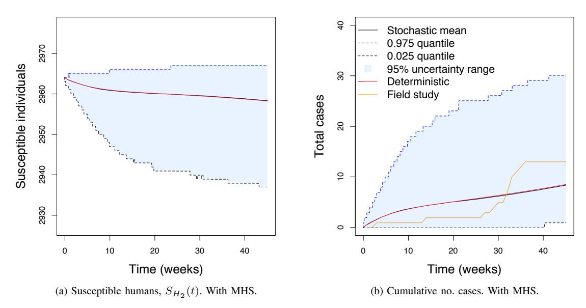
Figure 2: Average stochastic results from 1,000 independent simulations of a 44 week period, when the MHS is present. Here P = 0.1 and P ∗ = 0.5889. Plots show the mean stochastic value at each time step, along with corresponding 95% uncertainty range and quantiles, deterministic results and real world data from the 2014 MHS trial.
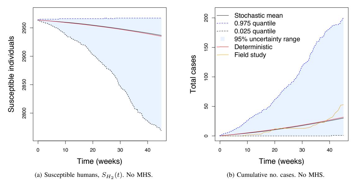
Figure 3: Average stochastic results from 1,000 independent simulations of a 44 week period, when no MHSs are present. Here P = 0.1 and P ∗ = 0. Plots show the mean stochastic value at each time step, along with corresponding 95% uncertainty range and quantiles, deterministic results and real world data from 2013.
also clearly visualise the effect of deploying the MHS within the flats. The uncertainty ranges in Figure 3, when no MHSs are used, are all much wider than the corresponding ranges found in Figure 2. For example, Figure 2b, shows we can be 95% certain that the total number of cases within the trial period will be less than 30 when the MHS is present, whereas, from Figure 3b, when no MHS is present, the upper limit on the same 95% uncertainty range shows there is potential for up to 200 new cases in the same 44 week period. Thus the MHS can greatly reduce the potential for a large numbers of infections.
The stochastic results in Figures 2b and 3b, both under-predict the final total number of cases observed within the 44 week period, compared to the real-world data. There are a variety of possible reasons for this. It could be due to random fluctuation, or it could be due to inaccurately estimating one of the parameters in the model. For example, we have chosen a daily mosquito biting rate of \(0.2 \, \mathrm{day}^{-1}\), whilst the literature generally references this value to be anywhere between \(0-3 \, \mathrm{day}^{-1}\).
Combined with the additional verification results presented in Appendix 1, these provide quantitative evidence that the new hybrid deterministic-stochastic model is functioning correctly, and accurately evolving the dengue dynamics within the flats. In the next section, we move on to demonstrate some of the unique insights that the new stochastic approach can provide, as well as demonstrating its main advantages over the deterministic equivalent.
5. SIMULATIONS AND RESULTS: STOCHASTIC INSIGHTS INTO THE MHS
5.1. Example 1: Extended deployment and distribution of possible outcomes
The hybrid deterministic-stochastic model is first used to simulate deploying the MHSs within the trial site for an extended three year period. Initial conditions are set to the same as those outlined in (14) and plots illustrating a single simulation of the three year period are shown in Figures 4 and 5. Figures 4 and 5, show a single simulation for the flats and the Kuala Lumpur populations, respectively. The number of humans infected within the flats is noticeably larger than the corresponding number of infected mosquitoes within the flats. This is expected, and shows that the model accurately captures the fact that people may become infected whilst away from the flats, in wider Kuala Lumpur. Comparing Figure 4e and Figure 4f, it is evident that the model captures the fact that not all mosquitoes survive the latent period, with the cumulative total number of infected mosquitoes over the three year period being less than the culmulative total number of latent ones. Figure 4b shows roughly 30 new cases of dengue over the three year period and an annual average of 10 new cases, which is in good agreement with the 13 cases observed during the 44 weeks of the 2014 MHS system trial. The results of the corresponding deterministic part of the model for the wider population in Kuala Lumpur are shown in Figure 5. These are of course identical to those presented in Greenhalgh et al. [17].
Total extinction of dengue within the flats is never observed in the stochastic model. This is because dengue is endemic in Malaysia's broader population. Even if no dengue infections occur within the flats, there will always be cases of residents being infected whilst in wider Malaysia and reintroducing dengue to mosquitoes in the flats when they return home. This is evident in Figure 4b and 4f, where newly infected humans are observed, despite no infectious mosquitoes being present at the same time.
The stochastic approach allows us to investigate the distribution of all potential outcomes for the simulations presented above, both with and without the MHS traps. Subsequently, the frequency distribution of the potential total number of humans infected annually within the flats is presented in Figure 6, for each of the three years. These distributions, and the figures below, have been calculated using 1,000 independent simulations. It is noted that the x-axis range on the distributions in Figure 6 has been cropped to allow for easy comparison of the results, and subsequently some higher, outlier, values as well as larger summary statistics are not visible. Corresponding summary statistics are displayed in the plot legends, and show the deterministic result for the total number of cases, alongside the stochastic mean and 95% uncertainty range from \(Q_{.025}\) to \(Q_{.975}\).
The MHS traps significantly reduce the potential for a large number of infections. When the traps are present, a significant decrease in the mean number of new cases each year is observed, along with a narrowing of the 95% uncertainty range (95% UR: \(Q_{.025}\), \(Q_{.975}\)). When the MHS is present, this mean number of new cases is 9.34 (95% UR: 1,30) in the first year, 13.78 (95% UR: 4,36.03) in the second and 20.30 (95% UR: 7,47.03) in the third. On the other hand, when no MHSs are present, the mean number of new cases increases significantly to 35.35 (95% UR: 1,234.03) in the first year, 65.30 (95% UR: 1,327.13) in the second and 1.35% UR: 1.35% UR: 1.35% UR: 1.35% UR: 1.35% UR: 1.35% UR: 1.35% UR: 1.35% UR: 1.35% UR: 1.35% UR: 1.35% UR: 1.35% UR: 1.35% UR: 1.35% UR: 1.35% UR: 1.35% UR: 1.35% UR: 1.35% UR: 1.35% UR: 1.35% UR: 1.35% UR: 1.35% UR: 1.35% UR: 1.35% UR: 1.35% UR: 1.35% UR: 1.35% UR: 1.35% UR: 1.35% UR: 1.35% UR: 1.35% UR: 1.35% UR: 1.35% UR: 1.35% UR: 1.35% UR: 1.35% UR: 1.35% UR: 1.35% UR: 1.35% UR: 1.35% UR: 1.35% UR: 1.35% UR: 1.35% UR: 1.35% UR: 1.35% UR: 1.35% UR: 1.35% UR: 1.35% UR: 1.35% UR: 1.35% UR: 1.35% UR: 1.35% UR: 1.35% UR: 1.35% UR: 1.35% UR: 1.35% UR: 1.35% UR: 1.35% UR: 1.35% UR: 1.35% UR: 1.35% UR: 1.35% UR: 1.35% UR: 1.35% UR: 1.35% UR: 1.35% UR: 1.35% UR: 1.35% UR: 1.35% UR: 1.35% UR: 1.35% UR: 1.35% UR: 1.35% UR: 1.35% UR: 1.35% UR: 1.35% UR: 1.35% UR: 1.35% UR: 1.35% UR: 1.35% UR: 1.35% UR: 1.35% UR: 1.35% UR: 1.35% UR: 1.35% UR: 1.35% UR: 1.35% UR: 1.35% UR: 1.35% UR: 1.35% UR: 1.35% UR: 1.35% UR: 1.35% UR: 1.35% UR: 1.35% UR: 1.35% UR: 1.35% UR: 1.35% UR: 1.35% UR: 1.35% UR: 1.35% UR: 1.35% UR: 1.35% UR: 1.35% UR: 1.35% UR: 1.35% UR: 1.35% UR: 1.35% UR: 1.35% UR: 1.35% UR: 1.35% UR: 1.35% UR: 1.35% UR: 1.35% UR: 1.
5.2. Example 2: Endemic equilibrium
Endemic equilibrium occurs when a disease has established itself within a population at a level that will remain constant for all time, in the absence of any intervention or other exogenous changes (e.g. to the environment) [47]. Thus, the number of infected, susceptible and recovered individuals within a population, at endemic equilibrium, gives insight into the long term impact of a disease on a population.
In this example, we calculate the endemic equilibrium values within the flats in the absence of the MHSs \((P^* = 0)\) and compare these to those predicted once MHSs have been introduced \((P^* = 0.5889)\). Results
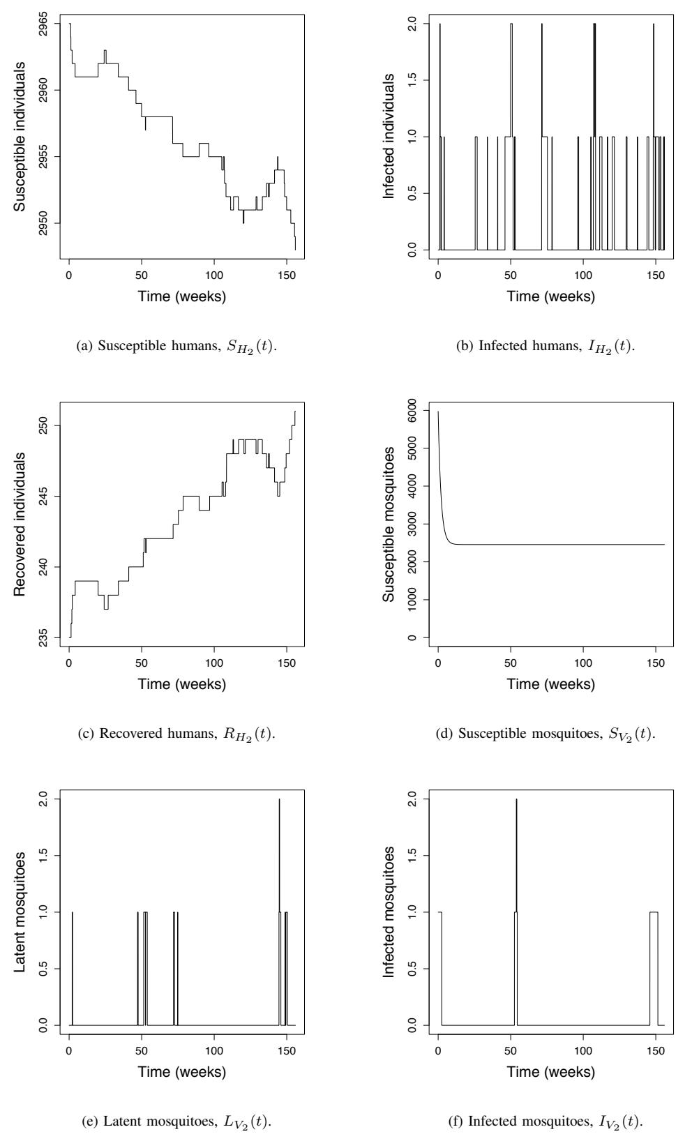
Figure 4: Stochastic simulation of the mosquito and human populations within the flats, over a three year period. Here, P = 0.1 and P ∗ = 0.5889.
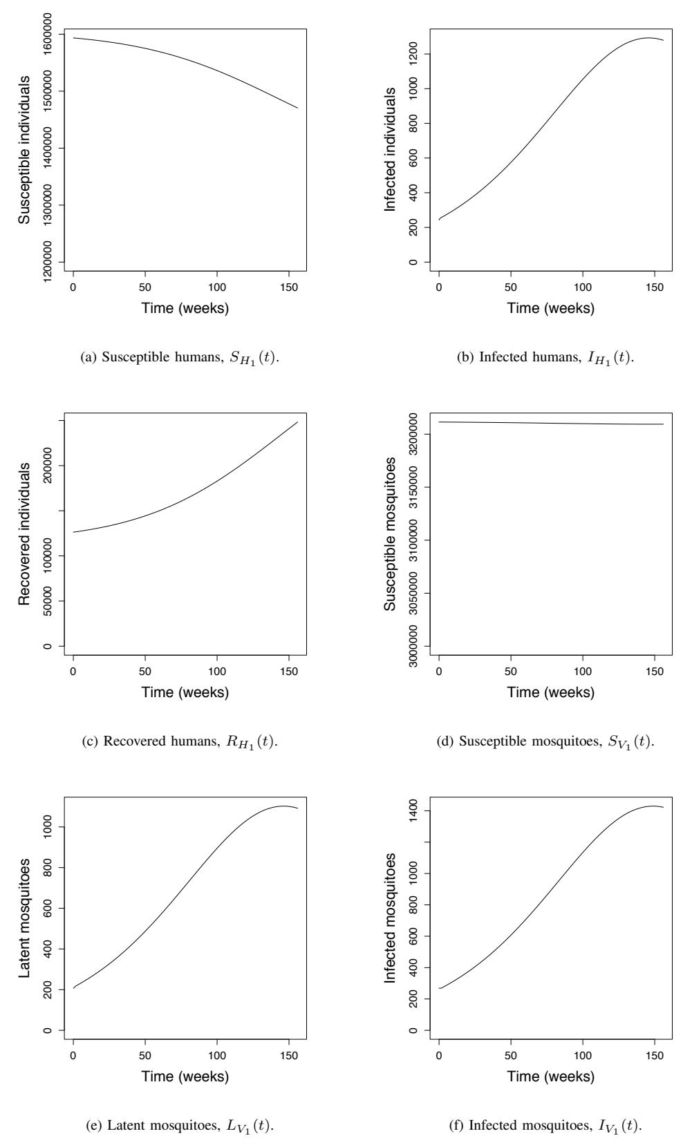
Figure 5: Results from the solution of the deterministic model for the mosquito and human populations in Kuala Lumpur, for a three year period with P = 0.1 and P ∗ = 0.5889. This part of the model is identical to that used by Greenhalgh et al. [17].
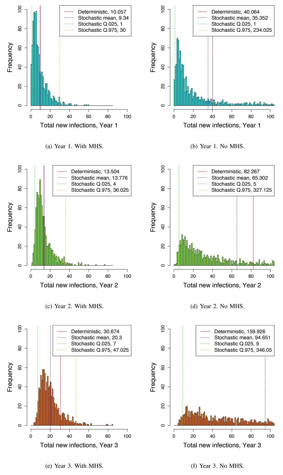
Figure 6: Frequency distribution of the total number of infected humans in the flats, per year, for each of the three years. These frequencies were calculated using the results of 1,000 independent stochastic simulations, both with the MHS, where P=0.1 and \(P^*=0.5889\) and without the MHS, where P=0.1 and \(P^*=0.5889\) and without the MHS, where P=0.1 and \(P^*=0.5889\) and without the MHS, where P=0.1 and \(P^*=0.5889\) and without the MHS, where P=0.5889 and without the MHS, where P=0.5889 and without the MHS, where P=0.5889 and without the MHS, where P=0.5889 and without the MHS, where P=0.5889 and without the MHS, where P=0.5889 and \(P^*=0.5889\) and without the MHS, where P=0.5889 and \(P^*=0.5889\) and \(P^*=0.5889\) and \(P^*=0.5889\) and \(P^*=0.5889\) and \(P^*=0.5889\) and \(P^*=0.5889\) and \(P^*=0.5889\) and \(P^*=0.5889\) and \(P^*=0.5889\) and \(P^*=0.5889\) and \(P^*=0.5889\) and \(P^*=0.5889\) and \(P^*=0.5889\) and \(P^*=0.5889\) and \(P^*=0.5889\) and \(P^*=0.5889\) and \(P^*=0.5889\) and \(P^*=0.5889\) and \(P^*=0.5889\) and \(P^*=0.5889\) and \(P^*=0.5889\) and \(P^*=0.5889\) and \(P^*=0.5889\) and \(P^*=0.5889\) and \(P^*=0.5889\) and \(P^*=0.5889\) and \(P^*=0.5889\) and \(P^*=0.5889\) and \(P^*=0.5889\) and \(P^*=0.5889\) and \(P^*=0.5889\) and \(P^*=0.5889\) and \(P^*=0.5889\) and \(P^*=0.5889\) and \(P^*=0.5889\) and \(P^*=0.5889\) and \(P^*=0.5889\) and \(P^*=0.5889\) and \(P^*=0.5889\) and \(P^*=0.5889\) and \(P^*=0.5889\) and \(P^*=0.5889\) and \(P^*=0.5889\) and \(P^*=0.5889\) and \(P^*=0.5889\) and \(P^*=0.5889\) and \(P^*=0.5889\) and \(P^*=0.5889\) and \(P^*=0.5889\) and \(P^*=0.5889\) and \(P^*=0.5889\) and \(P^*=0.5889\) and \(P^*=0.5889\) and \(P^*=0.5889\) and \(P^*=0.5889\) and \(P^*=0.5889\) and \(P^*=0.5889\) and \(P^*=0.5889\) and \(P^*=0.5889\) and \(P^*=0.5889\) and \(P^*=0.5889\) and \(P^*=0.5889\) and \(P^*=0.5889\) and \(P^*=0.5889\) and \(P^*=0.5889\) and \(P^*=0.5889\) and \(P^*=0.5889\) and \(P^*=0.5889\) and \(P^*=0.5889\) and \(P^*=0.5889\) and \(P^*=0.5899\) and \(P^*=0.5889\) and \(P^*=0.5889\) and \(P^*=0.5889\) and \(P^*=0.5889\) and \(P^*=0.5889\) and \(P^*=0.5889\) and \(P^*=0.5889\) and P
are compared to endemic equilibrium values from the deterministic model presented in Greenhalgh et al. [17], since the long-term, stochastic averages should tend towards the deterministic endemic equilibrium values, provided the stochastic results are averaged over a large enough time period.
To simulate the endemic equilibrium for the flats, in the absence of the MHS traps, the deterministic endemic equilibrium values (Table 2 in Greenhalgh et al. [17]) were used as the initial conditions. Starting at these values greatly reduces the computational time required to reach endemic equilibrium, as the stochastic model is significantly more computationally intensive than its deterministic counterpart. For this case, where P=0.1 and \(P^*=0\), these initial conditions were:
\[S_{H_1}(0) = 1,593,441,\] \(S_{V_1}(0) = 3,211,447,\) \(S_{H_2}(0) = 2,753.155,\) \(S_{V_2}(0) = 5,975.446,\) \(I_{H_1}(0) = 242,\) \(L_{V_1}(0) = 207,\) \(I_{H_2}(0) = 0.115,\) \(L_{V_2}(0) = 0.098,\) \(R_{H_1}(0) = 126,316,\) \(I_{V_1}(0) = 268,\) \(R_{H_2}(0) = 446.730,\) \(I_{V_2}(0) = 0.127.\) (15)
Similarly, for the case where the MHS traps were introduced to the flats, with P = 0.1 and \(P^* = 0.5889\), the initial conditions were taken to be:
\[S_{H_1}(0) = 1,593,441,\] \(S_{V_1}(0) = 3,211,447,\) \(S_{H_2}(0) = 3,113.127,\) \(S_{V_2}(0) = 2,456.580,\) \(I_{H_1}(0) = 242,\) \(L_{V_1}(0) = 207,\) \(I_{H_2}(0) = 0.022,\) \(L_{V_2}(0) = 0.008,\) \(R_{H_1}(0) = 126,316,\) \(I_{V_1}(0) = 268,\) \(R_{H_2}(0) = 86.850,\) \(I_{V_2}(0) = 0.010.\) (16)
Because in the stochastic model all of the variables need to be whole numbers, the initial numbers of infected and removed humans in the flats, and the initial numbers of latent and infected mosquitoes in the flats, were rounded to the nearest whole number, and the initial numbers of susceptible humans and mosquitoes in the flats adjusted accordingly. To allow endemic equilibrium to be established, the model was used to simulate an arbitrary 2,400 year period, starting in 2013. The average value of the stochastic results was then calculated over the final 1,000 years. The endemic equilibrium values are presented in Table 3. Here, the results from the deterministic model in Greenhalgh et al. [17] are again presented alongside the stochastic results to allow for easy comparison.
Table 3: Endemic equilibrium values for the new stochastic model, presented alongside those obtained using the existing deterministic model. Here, P=0.1 for all simulations.
| \(P^* = 0\) | \(P^* = 0.5889\) | |||
|---|---|---|---|---|
| Endemic Equilibrium Value | Stochastic | Deterministic | Stochastic | Deterministic |
| \(S_{H_2}(t)\) | 2,762.990 | 2,753.155 | 3,111.980 | 3,113.127 |
| \(I_{H_2}(t)\) | 0.117 | 0.115 | 0.023 | 0.022 |
| \(R_{H_2}(t)\) | 436.89 | 446.73 | 88.00 | 86.85 |
| \(S_{V_2}(t)\) | 5,976.22 | 5,975.44 | 2,456.57 | 2,456.58 |
| \(L_{V_2}(t)\) | 0.102 | 0.098 | 0.016 | 0.008 |
| \(I_{V_2}(t)\) | 0.128 | 0.127 | 0.010 | 0.010 |
| Incidence Cases (Per week) | 0.115 | 0.115 | 0.022 | 0.022 |
| Total Cases (Per year) | 5.99 | 5.96 | 1.146 | 1.158 |
The results in Table 3 firmly support the conclusion that the stochastic model is functioning as desired, and accurately simulating the evolution of the human and mosquito populations within the flats. It is also noted, that the implementation of the MHS clearly reduces both the number of infected people and latent and infected mosquitoes present at endemic equilibrium. This is accompanied by an increase in the number of susceptible individuals and a decrease in the number of recovered individuals when the MHS is present, implying that fewer people have contracted the disease as a direct result of the MHS.
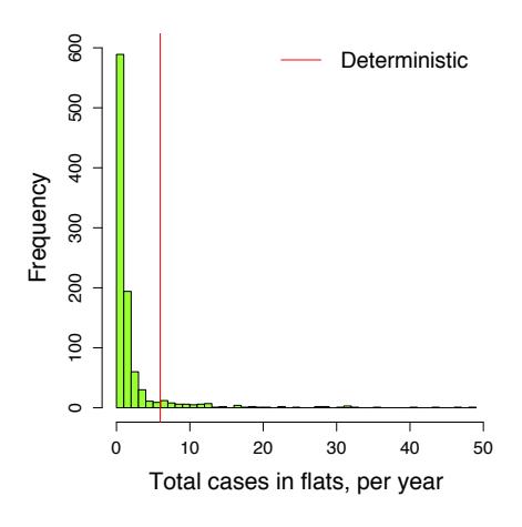
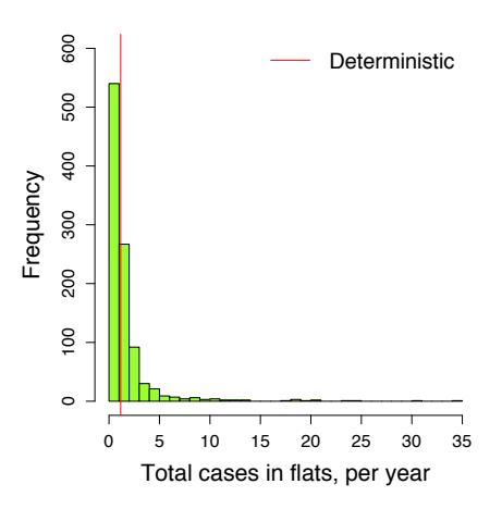
The new model can also calculate the distribution of possible outcomes at endemic equilibrium in two ways: The first technique, Method I, uses a single stochastic simulation of 1,500 years, and records the annual number of dengue cases for every year. Combined, these give the distribution of possible outcomes pictured in Figure 7. The second technique, Method II, can be found in Appendix 2 and uses a series of 1,000 independent simulations of a three year period, starting at the deterministic endemic equilibrium values outlined in (15) and (16), to produce the equivalent distribution. For each method, results are obtained both with and without the MHS traps, using \(P^* = 0\) and \(P^* = 0.5889\), respectively.
The results produced by Method I (Figure 7) show the distribution of the total number of dengue infections expected annually, both with and without MHS intervention in the flats. The frequency distributions, the means and the modal frequencies are calculated using the final 1,000 years.
(a) Distribution of possible outcomes at endemic equilibrium, \(P^*=0\).
(b) Stochastic \(S_{H_2}(t)\), plotted against deterministic endemic equilibrium \(P^{*}=0\).
(c) Distribution of possible outcomes at endemic equilibrium, \(P^{*}=0.5889.\)
(d) Stochastic \(S_{H_2}(t)\), plotted against deterministic endemic equilibrium , \(P^*=0.5889\).
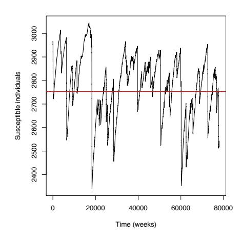
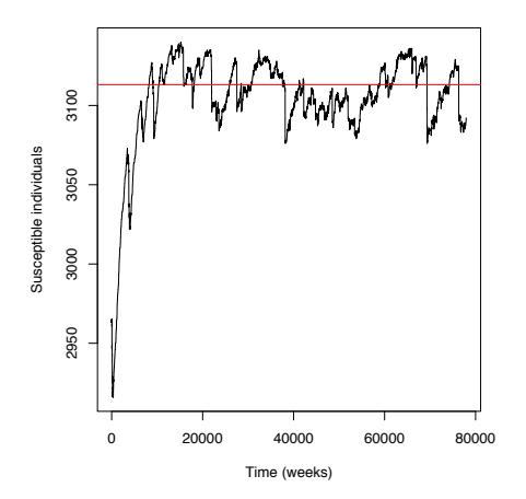
Figure 7: Distribution of possible outcomes at endemic equilibrium, calculated using Method I. Plots (a) and (c) show the results for \(P^*=0\) and \(P^*=0.5889\), respectively. Plots of the average susceptible humans in the flats over each separate year are found in (b) and (d), with the corresponding deterministic endemic equilibrium value plotted in red.
It is observed that when the MHS is present, the range of potential new dengue cases at endemic equilibrium is much narrower than the case where no MHS is used. This is evident from the maximum value of the distribution of just 35 dengue cases annually with the MHS present, compared to a potential for up to 335 cases without it. It is noted that the x-axis range in Figure 7a has been cropped to allow ease of legibility, so these higher, outlier values are not visible. The modal frequency, both with and without the MHS, is zero cases annually within the flats. However, the mean annual number of cases when no MHS is present is 5.50 (95% UR: 0, 52.15), which is noticeably bigger than the corresponding value of 1.17 (95% UR: 0, 8) when the mosquito traps are deployed, and so we can again safely conclude that the MHS has a significant impact on reducing the potential for new dengue cases within the flats.
Plots of the number of susceptible humans within the flats have also been included here, in Figure 7b and 7d. These show the variations in the number of susceptible humans within the trial site over the entire 1,000 year period, and are included to illustrate the way in which the stochastic predictions oscillate around the deterministic endemic equilibrium values, indicated by the red line.
5.3. Effect on Malaysian chemical fogging activities
In Malaysia, by law, health care practitioners must report new dengue cases to the Malaysian Ministry of Health within 24 hours of discovery. This triggers a chain of events that results in chemical fogging with insecticide sprays in the area surrounding every newly reported case. In 2010, within the Klang Valley district where the flats are located, the cost of chemical fogging was estimated to be 811 USD per reported case [6]. On average, 61% of these costs were for human resources, whilst 14% of the costs were for the chemical insecticides, and the remainder covered fogging equipment and vehicles.
In comparison, each MHS unit costs 2 USD, requires 18 USD worth of solution annually, and incurs maintenance costs of 24 USD per year. These figures are obviously subject to change, and increased production of the MHS will reduce costs further. Based on these figures, the 552 MHSs used in the 44 week trial would incur an initial set-up cost of 1,104 USD to buy MHSs, and running costs would total 19,617 USD for the 44 week period. In contrast, we expect 35 cases on average for the same period, when no MHSs are present, which would result in 28,385 USD worth of chemical fogging expenses. This translates to a 30% reduction in the cost of dengue control activities when MHSs are used within the Ridzuan Court flats if the start up MHS costs are spread over three years. If the MHSs were to be rolled out across the Klang Valley, the total savings of the district are only expected to increase further.
6. CONCLUSION
A novel set of hybrid deterministic-stochastic equations has been outlined, and successfully used to model the spread of dengue amongst the human and mosquito population within three blocks of highrise flats in the Klang Valley in Malaysia. The unique model truly captures the random nature of the dengue dynamics within the flats. One main benefit of this approach is its ability to capture uncertainty and variability, which are both of high importance to decision makers across the globe. This makes the model a powerful tool for epidemic modellers and disease control specialists worldwide, as it allows for quick and easy visualisation of all possible scenarios when designing control strategies to suppress the spread of the virus. This is something that will be of key importance when the model is later rolled out into the publicly available app that is being designed to complement the MHS traps.
A single stochastic simulation of the flats is also more intuitive to interpret, since only whole numbers of people or mosquitoes can become infected at any one time. On the other hand, in the deterministic approach, it is commonplace to have fractions of a mosquito infected, or a fraction of a human dying. Further, the stochastic model may be used to simulate the distribution of all possible outcomes.
The MHS traps clearly produce a large reduction in the mean number of dengue cases observed annually. This is accompanied by a significant narrowing of the corresponding uncertainty range. For the 44 week MHS trial, the mean total number of cases decreased from 35 with no MHSs, to just 9 cases when MHSs were introduced. The corresponding 95% uncertainty range also narrowed from (1, 234) without the MHSs, to (1, 30) when the MHSs were introduced. A significant reduction in the annual number of dengue cases at endemic equilibrium is also observed, which can be directly linked to the introduction of the MHS traps. This figure decreases from 5.99 cases annually, when no MHSs are present, to just 1.146 cases when the MHS is introduced (see Table 3). This clearly implies that the MHS traps produce a sustainable reduction in both the dengue-infected mosquito population, as well as the number of human dengue cases observed within the local community.
The findings above have been echoed by other studies into the use of mosquito traps to combat vectorborne diseases. Sharp et al. [48] demonstrate that the presence of autocidal gravid ovitraps (AGOs) is strongly linked to a significant reduction in Chikungunya virus cases in Puerto Rico. The AGO traps attract, capture and kill ovipositing female mosquitoes using a sticky lining, rather than an insecticide. With AGO traps present, Sharp et al. estimate that only 10.3% of local residents will contract the Chikungunya virus, in contrast to 48.7% with no traps. This further supports the downward trend in dengue cases that is observed when the MHS traps are present.
Whilst the hybrid stochastic-deterministic model simulates a more realistic picture of the random events within nature that spread the dengue virus, it does have a few minor limitations. It is slightly more computer intensive than the purely deterministic approach, however the time step ∆t can be chosen to minimise this increase, whilst maintaining the accuracy of predictions. The model also does not account for seasonality or climate-forced changes, and the fluctuation in the number of mosquitoes that this usually causes. However, as it is, it provides a very simple and easy to use tool to give a quick, accurate approximation of the dengue dynamics within the flats.
This paper has focused on the application of the hybrid deterministic-stochastic model to three specific blocks of flats, however this model could easily be modified and implemented anywhere in the world, to simulate the effect of any auto-dissemination type mosquito trap. It can quickly and easily be used to predict the impact of deploying the mosquito traps within similar environments, making it extremely useful when planning mosquito control activities. In the right hands, it has potential to be a very useful and easy to use tool in the fight against dengue.
ACKNOWLEDGEMENTS
This work was funded through the British Council in Malaysia, as part of their Dengue Tech Challenge (Application reference: DTC 16022), under the Newton-Ungku Omar Fund partnership, the Scottish Funding Council's Global Challenges Research Fund (GCRF), alongside EPSRC and the University of Strathclyde, UK, who provided funding from the 2016 EPSRC Global Challenges Research Fund, Institutional Award (EPSRC reference: EP/P511055/1). The Dengue Tech Challenge grant was funded by the UK Department for Business, Energy and Industrial Strategy and the Malaysian Industry-Government Group for High Technology (MIGHT) and delivered by the British Council and PlaTCOM ventures. The authors are grateful to One Team Networks Sdn Bhd, in Malaysia, as our principal collaborator in Malaysia for the Dengue Tech Challenge 2016 and for providing the data.