

1. INTRODUCTION
The most recent factsheets of the World Health Organization state that about 17.9 million people died of cardiovascular diseases in 2019, which accounts for 32% of all global deaths [1]. Among these, atherosclerotic heart disease (ASCVD) remains a leading cause of death worldwide despite significant advances in diagnosis and treatment procedures. It is a chronic inflammatory disease of the large and medium-sized arteries, which is often responsible for death. In various animal and patient models, it is observed that cardiopalmus or heart beat is also directly associated with coronary atherosclerosis. It has also been confirmed in several studies that if the heart beat is increased then in most cases it is due to the increased progression of coronary atherosclerosis, while lower heart beat is connected with decreased cardiovascular and complications [2], [3]. In these patients, the chances of plaque rupture are very high. Additionally, inflammation contributes significantly to the pathogenesis and progression of atherosclerosis, which makes the disease more severe. In the literature, many researchers considered various risk factors of atherosclerosis disease, such as a rich fatty diet, type-2 diabetes, and many more.
In various treatments, the reduction of atherosclerosis by combining anti-inflammation and inhibitiondegradation of the plaque is discussed [4]. In the last decade, Sacks et al. [5] have studied saturated fatty acids (SFAs) in rich diets given to humans and found this to be an important factor directly linked to an increase in atherosclerosis. After three years in an experiment on mice, Lian et al. [6] replaced this SFA with other SFA, namely polyunsaturated fatty acids, and observed that it could reduce atherosclerosis. As we
∗Corresponding author
Received March 17th, 2023, Revised June 8th, 2023 (first), Revised July 6th, 2023 (second), Accepted for publication August 21st , 2023. Copyright ©2023 Published by Indonesian Biomathematical Society, e-ISSN: 2549-2896, DOI:10.5614/cbms.2023.6.2.3
know, statins are a class of drugs used to control atherosclerosis. Basically, it targets HMG-CoA reductase, which acts as an enzyme in the rate-limiting step of cholesterol biosynthesis [7]. Moghaddam et al. found that patients with type-2 diabetes are more likely to develop atherosclerosis which can subsequently lead to dementia through various pathways [8].
Various clinical studies have shown that oxidative transformation of LDL plays an important role in the genesis of atherosclerosis. It begins when LDL is modified through endothelial cells during the oxidation process and is rapidly deposited by macrophages, which are the major contributors to foam cell formation [9], [10], [11], [12]. In 1984, Heineke et al. [13] found that any alteration of LDL during incubation with arterial smooth muscle cells was affected and supported by increasing Fe and Cu concentration, whereas no effect of Zn was found. In the previous study, Henriksen et al. [12] have shown that LDL customized by incubation through endothelial cells or guinea pig arterial smooth muscle cells is more speedily destroyed by macrophages compared to native LDL. LDL modified by incubation with human smooth muscle cells that are incorporated by human monocyte-derived macrophages and resident mouse peritoneal macrophages into larger amounts of cholesterol esters than control LDL.
Cytokines are low-molecular-weight protein intermediaries that more often than not act at small choice between neighboring cells in lymphoid organs or reddened tissues. Cytokines are produced by all kinds of cells implicated in atherosclerosis, which act on different targets applying multiple effects and are mostly responsible for the interaction between endothelial, leucocytes, smooth muscle cells, and other vascular living cells. These cytokines are classified as pro- and anti-atherogenic cytokines, which are two separate groups depending on whether they stimulate or inhibit atherogenesis. The main pro-atherogenic cytokines viz. tumor necrosis factor−α, interleukin−1a, and 17 are secreted by macrophages, lymphocytes, natural killer cells, and vascular smooth muscle cells, while anti-atherogenic cytokines identified as transforming growth factor−β (TGF−β), interleukin-10 and 35 [14], [15]. Recently, Hafien and Dascalopoulou [16] have discussed studies on canakinumab anti-inflammatory thrombosis outcomes as well as therapeutic agents to specify the inflammatory pathway in atherosclerotic heart disease and demonstrated the effects of various antiinflammatory agents in patients with ASCVD. In several experimental results, researchers found that proand anti-cytokine profile extensively differs between patients with high and low coronary plaque volume. Certain cytokines such as IL − 1a and IL − 17 play a major pro-atherogenic role in vulnerable plaque formation, while MCP-1 cytokine shows paradoxically protective effects [17], [18]. However, in experiments, some researchers observed that different cytokines behave in both natures and whose effects cannot be left forever.
The aim of this study is to express the measures and effects of pro- and anti-inflammatory cytokines with the help of a system of reaction diffusion equation model and to demonstrate an auxiliary approach to their future prediction. The present study is arranged in the following order. The mathematical description of the chronic inflammatory response with the inclusion of biochemical and mechanical parameters is presented in Section 2. In the next Section 3, we express the proposed model in the form of reaction dynamical system and discuss the existence of the solutions, and determine the equilibrium points for the model. Local and global stability analysis of this model is shown in Section 4. Subsequently, we further discuss the numerical results and discussion for the model in Section 5. Finally, we conclude all the results and outcomes in Section 6.
2. MODEL DESCRIPTION
The present study investigates the chronic inflammatory response of atherosclerosis as well as its biochemical and mechanical behaviour. We presented a mathematical model based on several assumptions and taking into account three main compartments namely, immune cells (M), pro-cytokines (P), and anticytokines (A), which is shown in Figure 1. This is formulated by a reaction-diffusion system in onedimensional space with the concentration of immune cells (macrophage, monocytes) and two types of responsible inflammatory cytokines, viz. pro-inflammatory cytokines(IL − 1, TNF−α, IL − 12) [19], [20], and anti-inflammatory cytokines(IL − 10, IL − 6, TGF−β) [4], [16], [21]. These two cytokines are secreted by immune cells. In accordance with the inflammatory nature of pro-inflammatory cytokines, these cytokines are specifically responsible for making atherosclerosis worse, while anti-inflammatory cytokines are known to reduce inflammation [14]. To formulate the mathematical problem, we assume that all compartments are diffusing with appropriate diffusion coefficients, here, x is considered between 0 and finite length L.
Table 1: Description of variables and parameters of the model.
| Variables / Parameters | Description |
|---|---|
| M | Concentration of immune cells (macrophage, monocytes) |
| P | Concentration of pro-inflammatory cytokines |
| A | Concentration of anti-inflammatory cytokines |
| α1 | Initial recruitment of immune cells due to presence of ox-LDLs |
| α2 | Secretion rate of pro-inflammatory cytokines by itself |
| α3 | Secretion rate of anti-inflammatory cytokines by inflammatory macrophages. |
| β1 | Activation rate of macrophages promoted by pro-inflammatory cytokines |
| β2 | Reduction rate of macrophages due to the presence of anti-inflammatory cytokines |
| λ1 | death rate of immune cells |
| λ2 | decay rate of pro-inflammatory cytokines |
| λ3 | decay rate of anti-inflammatory cytokines |
| τ1 | Mechanical saturation time |
| τ2 | Time taken to inhibit pro-inflammatory cytokines by anti-inflammatory cytokines |
| δ | Portion of secreted anti-inflammatory cytokines behaving like pro-inflammatory cytokines |
| d1 | diffusion coefficient of immune cells |
| d2 | diffusion coefficient of pro-inflammatory cytokines |
| d3 | diffusion coefficient of anti-inflammatory cytokines |
Figure 1: Schematic diagram of Atherosclerosis formation.
2.1. Equation for Immune Cells (M)
The evolution of the immune cells into the intima is defined as
\[\frac{\partial M}{\partial t} = d_1 \frac{\partial^2 M}{\partial x^2} + \frac{\alpha_1 + \beta_1 P - \beta_2 A}{1 + \frac{(P + A)}{\tau_1}} - \lambda_1 M. \tag{1}\]
Here, the first term on the right-hand side describes the diffusion of immune cells. The second term is considered as a Beddington-DeAngelis type of functional response [22], [23] which is used for competitive exclusion and coexistence in this model that also involves mutual interference of both immune cells and cytokines. The third term stands for the degradation of Immune cells. The functional response in the second term is considered through the following factors:
- 1) α1 corresponds to the initial recruitment of immune cells due to the existence of unnecessary ox-LDLs [14], [24].
- 2) β1P represents the evolution of immune cells promoted by pro-inflammatory cytokines [14], [25].
- 3) The term β2A opposes the secretion of immune cells due to the presence of anti-inflammatory cytokines [24], [26].
- 4) 1 + (P + A)/τ1 is the mechanical saturation factor of the immune cells, where τ1 is the time taken for the saturation [25].
Figure 2: Compartmental flow-chart diagram of the model.
2.2. Equation for Pro-inflammatory Cytokines (P)
The formation of pro-inflammatory cytokines is represented by the following reaction-diffusion equation,
\[\frac{\partial P}{\partial t} = d_2 \frac{\partial^2 P}{\partial x^2} + \frac{\alpha_2 PM}{1 + \frac{A}{\tau_2}} + \delta \alpha_3 AM - \lambda_2 P. \tag{2}\]
Here, α2 is the secretion rate of pro-inflammatory cytokines by itself, 1 + A/τ2 represents the inhibition effect of pro-inflammatory cytokines due to the presence of anti-inflammatory cytokines, τ2 is the inhibition time to act [14], α3 is the secretion rate of anti-inflammatory cytokines from immune cells, δ is the ratio of secreted anti-inflammatory cytokines behaving like pro-inflammatory cytokines (TGF-beta, IL-6) [27], [28]. In several studies, IL-6 shows both anti and pro–inflammatory effects during inflammation of atherosclerosis [27], [28].
2.3. Equation for Anti-inflammatory Cytokines (A)
The formation of anti-inflammatory cytokines satisfies the following equation
\[\frac{\partial A}{\partial t} = d_3 \frac{\partial^2 A}{\partial x^2} + (1 - \delta) \alpha_3 A M - \lambda_3 A. \tag{3}\]
In general, macrophages are mainly responsible for secretion of cytokines. Here, we consider \(\alpha_3\) is the formation rate of anti-inflammatory cytokines from immune cells. In the equations (1)-(3), terms \(d_1 \frac{\partial^2 M}{\partial x^2}\), \(d_2 \frac{\partial^2 P}{\partial x^2}\) and \(d_3 \frac{\partial^2 A}{\partial x^2}\) represent the diffusion inside intima, and the terms \(-\lambda_1 M\), \(-\lambda_2 P\) and \(-\lambda_3 A\) represent the decaying rate of the M, P and A, respectively.
In this study, we considered the initial conditions to be a function of x [29],
\[M(0,x) = M_0(x), P(0,x) = P_0(x), A(0,x) = A_0(x),\] (4)
and the homogeneous Neumann boundary conditions,
\[M_x(t,0) = 0, P_x(t,0) = 0, A_x(t,0) = 0,\] (5)
\[M_x(t,L) = 0, P_x(t,L) = 0, A_x(t,L) = 0.\] (6)
The authors are confident that the proposed model (1)–(6) is able to provide new insights into the role of pro- and anti-cytokines in the inflammation and reduction of atherosclerosis.
3. Analysis of the Model
The analytical study of any mathematical model must be a strong and fundamental part of any biological phenomenon that must be clearly described. In this section, we describe the solution of the deterministic atherosclerosis model that always exists or exists with a particular condition. The uniqueness of the solution is also important which has been established through rigorous calculations. In the context of atherosclerosis modeling, the diffusion term refers to the transport or movement of molecules such as lipids, immune cells, and inflammatory mediators within the arterial wall, while the reaction term represents the chemical involved in atherosclerosis, such as the oxidation of lipids, inflammation, and the formation of foam cells. These reactions are essential for plaque development and can influence the stability and vulnerability of plaques [24], [29]. To determine the conditions for measuring the inflammatory response over time we first analyze only the reaction part of a model (1)–(6).
3.1. The Reaction Dynamical System
The reaction dynamical ODE system is defined as,
\[\frac{dM}{dt} = \frac{\alpha_1 + \beta_1 P - \beta_2 A}{1 + \frac{(P+A)}{\tau_1}} - \lambda_1 M,\] \[\frac{dP}{dt} = \frac{\alpha_2 PM}{1 + \frac{A}{\tau_2}} + \delta \alpha_3 AM - \lambda_2 P,\] \[\frac{dA}{dt} = (1 - \delta) \alpha_3 AM - \lambda_3 A.\] (7)
In the next subsections, we have discussed the existence and uniqueness of the solution [30], [31], and after that, we calculated all possible equilibrium points of the reaction model (7).
3.2. Existence and Uniqueness of the Solution
In this subsection, we discussed the existence of solutions to this system of equations by the analytical method [30], [31], i.e., the Lipchitz condition [32], which showed that the solution is unique under derived conditions. Now, first, we simplified the equations of (7), and we get
\[M(t) - M(0) = \int_{0}^{t} \left[ \frac{\alpha_1 + \beta_1 P(s) - \beta_2 A(s)}{1 + \frac{(P(s) + A(s))}{\tau_1}} - \lambda_1 M(s) \right] ds = \int_{0}^{t} k_1 (s, M, P, A) ds, \tag{8}\]
\[P(t) - P(0) = \int_{0}^{t} \left[ \frac{\alpha_2 P(s) M(s)}{1 + \frac{A(s)}{\tau_2}} + \delta \alpha_3 A(s) M(s) - \lambda_2 P(s) \right] ds = \int_{0}^{t} k_2 (s, M, P, A) ds, \tag{9}\]
\[A(t) - A(0) = \int_{0}^{t} \left[ (1 - \delta) \alpha_3 A(s) M(s) - \lambda_3 A(s) \right] ds = \int_{0}^{t} k_3 (s, M, P, A) ds.\] (10)
We consider the kernels, \[\text{[rumus tidak dapat ditampilkan dengan baik — lihat PDF asli]}\]
\(\delta\alpha_3 AM - \lambda_2 P\) and \(k_3\) \((t, M, P, A) = (1 - \delta)\alpha_3 AM - \lambda_3 AM\) for simplification. Next, we shall prove that \(k_1\), \(k_2\) and \(k_3\) satisfy Lipchitz's condition. Also, Consider \(||M|| = m = \sup\{M, \forall t \in \Re^+\}\) and \(||A|| = a = \inf\{A, \forall t \in \Re^+\}\). Therefore, for the first kernel \(k_1\) (t, M, P, A), if \(k_1 \leq \eta_1\),
\[||k_1(t, M, P, A) - k_1(t, M_1, P, A)|| = |\lambda_1||M_1(t) - M(t)|| \le \eta_1 ||M(t) - M_1(t)||\] (11)
Similarly, we have taken the second and third kernels, and we get
\[||k_{2}(t, M, P, A) - k_{2}(t, M, P_{1}, A)|| = ||\left(\frac{\alpha_{2}PM}{1 + \frac{A}{\tau_{2}}} + \delta\alpha_{3}AM - \lambda_{2}P\right) - \left(\frac{\alpha_{2}P_{1}M}{1 + \frac{A}{\tau_{2}}} + \delta\alpha_{3}AM - \lambda_{2}P_{1}\right)||\] \[= ||\frac{\alpha_{2}M}{1 + \frac{A}{\tau_{2}}} - \lambda_{2}|||P(t) - P_{1}(t)||\] \[\leq \eta_{2}||P(t) - P_{1}(t)||, \qquad if \quad ||\frac{\alpha_{2}m}{1 + a/\tau_{2}} - \lambda_{2}|| \leq \eta_{2}.\] \[(12)\]
Finally, we check Lipchitz's condition for the third kernel \(k_3\). So,
\[||k_{3}(t, M, P, A) - k_{3}(t, M, P, A_{1})|| = ||(1 - \delta) \alpha_{3}AM - \lambda_{3}A - (1 - \delta) \alpha_{3}A_{1}M - \lambda_{3}A_{1}||\] \[= ||(1 - \delta) \alpha_{3}M - \lambda_{3}|||A(t) - A_{1}(t)||\] \[\leq \eta_{3}||A(t) - A_{1}(t)||, \quad if \quad ||(1 - \delta) \alpha_{3}M - \lambda_{3}|| \leq \eta_{3}.\] \[(13)\]
Thus, we say that all the kernel functions satisfy Lipchitz's condition for some finite value of \(\eta_1, \eta_2\) and \(\eta_3\).
Theorem 3.1. The reaction dynamical system (7) has a unique solution, iff \(\lambda_1 \leq \eta_1\), \(\|\frac{\alpha_2 m}{1 + a/\tau_2} - \lambda_2\| \leq \eta_2\), and \(\|(1 - \delta)\alpha_3 m - \lambda_3\| \leq \eta_3\) where \(\eta_1, \eta_2\) and \(\eta_3\) are some positive real numbers.
Biological Interpretation: This Theorem 3.1 clearly shows that for the above conditions, the solution of the reaction-dynamical model has either non-inflammatory or inflammatory form of the disease. Two different possibilities never occurred at the same time.
3.3. Equilibrium Points
In this section, we calculated the equilibrium points for the steady state reaction dynamical system (7), and we get the following feasible equilibrium points [30], [33].
- 1) Non-inflammatory Equilibrium Point: After doing the calculation, we can see that non-inflammatory equilibrium point or cytokines free equilibrium point \(E_0(\alpha_1/\lambda_1,0,0)\) exists without any condition, where the patient will recover from atherosclerosis without any influence of external biological affair. This shows that the patient survives without the disease if he or she follows a good routine and healthy diet.
- 2) Chronic Equilibrium Point: We also find another equilibrium point \(E_1(M_1,P_1,A_1)\), where \(M_1=\lambda_2/\alpha_2, P_1=K_1\tau_1/K_2, A_1=0\) with \(K_1=(\alpha_1\alpha_2-\lambda_1\lambda_2), K_2=(\lambda_1\lambda_2-\alpha_2\beta_1\tau_1)\), which exists where anti-inflammatory cytokines are not present in the arterial intima. This is called the chronic equilibrium point because atherosclerosis persists within the intima. The point will exist if either \(K_1>0, K_2>0\) or \(K_1<0, K_2<0\), where all parameters are positive.
- 3) Coexistence Equilibrium Point: The coexistence equilibrium point \(E^*(M^*, P^*, A^*)\) is an extremely sensitive equilibrium point in which immune cells, pro-inflammatory cytokines, and anti-inflammatory cytokines persist. Such a case occurs when atherosclerosis increases or decreases over time in relation to the existing parameters. The existence and stability analysis of this equilibrium point is further discussed with the help of Bellman and Cooke's theorem [34], [35]. All these equilibrium states are biologically valid. The stability of these equilibrium points is discussed in the next section.
4. STABILITY ANALYSIS OF EQUILIBRIUM POINTS
As we know the stability of the equilibrium points is important for any dynamical model. After obtaining the non-inflammatory, chronic, and coexistence points we will now examine the stability of the equilibrium states. In the next subsections, we discuss the local stability analysis at these equilibrium points with the help of Lyapunov's first method and the global stability analysis with the help of Bellman and Cook's theorem.
4.1. Stability Analysis of Non-inflammatory Equilibrium Point
Lyapunov's first method is used to determine the local stability at the non-inflammatory equilibrium point \((E_0)\). Initially, we define a Jacobian matrix for the system (7),
\[J(M, P, A) = \begin{pmatrix} -\lambda_1 & \frac{\beta_1}{1 + \frac{A+P}{1}} - \frac{\alpha_1 - A\beta_2 + \beta_1 P}{\tau_1 \left(1 + \frac{A+P}{\tau_1}\right)^2} & -\frac{\beta_2}{1 + \frac{A+P}{\tau_1}} - \frac{\alpha_1 - A\beta_2 + \beta_1 P}{\tau_1 \left(1 + \frac{A+P}{\tau_1}\right)^2} \\ \alpha_3 \delta A + \frac{\alpha_2 P}{1 + \frac{A}{\tau_2}} & \frac{\alpha_2 M}{1 + \frac{A}{\tau_2}} - \lambda_2 & \alpha_3 \delta M - \frac{\alpha_2 M P}{\tau_2 \left(1 + \frac{A}{\tau_2}\right)^2} \\ \alpha_3 (1 - \delta) A & 0 & \alpha_3 (1 - \delta) M - \lambda_3 \end{pmatrix}.\] (14)
Now, the Jacobian at the point \(E_0(\alpha_1/\lambda_1, 0, 0)\), becomes,
\[J(E_0) = \begin{pmatrix} -\lambda_1 & \beta_1 - \frac{\alpha_1}{\tau_1} & -\beta_2 - \frac{\alpha_1}{\tau_1} \\ 0 & \frac{\alpha_1 \alpha_2}{\lambda_1} - \lambda_2 & \frac{\alpha_1 \alpha_3 \delta}{\lambda_1} \\ 0 & 0 & \frac{\alpha_1 \alpha_3 (1 - \delta)}{\lambda_1} - \lambda_3 \end{pmatrix}.\] (15)
After defining the characteristic equation for equation (15), we get
\[(\lambda + \lambda_1)(\lambda_1(\lambda + \lambda_2) - \alpha_1\alpha_2)(\lambda_1(\lambda + \lambda_3) - \alpha_1\alpha_3(1 - \delta)) = 0, \tag{16}\] where, \(\lambda\) is the eigenvalue of the Jacobian matrix (15) at \(E_0\), which are \(-\lambda_1, (\alpha_1\alpha_2 - \lambda_1\lambda_2)/\lambda_1\) and \((\alpha_1\alpha_3 - \delta\alpha_1\alpha_3 - \lambda_1\lambda_3)/\lambda_1\). Hence, it is stable if \(\alpha_1/\lambda_1 < \lambda_2/\alpha_2\) and \(\alpha_1/\lambda_1 < \lambda_3/(\alpha_3(1-\delta))\)).
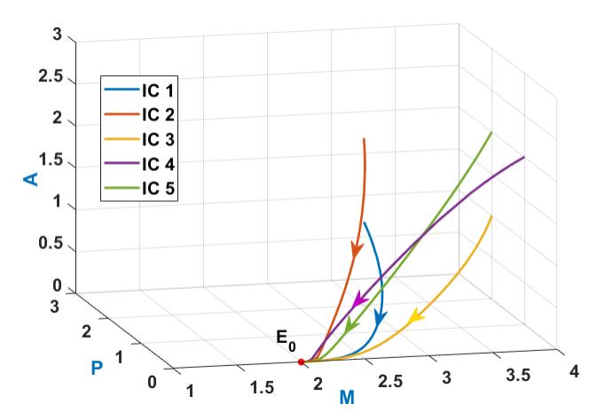
Figure 3: Stability of the non-inflammatory equilibrium pointE0 when α1/λ1 < min{λ2/α2, λ3/(α3(1 − δ))}. The trajectories are obtained from the system (7) for different initial values of M, P andA.
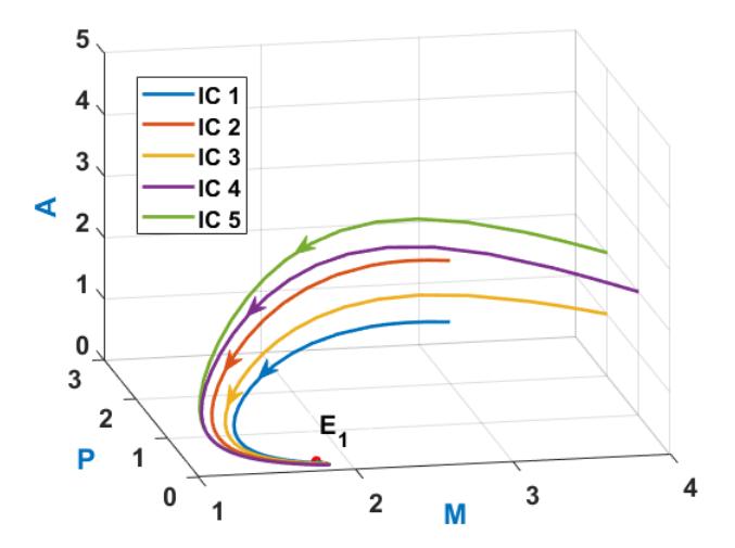
Figure 4: . Stability of the chronic equilibrium point E1 when λ1/2 > p K1K2/(K1 + K2) and λ2/α2 < λ3/(α3(1 − δ)). The trajectories are obtained from the system (7) for different initial values of M, P and A.
Theorem 4.1. The reaction dynamical system (7) always has a non-inflammatory equilibrium point E0, and it is stable if α1/λ1 < min{λ2/α2, λ3/(α3(1 − δ))}.
Biological Interpretation: The above condition in theorem 4.1 confirms that if a low ox-LDL concentration is present in the intima region compared to cytokines level, there is no chance to trigger chronic inflammation. The inflammation will definitely disappear.
4.2. Stability Analysis of Chronic Equilibrium Point
Now, we define the characteristic equation from equation (14) at chronic equilibrium point,
\[\left(\alpha_2(\lambda+\lambda_3)-\alpha_3(1-\delta)\lambda_2\right)\left(K_1^2\lambda(\lambda+\lambda_1)+K_2^2\lambda(\lambda+\lambda_1)+K_1K_2(\alpha_1\alpha_2+2\lambda(\lambda+\lambda_1)-\alpha_2\beta_1\tau_1)\right)=0,\] (17) where, \(\lambda\) is the root of the equation (17), which are \(-\frac{\lambda_1}{2}\pm\sqrt{\left(\frac{\lambda_1}{2}\right)^2-\frac{K_1K_2}{(K_1+K_2)}}\) and \(\frac{\alpha_2\lambda_3-\alpha_3(1-\delta)\lambda_2}{\alpha_2}\).
- Case I: If \(K_1 > 0, K_2 > 0\)A) When \(\frac{\lambda_1}{2} < \sqrt{\frac{K_1 K_2}{(K_1 + K_2)}}\) and \(\frac{\lambda_2}{\alpha_2} < \frac{\lambda_3}{\alpha_3 (1 \delta)}\), then one pair of eigenvalues of the equation (17) must be complex with negative real parts. Hence, the equilibrium point will be asymptotically stable.
- B) When \(\frac{\lambda_1}{2} > \sqrt{\frac{K_1 K_2}{(K_1 + K_2)}}\) and \(\frac{\lambda_2}{\alpha_2} < \frac{\lambda_3}{\alpha_3 (1 \delta)}\), then all the eigenvalues of the equation (17) must be negative. Hence, the equilibrium point will be stable.
Case – II: If \(K_1 < 0, K_2 < 0\), then at least one eigenvalues of the equation (17) must be positive. Hence, the equilibrium point will be unstable.
4.3. Stability Analysis of Coexistence Equilibrium Point
It is very tedious to examine the stability of the coexistence equilibrium point \(E^*(M^*, P^*, A^*)\) analytically. For this reason, we used Bellman and Cooke's theorem to determine global stability.
Bellman and Cooke's Theorem
Let \(\Im(z) = \mu(z, e^z)\), where \(\mu(z, e^z)\) is a polynomial with principal term. The function \(\Im(iw)\) is now separated into real and imaginary parts, i.e., we set \(\Im(iw) = \phi(w) + i\psi(w)\). If all the zeros of the function \(\Im(z)\) lie to the left side of the imaginary axis, the zeros of the functions \(\phi(w)\) and \(\psi(w)\) are real, alternating and for each w,
\[\phi(w)\psi'(w) - \phi'(w)\psi(w) > 0. \tag{18}\]
In addition, in order that all the zeros of the function lie to the left of the imaginary axis, it is sufficient that one of the following conditions be satisfied.
- All the zeros of the functions \(\phi(w)\) and \(\psi(w)\) are real and alternating and the inequality (18) satisfied for at least one value of w.
- All the zeros of the function \(\phi(w)\) are real and for each zeros \(w=w_0\) condition (18) is satisfied. i.e. \(\phi^{'}(w)\psi(w)<0.\)
- c) All the zeros of the function \(\psi(w)\) are real and for each zeros \(w=w_0\) inequality (18) satisfied. i.e. \(\phi(w)\psi'(w) > 0.\)
After making the necessary calculations to find out the characteristic equation of the Jacobian matrix (14) at \(E^*(P^*, A^*, M^*)\), we define \(\Im(z)\). Next, we determine the Bellman coefficient, \(B(w) = \phi(w)\psi'(w) -\)\(\phi'(w)\psi(w)\) for every real value of w. Now, setting w=0, we have \(\phi'(0)=0\) and \(\psi(0)=0\). Hence, \(B(0) = \phi(0)\psi'(0)\). Now, for the equilibrium point \(E^*(M^*, P^*, A^*)\), B becomes,
\[\begin{split} B(E^*) &= \frac{[129(69+\theta)+\delta(-31557-218\theta+\delta(31980+\delta-(18343-7519\delta)+109\theta))]}{[332750(69-49\delta)^2(-1+\delta)^5]} [-2070(69+\theta)\\ &\quad + \delta(613341+11811\theta-\delta(312315+23188\theta-\delta\{\delta(3774755-\delta(3194025-1087849\delta)-7301\theta)\\ &\quad - 27(71825-824\theta)))\}] \end{split}\] where \(\theta = \sqrt{((4761+\delta(-26634+\delta(52811-\delta(47514-22201\delta)))))}.\)
And according to the third condition of Bellman and Cooke, the equilibrium point \(E^*\) will be stable when B is greater than zero. Now for different values of \(\delta\), we find that the Bellman coefficient, B, shows interesting results, which are presented in Table 2. This Table 2 clearly demonstrates that the Bellman coefficient is decreasing with increase of \(\delta\) and it changes the sign after the value of \(\delta = 0.5\). Hence, this observation shows that the point \(E^*(M^*, P^*, A^*)\) will be stable before \(\delta < 0.5\), otherwise, it is unstable.
Table 2: Behaviour of Bellman coefficient at coexisting equilibrium point \(E^*(M^*, P^*, A^*)\) for various values of \(\delta\), and different parameter values taken from Table 3.
| \(\delta\) | B | Stability |
|---|---|---|
| 0.31 | 0.29991 | Stable |
| 0.35 | 0.13254 | Stable |
| 0.39 | 0.03654 | Stable |
| 0.43 | 0.00274 | Stable |
| 0.47 | 0.00008 | Stable |
| 0.51 | -0.00272 | Unstable |
| 0.55 | -0.06476 | Unstable |
| 0.59 | -0.37836 | Unstable |
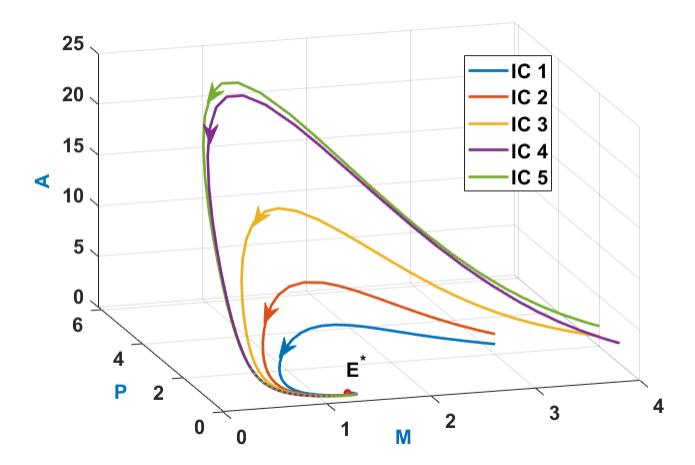
Figure 5: Stability of co-existence equilibrium point \(E^*\) for different parameter values, taken from Table 3. The trajectories are obtained from the system (7) for different initial values of M, P, and A.
5. NUMERICAL SIMULATION AND DISCUSSION
In this section, we have demonstrated the effectiveness of the proposed theoretical results with validation studies from the numerical solution of the atherosclerosis model. The numerical simulations of the model (1)-(6) are carried out with the help of MATHEMATICA software through NDSolve using Runge-Kutta fourth-order method. In various studies [29], [36], [37], we found that the initial conditions are defined as a smooth function of x due to experimentally observed results. Here also we choose the smooth functions of x for the initial conditions, \(M_0(x) = 2 + 2e^{-(0.1x-5)^2}\), \(P_0(x) = 2e^{-(0.1x-5)^2}\) and \(A_0(x) = 2e^{-(0.1x-5)^2}\).
5.1. Numerical Simulation for Non-Inflammatory Equilibrium Point
In this subsection, we discuss the numerical simulation of the model (1)-(6) for the first set of data taken from Table 3. This data has been considered for low concentrations of ox-LDL and cytokines in the intima. Figure 6 clearly shows that initial perturbation in immune cells and cytokines has not impacted. Therefore, the concentration of immune cells, pro, and anti-cytokines rapidly approaches to non-inflammatory equilibrium point \(E_0(2,0,0)\), with the increase of time, which means that the inflammation disappears in a very short time. Hence, we say that the inflammation will vanish if we ensure the inequality \(\frac{\alpha_1}{\lambda_1} < \min\{\frac{\lambda_2}{\alpha_2}, \frac{\lambda_3}{\alpha_3(1-\delta)}\}\) is satisfied.
| Parameters | \(E_0\) | \(E_1\) | \(E^*\) | References |
|---|---|---|---|---|
| \(\alpha_1\) | 2 | 2 | 2 | [29], [36], [37] |
| \(\alpha_2\) | 1 | 1 | 1 | [29], [36], [37] |
| \(\alpha_3\) | 1 | 1 | 2 | [38] |
| \(\beta_1\) | 5 | 1 | 1 | [29] |
| \(\beta_2\) | 1 | 0.2 | 0.2 | Estimated |
| \(\lambda_1\) | 1 | 1 | 1 | [29], [37] |
| \(\lambda_2\) | 4 | 1.8 | 1.8 | Estimated |
| \(\lambda_3\) | 4 | 2 | 2 | Estimated |
| \(\tau_1\) | 1 | 1 | 1 | [29], [37] |
| \(\tau_2\) | \(\frac{42}{43}\) | \(\frac{\frac{42}{43}}{0.2}\) | 1 | [36], [38] |
| \(\delta\) | 0.2 | 0.2 | 0.2 | Estimated |
| \(d_1\) | 1 | 1 | 1 | [29] |
| \(d_2\) | 1 | 1 | 1 | [29] |
| \(d_3\) | 1 | 1 | 1 | [29] |
| \(M_0(x)\) | \[2 + 2e^{-(0.1x - 5)^2}\] | \[2 + 2e^{-(0.1x - 5)^2}\] | \[2 + 2e^{-(0.1x - 5)^2}\] | [37] |
| \(P_0(x)\) | \[2e^{-(0.1x-5)^2} 2e^{-(0.1x-5)^2}\] | \[2e^{-(0.1x-5)^2}\]\[2e^{-(0.1x-5)^2}\] | \[2 + 2e^{-(0.1x-5)^2}\] \[2e^{-(0.1x-5)^2}\] \[2e^{-(0.1x-5)^2}\] | [37] |
| \(A_0(x)\) | \(2e^{-(0.1x-5)^2}\) | \(2e^{-(0.1x-5)^2}\) | \(2e^{-(0.1x-5)^2}\) | [37] |
Table 3: Parameter values for stability at different equilibrium points.
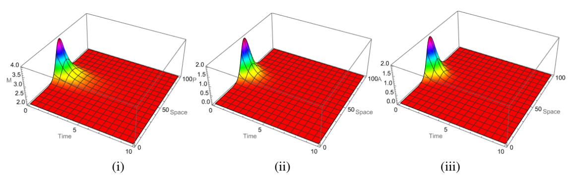
Figure 6: Behaviour of concentration of i) immune cells (M), ii) pro-inflammatory cytokines (P) and iii) anti-inflammatory cytokines with respect to space variable (x) and time (t) for parameter's values taken from Table 3.
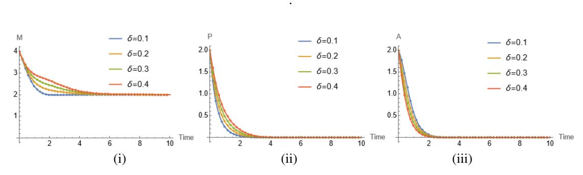
Figure 7: Plot of concentration functions vs. time for different values of \(\delta=0.1,0.2,0.3,0.4\) at x=50 and other parameter's values taken from Table 3.
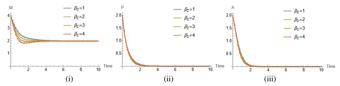
Figure 8: Plot of concentration functions vs. time for different values of β2 = 1, 2, 3, 4 at x = 50 and other parameter's values taken from Table 3.
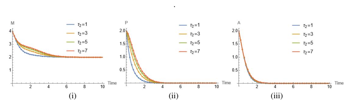
Figure 9: Plot of concentration functions vs. time for different values of τ2 = 1, 3, 5, 7 at x = 50 and other parameter's values taken from Table 3.
Figure 7(i) depicts that the concentration of immune cells decreases over time and tends to α1/λ1, in addition, it increases with the increase of δ. Similarly, Figure 7(ii) shows that the concentration of procytokines decreases over time and tends to 0, and it increases with the increase of δ. However, Figure 7(iii) demonstrates that the concentration of anti-cytokines decreases over time and tends to 0, although it decreases with the increase of δ. In Figure 8(i), it is described that initially the concentration of immune cells decreases exponentially and crosses the level of equilibrium point but as time passes it recovers slowly and reaches the equilibrium point α1/λ1. It is also observed that immune cells decrease with the increase of β2. Similarly, Figures 8(ii) and 8(iii) illustrate that the concentration of both cytokines decreases over time and tends to 0, and they increase slowly with the increase of β2. Figure 9 shows the variation of M and P in a similar fashion as it was plotted for δ. Figure 9(i), the concentration of immune cells has been shown to decrease over time and it tends to α1/λ1, it also assures that the concentration of the same increases with the increase of τ2. Figure 9(ii) shows that the concentration of pro-cytokines decreases over time and tends to 0, and it increases with the increase of τ2. On the other hand, Figure 9(iii) demonstrates that the concentration of anti-cytokines decreases over time and it tends to 0. However, it exhibits almost no variation with the increase of τ2.
5.2. Numerical Simulation for Chronic Equilibrium Point
In this subsection, we discuss the numerical simulation of the model (1)-(6) for the second set of data taken from Table 3. This data stands for high concentration of ox-LDL and moderate concentration of cytokines in the intima, and the above analytical study suggests that this chronic inflammatory point, E1(M1, P1, A1), is stable. Figure 10 evidently demonstrates the behaviour of concentrations with respect to length (x) and time (t). Figure 10(i) shows that initially the immune cells decrease very quickly and drop below the equilibrium level but after some time it recovers and reach the equilibrium point. Figure 10(ii) demonstrates that in a very short time, the concentration of pro-cytokines increases thereafter it decreases over time and tends to equilibrium
point. Figure 10(iii) represents that for the initial time the concentration of pro-cytokines increases thereafter it decreases over time and tends to equilibrium point. So, the numerical simulation assures that the system exhibits a threshold effect to reach its equilibrium point over time. We can see that no anti-inflammatory cytokines exist to suppress the propagation of inflammation. Hence, we say that the inflammation will trigger chronic disease if the inequalities λ1/2 > p K1K2/(K1 + K2) and λ2/α2 < λ3/(α3(1 − δ)) are satisfied.
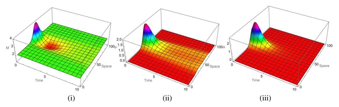
Figure 10: Behavior of concentration of i) Immune cells (M), ii) Pro-inflammatory cytokines (P) and iii) Anti-inflammatory cytokines with respect to space variable (x) and time (t) for values of parameter taken from Table 3.
.
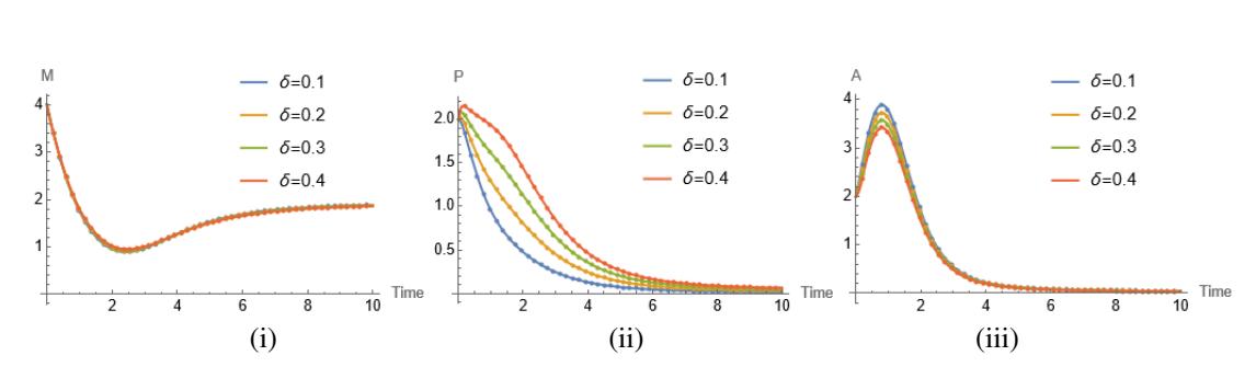
Figure 11: Plot of concentration functions vs. time for different values of δ = 0.1, 0.2, 0.3, 0.4 at x = 50 and other parameter's values taken from Table 3.
.
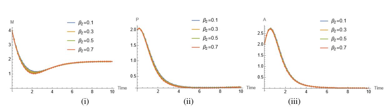
Figure 12: Plot of concentration functions vs. time for different values of β2 = 0.1, 0.3, 0.5, 0.7 at x = 50 and other parameter's values taken from Table 3.
.
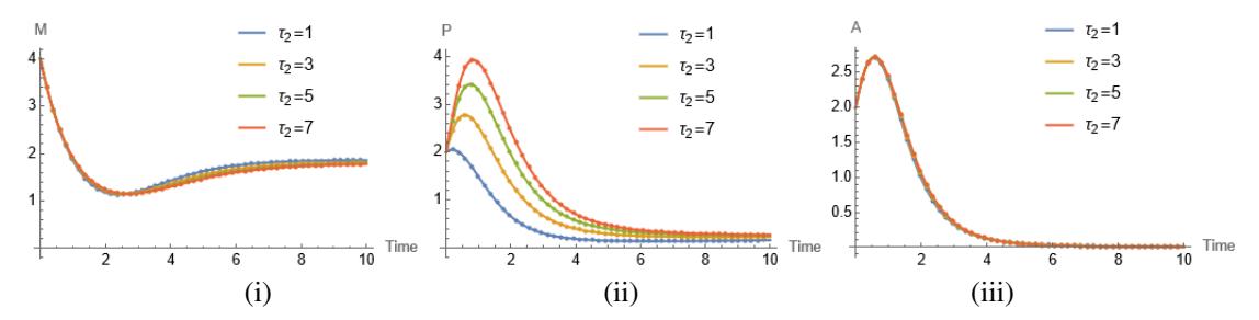
Figure 13: Plot of concentration functions vs. time for different values of \(\tau_2 = 1, 3, 5, 7\) at x = 50 and other parameter's values taken from Table 3.
Figure 11(i) shows that the concentration of immune cells decreases over time and goes down to a certain depth and then it increases and it tends to \(M_1\), but it exhibits almost no variation with the increase of \(\delta\). In Figure 11(ii), the concentration of pro-cytokines gives a little hike and very soon it decreases over time and eventually approaches to \(P_1\), however, it increases with the increase of \(\delta\). Also, Figure 11(iii) demonstrates that the concentration of anti-cytokines first increases very fast for a certain time then it decreases and tends to \(A_1\), although it decreases with the increase of \(\delta\). Figure 12(i) displays that the concentration of immune cells decreases very quickly and drops below the equilibrium level then again after some time it rises and reaches to \(M_1\). Yet, the concentration increases with the increase of \(\beta_2\). In Figure 12(ii), the pro-cytokines initially increase a little bit and very soon decrease and eventually approach to over time, also it decays in very small quantity with the increase of \(\beta_2\). On the other hand, Figure 12(iii) reveals that the concentration of anti-inflammatory cytokines primarily increases for a certain time, then it decreases and tends to \(A_1\). However, it exhibits almost no variation with the increase of \(\beta_2\). In Figure 13(i), it is described that initially the concentration of immune cells decreases and crosses the level of equilibrium point but as time spends it upturns and reaches the equilibrium point \(M_1\). It is also detected that immune cells decrease with the increase of \(\tau_2\). Unlike, Figure 13(ii) shows that the concentration of pro-cytokines initially upturns and tends to \(P_1\) over time and it increases with the increase of \(\tau_2\). On the other hand, Figure 13(iii) does not show any variation in the concentration of anti-inflammatory cytokines with the increase of \(\tau_2\). But the curve initially rises then steadily decays over time and tends to \(A_1\).
5.3. Numerical Simulation of Coexistence Equilibrium Point
In this subsection, the numerical simulation of the presented inflammatory model is displayed for the third set of data of Table 3. This data set corresponds to the medical condition with a high concentration of ox-LDL, medium concentration of pro-inflammatory cytokines, and high concentration of anti-cytokines in the intima. The analytical study assures that this coexistence equilibrium point \(E^*(M^*, P^*, A^*)\) is stable if \(\delta < 0.5\). This coexistence state \(E^*\) is the most concerned equilibrium point in this study. The behaviour of concentration with respect to length (x) and time (t) is shown clearly in Figure 14. Figure 14(i) describes that initially the concentration of immune cells decreases very quickly and drops below the equilibrium level but after some time it recovers and reaches the equilibrium point \(M^*\). Figure 14(ii) demonstrates that in a very short time, the concentration of pro-cytokines increases thereafter it decreases over time and tends to equilibrium point \(P^*\). Figure 14(iii) represents that initially the concentration of pro-cytokines increases thereafter it decreases over time and tends to equilibrium point \(A^*\). If we choose \(\delta > 0.5\), for the same set of data the scenario will be different. In Figure 15, it is shown that the concentrations do not tend to \(E^*(M^*, P^*, A^*)\), rather it approaches to choric equilibrium point \(E_1(M_1, P_1, A_1)\). Figure 14(i) expresses that the concentration of immune cells decreases over time and goes down to a certain level and then it increases. Eventually, it tends to \(M^*\), while \(\delta > 0.5\) and approaches to \(M_1\) for \(\delta > 0.5\).
Moreover, the concentration increases with the increase of \(\delta\). In Figure 15(ii), the concentration of procytokines at first increases exponentially, and then after an interval of time it decreases in a very opposite manner and ultimately approaches \(P^*\), while \(\delta < 0.5\) and approaches \(P_1\) for \(\delta > 0.5\). However, the same
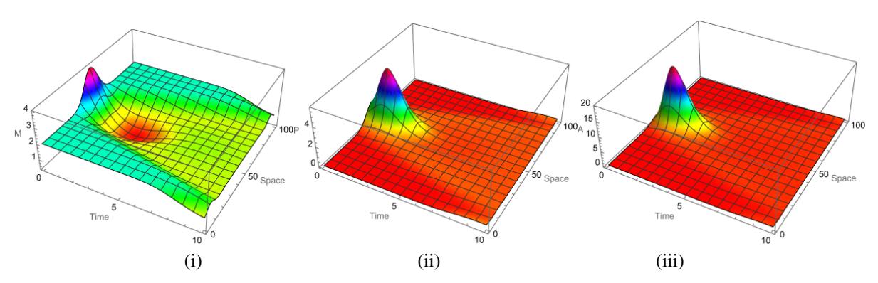
Figure 14: Behavior of concentration of i) Immune cells (M), ii) Pro-inflammatory cytokines (P), and iii) Antiinflammatory cytokines with respect to space variable (x) and time (t) for values of parameter taken from Table 3.
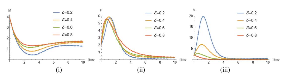
Figure 15: Plot of concentration functions vs. time for different values of δ = 0.2, 0.4, 0.6, 0.8 at x = 50 and other parameter's values taken from Table 3.
.
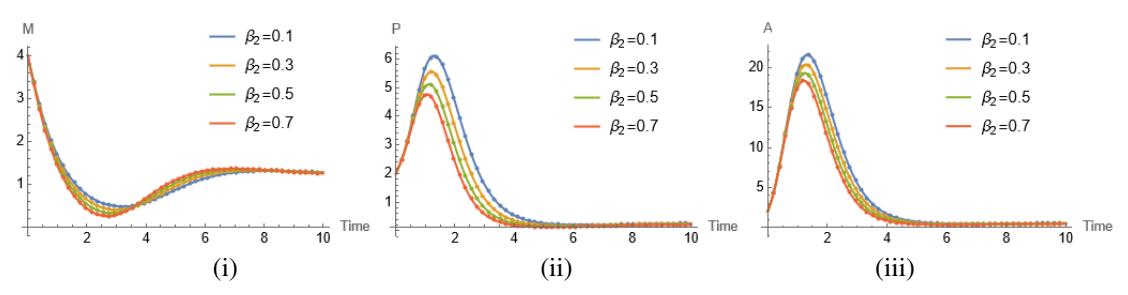
Figure 16: Plot of concentration functions vs. time for different values of β2 = 0.1, 0.3, 0.5, 0.7 at x = 50 and other parameter's values taken from Table 3.
.
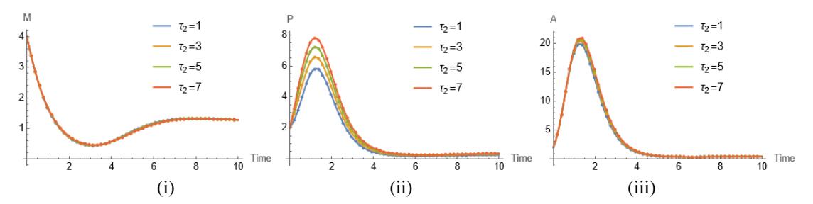
Figure 17: Plot of concentration functions vs. time for different values of \(\tau_2 = 1, 3, 5, 7\) at x = 50 and other parameter's values taken from Table 3.
increases with the increase of \(\delta\). Also, Figure 15(iii) demonstrates that the concentration of anti-cytokines first rises extremely fast up to a high point over time then it decreases and tends to \(A^*\), while \(\delta < 0.5\) and converges to \(A_1\) for \(\delta > 0.5\). Even though it decreases with the increase of \(\delta\). Figure 16(i) displays that the concentration of immune cells decreases very quickly and drops below equilibrium point then after some time it rises. Yet, the concentration decreases initially and then increases with the increase of \(\beta_2\). In Figures 16(ii) and 16(iii) the pro- and anti-inflammatory cytokines initially increase up to a high level and after an interval of time, they both decrease and eventually approach its equilibrium point. Also, they decrease in a very similar fashion with the increase of \(\beta_2\). In Figures 17(i) and 17(iii), immune cells and anti-inflammatory cytokines almost show no variation as \(\tau_2\) increases. But they tend to \(M^*\) and \(A^*\) respectively over time. On the other hand, pro-inflammatory cytokines in Figure 17(ii), grow at a certain level but as time spends decreases and reach \(P^*\). It is also noticed that the concentration of immune cells increases with the increase of \(\tau_2\). Due to the presence of high- high-concentration ox-LDL and high- high-concentration anti-inflammatory cytokines the system has to overcome a threshold effect. This case is very much sensitive to its parameters, especially \(\delta\). Some change of \(\delta\), can make the scenario different. Figure 14 and Figure 18, illustrate this very important fact showing the behavior of concentrations with respect to x and t. We can see for \(\delta = 0.2\), immune cells, pro-inflammatory cytokines, and anti-inflammatory cytokines tend to 1.25, 0.2491, and 0.4743, respectively.
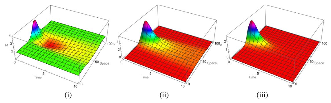
Figure 18: Behavior of concentration of i) Immune cells (M), ii) Pro-inflammatory cytokines (P), and iii) Anti-inflammatory cytokines with respect to space variable (x) and time (t) for \(\delta = 0.6\) values of parameters taken from Table 3.
.
However for \(\delta=0.6\), immune cells, pro-inflammatory cytokines, and anti-inflammatory cytokines tend to 1.8, 0.25, 0, respectively. Hence, we say that \(E^*(1.25, 0.2491, 0.4743)\) will be unable to hold the stability and shift to the chronic inflammatory point \(E_1(1.8, 0.25, 0)\). This transformation of the equilibrium point is shown in a more specific way in Figure 15.
6. CONCLUSIONS
In this article, a reaction-diffusion atherosclerosis model is developed with three different compartments viz. immune cells, pro-inflammatory cytokines, and anti-inflammatory cytokines. This study provides insight into the effects of pro- and anti-inflammatory cytokines in atherosclerosis with the help of a deterministic model. Anti-inflammatory cytokines play an important role in controlling atherosclerosis propagation. But in various studies [27], [28], sometimes few anti-cytokines (TGF-beta, IL-6) have shown opposite characteristics, and behave like pro-inflammatory cytokines. In the proposed model, we consider some anti-cytokines to behave like pro-cytokines, therefore assumed to be there, and denoted with δ. This behavior shows a significant novel impact in this study and provides new insights for the visualization of atherosclerosis. The proposed mathematical model is investigated analytically and numerically. The analytical study suggests that the solutions are unique and stable at non-inflammatory, chronic, and coexistence equilibrium states for a particular set of parameters. Global stability is illustrated through Bellman and Cooke's stability method at the coexistence equilibrium point. We validated and compared analytical results with numerical results [29], [37], which is depicted through Figures 3-18. This study provides three main results; the first one is, that if the intima contains a low concentration of ox-LDL, the dissemination of chronic inflammation does not result from disturbances in the non-inflammatory state, i.e., no chronic inflammation will trigger and the body will recover soon. The second consequence is that when a high concentration of ox-LDL and a moderate concentration of pro and anti-cytokines are present in the intima, inflammation will increase and reach the stage of chronic atherosclerosis. Another possibility is that if a high concentration of ox-LDL, moderate concentration of pro-cytokines, and high concentration of anti-cytokines are available in the intima, inflammation will increase and approach a coexistence equilibrium state and a very less possibility of reaching the stage of chronic atherosclerosis. Hence, a patient will stay alive with the disease in the midst of an uneasy lifestyle. Thus, the results clearly indicate that the patient can avoid the chronic condition if the patient takes a regular and healthy diet with proper medication.
ACKNOWLEDGEMENT
The authors are highly thankful to the unknown referees for their valuable comments and suggestions.