

1. INTRODUCTION
Diabetes mellitus is one of a non-communicable medical condition that cause complex metabolic disorder characterized by hyperglycemia. Hyperglycemia triggers by anomalies of insulin secretion, insulin action, or both ones. The disease can be divided into four main types, i.e., type 1 diabetes mellitus (T1DM), type 2 diabetes mellitus (T2DM), gestational diabetes mellitus (GDM), and diabetes associated with certain specific conditions, e.g., pathologies and disorders [1],[2],[3],[4],[5]. About 5% − 10% diagnosed individuals by diabetes mellitus are the T1DM sufferers. The disease is mainly caused by the damage of pancreatic β cells due to an autoimmune disease that inhibits the insulin production and cause the absence of insulin secretion. The T1DM cases is dominated by children and adolescents [1].
The T2DM, which is also known as non-insulin-dependent diabetes mellitus (NIDDM) or adult-onset diabetes, constitutes about 90% − 95% of all the cases of diabetes. The increasing number of prevalence of T2DM is mainly due to an unhealthy lifestyle [1],[2][3]. The next type of diabetes mellitus is GDM. It is defined as any degree of glucose intolerance or diabetes diagnosed at the outset or during pregnancy. The other form of diabetes, although in smaller percentages with respect to overall diabetic incidence scenario, has been found to be associated with some specific conditions including various pathogens and several disorders. The prominent among those types of diabetes is resulting from the monogenic defects in β-cell function and those due to genetic abnormalities in insulin action, endocrinopathies, exocrine pancreatic pathologies, and several other specific conditions. Based on the causal factors, diabetes which is mostly caused by lifestyle factors is T2DM, see [1],[2],[3],[4],[5].
Diabetes mellitus is also an incurable disease, making proper management and care very important so that the quality of life of diabetes mellitus sufferers is well maintained [6]. Besides diabetes, cardiovascular is also a non-communicable disease. Cardiovascular disease is a disease that occurs due to disruption of blood circulation in the heart and blood vessels. This is caused by the process of atherosclerosis, thrombosis or
∗Corresponding Author
Received November 13th, 2023, Revised January 22nd, 2024 (first), Revised February 25th, 2024 (second), Accepted for publication April 17th, 2024. Copyright ©2024 Published by Indonesian Biomathematical Society, e-ISSN: 2549-2896, DOI:10.5614/cbms.2024.7.1.5
blood clots, and changes in the function of the lining of the arteries [2],[7],[9], [10]. Atherosclerosis comes from high cholesterol in individuals, causing fat buildup and inflammation in the arteries [11].
Unhealthy lifestyle behaviors such as smoking, lack of physical activity, high alcohol consumption, etc., serve as risk factors for both cardiovascular disease and T2DM. The lifestyle behavior is strongly influenced by social networks, which is the social connections that a person has in daily interactions for the exchange of opinions, information, and affection [12], [13]. Obesity can spread within social networks, where it underscores that the connected individuals may share lifestyle factors, such as physical activities and diet, leading to simultaneous weight gain or loss [14],[12],[15].
Furthermore, the similarity in the risk of T2DM throughout social networks can be elucidated by lifestyle behaviors, lifelong socio-economic conditions, or exposure to environmental factors related to diet and physical activity [16]. Type 2 diabetes exhibits characteristics resembling a contagion effect, as it can induce shifts in an individual's lifestyle through social interactions. Trends adopted by communities tend to trigger others to do the same. For example, the consumption of popular sugary beverages normalized this habit. When a new sugary beverage product gained popularity, many people queued and waited for more than half an hour to place their orders. Simultaneously, they influenced other individuals, including family members and friends, to follow suit. With regular consumption of sugary beverages, the pancreas gland's ability to produce insulin may deteriorate over time. Without insulin, human cells cannot effectively utilize glucose, leading to an elevation in blood sugar levels [17]. Unhealthy lifestyles that trigger cardiovascular diseases can also propagate through social interactions. It has been found that cardiovascular risk factors such as obesity and smoking form distinct clusters within social networks, and cardiovascular risk factors spread through social ties in a manner similar to that observed with obesity [18].
Several studies have been carried out on mathematical models of diabetes and complications from diabetes, one of which was discussed by [19]. In [19], the authors analyzed a mathematical model of diabetes mellitus, which is related to the evolution of diabetes to the complications stage but not to the economic, social and medical impacts. The model could be used to monitor the population size of diabetes sufferers and provide the number of sufferers of complications as a function of time. The study in [19] concentrated on nonlinear models and considered the stability analysis of the model's critical points. The results was obtained to estimate the population size of diabetes sufferers and the number of complications over time. In [20], a different mathematical model of diabetes and complications was studied. It was represented mathematically by nonlinear ordinary differential equations, and referred to [19] but with additional cardiovascular population class and a more specific type of diabetes, i.e., T2DM. The model in [20] considered four conditions i.e., obesity without complications, obesity with cardiovascular disease, obesity with type 2 diabetes mellitus (T2DM), and obesity with cardiovascular and T2DM. The study in [20] was focused in predictive models of the cardiovascular disease risk and type 2 diabetes mellitus (T2DM) risk of obese populations. They investigated their impact on the health evolution of obese populations. The authors in [20] shows the role of a healthy lifestyle in alleviating the burden of cardiovascular disease that significantly reduce the risk of developing type 2 diabetes mellitus (T2DM). On the other hand, managing risk factors for obesity with complications greatly reduces the risk of other complications.
In this paper, the authors introduce a new mathematical model of cardiovascular disease and T2DM by adding the social interaction and a susceptible class of individuals who have normal weight. Our model is the extension of the one in [20]. The susceptible class is added based on the fact that not only obese individuals can experience cardiovascular disease and T2DM, but also the individuals with normal weight. We construct a new model of the spread of cardiovascular and T2DM transmissions through social interactions. By using dynamical systems and bifurcation theory, we analyze the transmission of cardiovascular disease and T2DM which spread through social interactions. Our study is focused to understand the role of some parameters to reduce the risk factors of the disease based on the social interactions. We use some bifurcation diagrams to show some scenarios regarding to those situations. This paper is organized as follows: In Section 1 we discuss the introduction of this paper. Model construction and equilibrium points are in Section 2. We explain the stability analysis in Section 3. We discuss bifurcation analysis and numerical simulations in Section 4. Finally, we give the conclusion in Section 5.
2. MODEL FORMULATION
In this section, we consider the construction of a mathematical model of the social interaction between the sufferers of cardiovascular and T2DM. We assume that the population is divided into five compartments i.e., susceptible individuals who have normal weight (N), susceptible individuals who have obesity (O), individuals with cardiovascular disease only (C), individuals with T2DM only (D), individuals with cardiovascular and T2DM complications (G). The total population is represented by P = N + O + C + D + G.
The population is assumed to be homogeneous, and it is closed. The susceptible individuals who have normal weight increases only by the recruitment \((\Lambda)\) only. It means that, the only individuals who have a normal weight and do not suffer from cardiovascular disease or T2DM starting from the age of 40 years who have a risky lifestyle can enter the compartment N. Each sub-population can be reduced due to natural mortality at a rate of \(\mu\). The natural death rate is calculated from the life expectancy starting at age 40. The susceptible individuals who have normal weight can run into obesity if they adopt the lifestyle of obese individuals through social interactions at a rate of \(\eta_1\). On the other hand, individuals who are obese can lose their weight when they interact with vulnerable individuals who have a normal weight due to reducing the risky lifestyle they live due to the influence of social interactions with an interaction level of \(\eta_2\).
Parameters \(\alpha_1\) and \(\alpha_2\), respectively show the rate when the susceptible individuals with normal weight and susceptible individuals with obesity adopt unhealthy lifestyles similar to those of individuals with cardiovascular conditions due to social interactions. When susceptible individuals with normal weight and obese susceptible individuals adopt unhealthy lifestyles similar to those of individuals with T2DM conditions conditions due to social interactions, they may be at risk of developing type 2 diabetes mellitus disease at a rate of \(\beta_1\) and \(\beta_2\), respectively. Social interactions between cardiovascular and T2DM sufferers with mutual influence of unhealthy lifestyles can cause an individual suffer with both cardiovascular and T2DM, with the rate of \(\theta\). The cardiovascular and T2DM disease cannot be cured, so the deaths rate caused by cardiovascular disease is \(\mu_C\).
Individuals with cardiovascular conditions may develop to T2DM due to the progression of risk factors resulting from an unhealthy lifestyle, as observed at a rate of \(\gamma_1\). Individuals with T2DM may experience cardiovascular complications due to the progression of the disease at a rate of \(\gamma_2\). The death of the sufferer of T2DM is usually occurs not directly due to the disease, but it is related to the cardiovascular complications, where the rate is \(\mu_G\).
The transfer diagram of the model represents the spread of cardiovascular and T2DM with social interaction is shown in Figure 1. The formulation of the model is as follows.
\[\frac{dN}{dt} = \wedge + \eta_2 NO - \alpha_1 NC - \eta_1 NO - \mu N - \beta_1 ND,\] \[\frac{dO}{dt} = \eta_1 NO - \alpha_2 OC - \beta_2 OD - \mu O - \eta_2 NO,\] \[\frac{dC}{dt} = \alpha_1 NC + \alpha_2 OC - \gamma_1 C - \mu C - \mu_c C - \theta CD,\] \[\frac{dD}{dt} = \beta_1 ND + \beta_2 OD - \mu D - \gamma_2 D,\] \[\frac{dG}{dt} = \gamma_1 C + \gamma_2 D + \theta CD - (\mu + \mu_G)G.\] (1)
The parameters used in the mathematical model cardiovasscular and type 2 diabetes mellitus are show in Table 2.
3. STEADY STATE CONDITIONS AND BASIC REPRODUCTION NUMBERS
In this section we show how to determine the equilibrium point and we will show the existence of the equilibrium point, then find the basic reproduction number to find out the estimated number of secondary cases of one primary infection in a susceptible population. Next, the stability of each equilibrium point is determined.
3.1. Existence of equilibrium points and basic reproduction numbers
There are seven equilibrium points of System (1). The first one denoted as \((E_1 = (\frac{\wedge}{\mu}, 0, 0, 0, 0))\), is referred to as the disease-free and obesity-free equilibrium point. It exists for all parameter values. The
Figure 1: Transfer diagram of a mathematical model of the social interaction between the sufferers of cardiovascular and type 2 diabetes mellitus.
second equilibrium point, \(E_2=\left(\frac{\mu}{\eta_1-\eta_2},\frac{\wedge}{\mu}-\frac{\mu}{\eta_1-\eta_2},0,0,0\right)\), is called the disease-free and not obese-free equilibrium point. Equilibrium \(E_2\) exists if \(\eta_1>\eta_2\) and \(\frac{\Lambda}{\mu}>\frac{\mu}{\eta_1-\eta_2}\). In this paper, we adopt the concept of basic reproduction number to determine the estimated number of
In this paper, we adopt the concept of basic reproduction number to determine the estimated number of secondary cases of one primary case based on the social interactions in an entirely susceptible population. We apply the next-generation matrix in our system to determine the basic reproduction number, see in [21]. Since system (1) has two disease-free equilibrium points, i.e., disease-free and obesity-free equilibrium point \((E_1)\) and disease-free and not obese-free equilibrium point \((E_2)\), we determine the basic reproduction numbers \((R_{01})\) and \((R_{02})\) as follows.
For \(E_1\), \(R_{01}\) is determined as
\[R_{01} = \max \left\{ \frac{\alpha_1 \wedge}{\mu(\gamma_1 + \mu + \mu_G)}, \frac{\beta_1 \wedge}{\mu(\mu + \gamma_2)} \right\}.\]
For \(E_2\), \(R_{02}\) is determined as
\[R_{02} = \max \left\{ \left( \frac{\alpha_1 \mu}{\eta_1 - \eta_2} + \alpha_2 \left( \frac{\Lambda}{\mu} - \frac{\mu}{\eta_1 - \eta_2} \right) \left( \frac{1}{h} \right) \right), \left( \frac{\beta_1 \mu}{\eta_1 - \eta_2} + \beta_2 \left( \frac{\Lambda}{\mu} - \frac{\mu}{\eta_1 - \eta_2} \right) \left( \frac{1}{\mu + \gamma_2} \right) \right) \right\}.\] where \(h = \gamma_1 + \mu + \mu_G\). The value of \(R_{02}\) is positive if the equilibrium point \(E_2\) exists with the conditions \(\eta_1 > \eta_2\) and \(\frac{\Lambda}{\mu} > \frac{\mu}{\eta_1 - \eta_2}\).
| Notations | Parameters | Units | Value |
|---|---|---|---|
| Λ | Recruitment Population/month | ||
| α1 | Contact social rate between individuals in O and individuals in C | 1/month | 0.05 |
| α2 | Contact social rate between individuals in O and individuals in C | 1/month | 0.1 |
| β1 | Contact social rate between individuals in N and individuals in D | 1/month | 0.04 |
| β2 | Contact social rate between individuals in O and individuals in D | 1/month | 0.2 |
| η1 | Contact social rate between individuals in N and individuals in O | 1/month | 0.4 |
| η2 | Contact social rate between indivuals in O and individuals in N | 1/month | 0.2 |
| µ | natural death rate | 1/month | |
| µC | Death rate from cardiovascular disease | 1/month | 0.03 |
| µG | Death rates from complications of cardiovascular disease and type 2 diabetes mellitus | 1/month | 0.05 |
| γ1 | Rate of development of cardiovascular disease by risk factors | 1/month | 0.4 |
| γ2 | Rate of development of type 2 | 1/month | 0.47 |
| θ | Contact social rate between individuals in C and individuals in D | 1/month | 0.02 |
Table 1: Parameter of mathematical modeling of cardiovascular and type 2 diabetes mellitus with social interaction.
The next equilibrium point is E3 = ( β2D3+µ η1−η2 , ∧ β2D3+µ − β1D3+µ η1−η2 , 0, D3, γ2D3 µ+µG ) where
\[D_3 = \frac{((\gamma_2 + \mu)\mu - \beta_2 \wedge)(\eta_1 - \eta_2) - (\beta_1 - \beta_2)\mu^2}{\beta_2(\mu(\beta_1 - \beta_2) - (\mu + \gamma_2)(\eta_1 - \eta_2))}.\]
The equilibrium represents the cardiovascular-free equilibrium point where the existence is determined by the following conditions:
\[\begin{cases} & \eta_1 > \eta_2, \\ & D_3 > 0, \\ & \frac{\Lambda}{\beta_2 D_3 + \mu} > \frac{\beta_1 D_3 + \mu}{\eta_2 - \eta_2}. \end{cases}\]
Equilibrium point E4 = α2C4+µ η1−η2 , Λ α2C4+µ − α1C4+µ η1−η2 , C4, 0, γ1C4 µ+µG , where C4 = (µ(γ1+µ+µc)−α2Λ)(η1−η2)−µ 2 (α1−α2) α2(µ(α1−α2)−(γ1+µ+µc)(η1−η2)) represents the T2DM-free equilibrium point. It exist for
\[\begin{cases} & \eta_1 > \eta_2, \\ & C_4 > 0, \\ & \frac{\Lambda}{\alpha_2 C_4 + \mu} > \frac{\alpha_1 C_4 + \mu}{\eta_1 - \eta_2}. \end{cases}\]
The other equilibrium points are E5 = µ+γ2 β1 , 0, 0, Λ µ+γ2 − µ β1 , γ2 µ+µG Λ µ+γ2 − µ β1 , that referred to as the obese-free and cardiovascular-free equilibrium point and exists for Λ µ+γ2 > µ β1 , and
\[E_6 = \left(\frac{\gamma_1 + \mu + \mu_c}{\alpha_1}, 0, \frac{\Lambda}{\gamma_1 + \mu + \mu_c} - \frac{\mu}{\alpha_1}, 0, \frac{\gamma_1}{\mu + \mu_G} \left(\frac{\Lambda}{\gamma_1 + \mu + \mu_c} - \frac{\mu}{\alpha_1}\right)\right),\] which is called the obese-free and T2DM-free equilibrium point. Equilibrium E6 exists for Λ γ1+µ+µc > µ α1 .
The last equilibrium is \(E_7 = (N_7, O_7, C_7, D_7, G_7)\), where the components are
\[\begin{split} N_7 &= \frac{-y - \sqrt{y^2 - 4xz}}{2x}, \\ O_7 &= \frac{\Lambda - (\alpha_1 C_7 + \mu + \beta_1 D_7) N_7}{(\eta_1 - \eta_2) N_7}, \\ C_7 &= \frac{(\eta_1 - \eta_2) N_7 - \beta_2 D_7 - \mu}{\alpha_2}, \\ D_7 &= \frac{(\eta_1 - \eta_2) N^2 (\alpha_1 \beta_2 - \alpha_2 \beta_1) + \alpha_2 p_1 (\eta_1 - \eta_2) N}{\beta_2 N (\alpha_1 \beta_2 - \alpha_2 \beta_1)} + \frac{\mu N (\alpha_2 \beta_2 - \alpha_1 \beta_2) - \alpha_2 \beta_2 \Lambda}{\beta_2 N (\alpha_1 \beta_2 - \alpha_2 \beta_1)}, \\ G_7 &= \frac{\gamma_1 C_7 + \gamma_2 D_7 + \theta C_7 D_7}{\mu + \mu_G}, \end{split}\] where \(p_1 = \gamma_2 + \mu\), \(p_2 = \mu + \gamma_1 + \mu_c\), \(x = (\alpha_1\beta_2 - \alpha_2\beta_1)^2 - \theta(\eta_1 - \eta_2)(\alpha_1\beta_2 - \alpha_2\beta_1)\), \(y = (\alpha_1\beta_2 - \alpha_2\beta_1)(\alpha_2(\gamma_2 + \mu) - \beta_2(\mu + \gamma_1 + \mu_c)) + \theta(\beta_2\mu(\alpha_1 - \alpha_2) - \alpha_2(\gamma_2 + \mu)(\eta_1 - \eta_2))\), and \(z = \theta\alpha_2\beta_2\Lambda\). Equilibrium point \(E_7\) is referred to as nontrivial equilibrium point that exist for
\[\begin{cases} \alpha_{1}\beta_{2} > \alpha_{2}\beta_{1}, \\ \theta(\eta_{1} - \eta_{2}) > \alpha_{1}\beta_{2} - \alpha_{2}\beta_{1}, \\ (\eta_{1} - \eta_{2})N_{7} > \beta_{2}D_{7} + \mu, \\ \Lambda > (\alpha_{1}C_{7} + \mu + \beta_{1}D_{7})N_{7}. \end{cases}\]
3.2. Stability analysis
In this section, we consider the stability conditions for each equilibrium point based on the linear analysis of System (1). Our focus are to determine the role of the parameters to obtain the local stability of each equilibrium point of the system.
Theorem 3.1. If \((\eta_1 - \eta_2) \wedge < \mu^2\) and \(R_{01} < 1\), then equilibrium point \(E_1 = (\frac{\wedge}{\mu}, 0, 0, 0, 0)\) of System (1) locally asymptotically stable.
Proof: The eigenvalues of Jacobian matrix of System (1) at \(E_1 = (\frac{\wedge}{\mu}, 0, 0, 0, 0)\) are \(\lambda_1 = -\mu\),
\[\lambda_2 = \frac{(\eta_1 - \eta_2) \wedge}{\mu} - \mu, \tag{2}\]
\[\lambda_3 = \frac{\alpha_1 \wedge}{\mu} - (\gamma_1 + \mu + \mu_c), \tag{3}\]
\[\lambda_4 = \frac{\beta_1 \wedge}{\mu} - (\mu + \gamma_2). \tag{4}\] and \(\lambda_5 = -\mu - \mu_G\). We found that all eigenvalues are negative if \(\frac{(\eta_1 - \eta_2) \wedge}{\mu} < \mu\) or \((\eta_1 - \eta_2) \Lambda < \mu^2, \alpha_1 \Lambda < \mu(\gamma_1 + \mu + \mu_c)\) or \(R_{0A} = \frac{\alpha_1 \wedge}{\mu(\gamma_1 + \mu + \mu_c)} < 1, \beta_1 \Lambda < \mu(\mu + \gamma_2)\) or \(R_{0B} = \frac{\beta_1 \wedge}{\mu(\mu + \gamma_2)} < 1\), then \(E_1\) locally asymptotically stable.
The existence of the disease-free equilibrium point which is locally asymptotically stable can be interpreted that initially, there are several susceptible individuals with normal body weight. Subsequently, there is a small number of susceptible individuals who are obese, another small group suffering from cardiovascular disease, T2DM, and some who have both cardiovascular disease and T2DM. However, over time, the population transitions to a state where only susceptible individuals with normal body weight remain.
Theorem 3.2. If \(R_{02} < 1\) then equilibrium point \(E_2 = (\frac{\mu}{\eta_1 - \eta_2}, \frac{\Lambda}{\mu} - \frac{\mu}{\eta_1 - \eta_2}, 0, 0, 0)\) of System (1) locally asymptotically stable.
Proof: The eigenvalues of Jacobian matrix of System (1) at \(E_2 = (\frac{\mu}{\eta_1 - \eta_2}, \frac{\Lambda}{\mu} - \frac{\mu}{\eta_1 - \eta_2}, 0, 0, 0)\) are
\[\lambda_1 = \frac{\alpha_1 \mu}{\eta_1 - \eta_2} + \alpha_2 \left( \frac{\Lambda}{\mu} - \frac{\mu}{\eta_1 - \eta_2} \right) - (\gamma_1 + \mu + \mu_c), \tag{5}\]
\[\lambda_2 = \frac{\beta_1 \mu}{\eta_1 - \eta_2} + \beta_2 \left( \frac{\Lambda}{\mu} - \frac{\mu}{\eta_1 - \eta_2} \right) - (\mu + \gamma_2), \tag{6}\]
\(\lambda_3 = -\mu - \mu_G, \text{ and } \lambda_{4,5} = \frac{-\frac{\Lambda(\eta_1 - \eta_2)}{\mu} \pm \sqrt{(\frac{\Lambda(\eta_1 - \eta_2)}{\mu})^2 - 4\mu(\eta_1 - \eta_2)\left(\frac{\Lambda}{\mu} - \frac{\mu}{\eta_1 - \eta_2}\right)}}{2}. \text{ We must have } \eta_1 > \eta_2 \text{ and } \frac{\Lambda}{\eta_1 - \eta_2} > \frac{\mu}{\eta_1 - \eta_2} \text{ to satisfy the existence of the } E_2 \text{ and we found that all eigenvalues are negative if } \frac{\alpha_1 \mu}{\eta_1 - \eta_2} + \alpha_2 \left(\frac{\Lambda}{\mu} - \frac{\mu}{\eta_1 - \eta_2}\right) < \left(\gamma_1 + \mu + \mu_c\right) \text{ or } R_{0C} = \left(\frac{\alpha_1 \mu}{\eta_1 - \eta_2} + \alpha_2 \left(\frac{\Lambda}{\mu} - \frac{\mu}{\eta_1 - \eta_2}\right)\right) \left(\frac{1}{\gamma_1 + \mu + \mu_c}\right) < 1, \\ \frac{\beta_1 \mu}{\eta_1 - \eta_2} + \beta_2 \left(\frac{\Lambda}{\mu} - \frac{\mu}{\eta_1 - \eta_2}\right) < (\mu + \gamma_2) \text{ or } R_{0D} = \left(\frac{\beta_1 \mu}{\eta_1 - \eta_2} + \beta_2 \left(\frac{\Lambda}{\mu} - \frac{\mu}{\eta_1 - \eta_2}\right)\right) \left(\frac{1}{\mu + \gamma_2}\right) < 1, \text{ then } E_2 \text{ locally asymptotically stable.}\)
The disease-free and obesity-free equilibrium point which is locally asymptotically stable can be interpreted that initially, the population contains several susceptible individuals who have normal body weight, several susceptible individuals who are obese, a small number of individuals who suffer from cardiovascular disease, a small number of individuals who suffer from T2DM, and a small number of individuals suffer from both cardiovascular and T2DM. However, after some time, this population experiences a change towards a situation where there are no longer any individuals who suffer from cardiovascular disease, T2DM, and suffer from both cardiovascular and T2DM.
Theorem 3.3. If \(\frac{\alpha_1(\beta_2D_3+\mu)}{\eta_1-\eta_2} + \alpha_2\left(\frac{\Lambda}{\beta_2D_3+\mu} - \frac{\beta_1D_3+\mu}{\eta_1-\eta_2}\right) < (\gamma_1 + \mu + \mu_c + \theta D_3), \ P < \sqrt[3]{2}a_2 \ and \ \sqrt[3]{2}B < 2Pa_2\), then equilibrium point \(E_3\) in System (1) locally asymptotically stable, where \(a_1 = 1, \ a_2 = -m_1, \ a_3 = -\beta_2D_3m_7 - m_2m_5 - \beta_1D_3m_4, \ a_4 = \beta_2D_3m_1m_7 - \beta_2D_3m_4m_5 - \beta_1D_3m_2m_7, \ m_1 = -\frac{1}{N_3}, m_2 = -(\beta_2D_3 + \mu), \ m_3 = -\alpha_1N_3, \ m_4 = -\beta_1N_3, \ m_5 = (\eta_1 - \eta_2)O_3, \ m_6 = -\alpha_2O_3, \ m_7 = -\beta_2O_3, \ and \ P = \sqrt[3]{A + \sqrt{A^2 + 4B^3}}, \ A = 9a_2a_3 - 27a_4 - 2a_3^2, \ and \ B = 3a_3 - a_2^2.\)
Proof: Based on the Jacobian matrix at the equilibrium point \(E_4\), it is obtained \(\lambda_1 = -\mu - \mu_G\), \(\lambda_2 = \alpha_1 \left(\frac{\beta_2 D_3 + \mu}{\eta_1 - \eta_2}\right) + \alpha_2 \left(\frac{\Lambda}{\beta_2 D_3 + \mu} - \frac{\beta_1 D_3 + \mu}{\eta_1 - \eta_2}\right) - (\gamma_1 + \mu + \mu_c) - \theta D_3\), and we found characteristic equation is
\[a_1 \lambda^3 + a_2 \lambda^2 + a_3 \lambda + a_4 = 0, (7)\]
where \(a_1=1,\ a_2=-m_1,\ a_3=-\beta_2D_3m_7-m_2m_5-\beta_1D_3m_4,\ a_4=\beta_2D_3m_1m_7-\beta_2D_3m_4m_5-\beta_1D_3m_2m_7,\ m_1=-\frac{1}{N_3}=-\frac{(\eta_1-\eta_2)\Lambda}{\beta_2D_3+\mu}, m_2=-(\beta_2D_3+\mu),\ m_3=-\alpha_1N_3=\frac{-\alpha_1(\beta_2D_3+\mu)}{\eta_1-\eta_2},\ m_4=-\beta_1N_3=\frac{-\beta_1(\beta_2D_3+\mu)}{\eta_1-\eta_2},\ m_5=(\eta_1-\eta_2)O_3=(\eta_1-\eta_2)\left(\frac{\Lambda}{\beta_2D_3+\mu}-\frac{\beta_1D_3+\mu}{\eta_1-\eta_2}\right),\ m_6=-\alpha_2O_3=-\alpha_2\left(\frac{\Lambda}{\beta_2D_3+\mu}-\frac{\beta_1D_3+\mu}{\eta_1-\eta_2}\right),\ m_7=-\beta_2O_3=-\beta_2\left(\frac{\Lambda}{\beta_2D_3+\mu}-\frac{\beta_1D_3+\mu}{\eta_1-\eta_2}\right).\)
By using the Cardano's Formula, see [22], the roots of the polynomial (7) are \(\lambda_3 = \frac{P}{3\sqrt[3]{2}} - \frac{\sqrt[3]{2}B}{3P} - \frac{a_2}{3}\), and \(\lambda_{4,5} = -\frac{P}{6\sqrt[3]{2}} + \frac{\sqrt[3]{2}B}{6P} - \frac{a_2}{3} \pm \frac{i\sqrt{3}}{6} \left(\frac{P}{\sqrt[3]{2}} + \frac{\sqrt[3]{2}B}{P}\right)\) where \(P = \sqrt[3]{A} + \sqrt{A^2 + 4B^3}\), \(A = 9a_2a_3 - 27a_4 - 2a_2^3\), and \(B = 3a_3 - a_2^2\). We must have \(E_3\) exists and so that P is real then \(A^2 + 4B^3 \geq 0\). If \(\alpha_1 \left(\frac{\beta_2 D_3 + \mu}{\eta_1 - \eta_2}\right) + \alpha_2 \left(\frac{\Lambda}{\beta_2 D_3 + \mu} - \frac{\beta_1 D_3 + \mu}{\eta_1 - \eta_2}\right) < (\gamma_1 + \mu + \mu_c) + \theta D_3\), then \(\lambda_2\) is negative, if
\[\frac{P}{3\sqrt[3]{2}} < \frac{a_2}{3} \Leftrightarrow P < \sqrt[3]{2}a_2,\]
then \(\lambda_3\) is negative, and if
\[\frac{\sqrt[3]{2}B}{P} < \frac{a_2}{3} \Leftrightarrow \sqrt[3]{2}B < 2Pa_2,\] then \(Re(\lambda_{4,5})\) is negative, because all the real parts of the values are negative eigenvalues, then \(E_3\) locally asymptotically stable.
The cardiovascular-free equilibrium point which is locally asymptotically stable can be interpreted that initially the population contains some susceptible individuals with normal body weight, some susceptible individuals are obese, a small number suffer from cardiovascular disease, some individuals also suffer from T2DM, and some individuals even experience both cardiovascular disease and T2DM. Furthermore, this population changes its experiences where it lead to a scenario that the individuals do not longer suffer from cardiovascular disease, but they still those who suffer from T2DM, including those with both cardiovascular disease and T2DM.
Theorem 3.4. If \(\frac{\beta_1\Lambda}{(\eta_1-\eta_2)O_4+\alpha_1C_4+\mu}+\beta_2\left(\frac{\Lambda}{\alpha_2C_4+\mu}-\frac{\alpha_1C_4+\mu}{\eta_1-\eta_2}\right)<(\mu+\gamma_2),\ R<\sqrt[3]{2b_2},\ and\ \sqrt[3]{2}C<2Rb_2,\) then equilibrium point \(E_4\) in System (1) locally asymptotically stable, where \(b_1=1,\ b_2=-n_1,\ b_3=-\alpha_1n_3C_4-\alpha_2n_6C_4-n_2n_5,\ b_4=n_1n_6\alpha_2C_4-n_2n_6\alpha_1C_4-n_3n_5\alpha_2C_4,\ n_1=-\frac{1}{N_4},\ n_2=-(\alpha_2C_4+\mu),\) \(n_3=-\alpha_1N_4,\ n_4=-\beta_1N_4,\ n_5=(\eta_1-\eta_2)O_4,\ n_6=-\alpha_2O_4,\ n_7=-\beta_2O_4,\ n_8=\beta_1N_4+\beta_2O_4-(\gamma_2+\mu),\) \(R=\sqrt[3]{C}+\sqrt{C^2+4D^3},\ C=9b_2b_3-27b_4-2b_2^3,\ and\ D=3b_3-b_2^2.\)
Proof: Based on the Jacobian matrix at the equilibrium point \(E_4\), it is obtained \(\lambda_1 = -\mu - \mu_G\), \(\lambda_2 = \beta_1 \left( \frac{\alpha_2 C_4 + \mu}{\eta_1 - \eta_2} \right) + \beta_2 \left( \frac{\Lambda}{\alpha_2 C_4 + \mu} - \frac{\alpha_1 C_4 + \mu}{\eta_1 - \eta_2} \right)\) and we found characteristic equation is
\[b_1 \lambda^3 + b_2 \lambda^2 + b_3 \lambda + b_4 = 0. (8)\] where \(b_1=1, b_2=-n_1, b_3=-\alpha_1 n_3 C_4 - \alpha_2 n_6 C_4 - n_2 n_5, b_4=n_1 n_6 \alpha_2 C_4 - n_2 n_6 \alpha_1 C_4 - n_3 n_5 \alpha_2 C_4, n_1=-\frac{1}{N_4}=-\frac{(\eta_1-\eta_2)\Lambda}{\alpha_2 C_4+\mu}, n_2=-(\alpha_2 C_4+\mu), n_3=-\alpha_1 N_4=-\frac{\alpha_1 (\alpha_2 C_4+\mu)}{\eta_1-\eta_2}, n_4=-\beta_1 N_4=-\frac{\beta_1 (\alpha_2 C_4+\mu)}{\eta_1-\eta_2}, n_5=-(\eta_1-\eta_2)O_4=(\eta_1-\eta_2)\left(\frac{\Lambda}{\alpha_2 C_4+\mu}-\frac{\alpha_1 C_4+\mu}{\eta_1-\eta_2}\right), n_6=-\alpha_2 O_4=-\alpha_2 \left(\frac{\Lambda}{\alpha_2 C_4+\mu}-\frac{\alpha_1 C_4+\mu}{\eta_1-\eta_2}\right), n_7=-\beta_2 O_4=-\beta_2 \left(\frac{\Lambda}{\alpha_2 C_4+\mu}-\frac{\alpha_1 C_4+\mu}{\eta_1-\eta_2}\right), n_8=\beta_1 N_4+\beta_2 O_4-(\gamma_2+\mu)=\beta_1 \left(\frac{\alpha_2 C_4+\mu}{\eta_1-\eta_2}\right)+\beta_2 \left(\frac{\Lambda}{\alpha_2 C_4+\mu}-\frac{\alpha_1 C_4+\mu}{\eta_1-\eta_2}\right)-(\gamma_2+\mu).\)
By using Cardano Formula, see [22], we have the roots of Equation (8) are \(\lambda_3 = \frac{R}{3\sqrt[3]{2}} - \frac{\sqrt[3]{2}D}{3R} - \frac{b_2}{3}\), and \(\lambda_{4,5} = -\frac{R}{6\sqrt[3]{2}} + \frac{\sqrt[3]{2}D}{6R} - \frac{b_2}{3} \pm \frac{i\sqrt{3}}{6} \left(\frac{R}{\sqrt[3]{2}} + \frac{\sqrt[3]{2}D}{R}\right)\) where \(R = \sqrt[3]{C} + \sqrt{C^2 + 4D^3}\), \(C = 9b_2b_3 - 27b_4 - 2b_2^3\), and \(D = 3b_3 - b_2^2\). We must have \(E_4\) exist and so that R is real then \(C^2 + 4B^3 \ge 0\). If
\[\frac{R}{3\sqrt[3]{2}} < \frac{b_2}{3} \Leftrightarrow R < \sqrt[3]{2}b_2\]
then \(\lambda_2\) is negative, and if
\[\frac{\sqrt[3]{2}C}{6R} < \frac{b_2}{3} \Leftrightarrow \sqrt[3]{2}C < 2Rb_2,\] then \(Re(\lambda_{4,5})\) is negative, because all the real parts of the values are negative eigenvalues, then \(E_4\) locally asymptotically stable.
The T2DM-free equilibrium point which is locally asymptotically stable can be interpreted that there are several susceptible individuals who has normal body weight, obese, suffering from cardiovascular disease, a small number suffering from T2DM, and several others even experiencing both cardiovascular disease and T2DM. In this case, the population undergoes to a scenario where individuals are no longer affected by T2DM, but some still suffer from cardiovascular disease, including those with both cardiovascular disease and T2DM
Theorem 3.5. If \(\frac{\Lambda}{\mu+\gamma_2} > \frac{\mu}{\beta_1}\), \(\frac{(\eta_1-\eta_2)(\mu+\gamma_2)}{\beta_1} < \beta_2 \left(\frac{\Lambda}{\mu+\gamma_2} - \frac{\mu}{\beta_1}\right) + \mu\), \(\frac{\alpha_1(\mu+\gamma_2)}{\beta_1} < (\mu+\gamma_2+\mu_c)\), then equilibrium point \(E_5\) in System (1) locally asymptotically stable.
Proof: Based on the Jacobian matrix at the equilibrium point \(E_5\), it is obtained \(\lambda_1 = -\mu - \mu_G\),
\[\lambda_2 = \frac{(\eta_1 - \eta_2)(\gamma_2 + \mu)}{\beta_1} - \beta_2 \left( \frac{\Lambda}{\gamma_2 + \mu} - \frac{\mu}{\beta_1} \right) - \mu, \tag{9}\]
\[\lambda_3 = \frac{\alpha_1(\gamma_2 + \mu)}{\beta_1} - (\gamma_1 + \mu + \mu_c) - \theta \left( \frac{\Lambda}{\gamma_2 + \mu} - \frac{\mu}{\beta_1} \right), \ \lambda_{4,5} = \frac{-\frac{\beta_1 \Lambda}{\gamma_2 + \mu} \pm \sqrt{\left( \frac{\beta_1 \Lambda}{\gamma_2 + \mu} \right)^2 - 4(\beta_1 \Lambda - (\gamma_2 + \mu)\mu)}}{2}.\] We must have \(\frac{\Lambda}{\mu + \gamma_2} > \frac{\mu}{\beta_1}\) to satisfy the existence of the \(E_5\) equilibrium point. If \(\frac{(\eta_1 - \eta_2)(\mu + \gamma_2)}{\beta_1} < \frac{(\eta_1 - \eta_2)(\mu + \gamma_2)}{\beta_1}\)
We must have \(\frac{\Lambda}{\mu+\gamma_2} > \frac{\mu}{\beta_1}\) to satisfy the existence of the \(E_5\) equilibrium point. If \(\frac{(\eta_1-\eta_2)(\mu+\gamma_2)}{\beta_1} < \beta_2 \left(\frac{\Lambda}{\mu+\gamma_2} - \frac{\mu}{\beta_1}\right) + \mu\), so \(\lambda_2\) is negative and if \(\frac{\alpha_1(\mu+\gamma_2)}{\beta_1} < (\mu+\gamma_2+\mu_c)\), so \(\lambda_3\) is negative. Because all the real parts of the values are negative eigenvalues, then \(E_5\) locally asymptotically stable. The obesity-free and cardiovascular-free equilibrium point which is locally asymptotically stable can be
The obesity-free and cardiovascular-free equilibrium point which is locally asymptotically stable can be interpreted that there are several susceptible individuals who have normal body weight, a small number of susceptible individuals who are obese, a small number of others who suffer from cardiovascular disease, and some individuals who suffer from T2DM, and some other individuals even suffer from cardiovascular disease as well as T2DM. The population experiences changes towards a situation that there are no more susceptible individuals who are obese and there are no individuals who suffer from cardiovascular disease but there are still some who suffer from diabetes, and there are still those who suffer from both cardiovascular disease and T2DM
Theorem 3.6. If \(\frac{\Lambda}{\gamma_1 + \mu + \mu_c} > \frac{\mu}{\alpha_1}\), \(\frac{(\eta_1 - \eta_2)(\gamma_1 + \mu + \mu_c)}{\alpha_1} < \mu\) and \(\frac{\beta_1(\gamma_1 + \mu + \mu_c)}{\alpha_1} < (\gamma_1 + \mu)\), then equilibrium point \(E_6\) in System (1) locally asymptotically stable.
Proof: Based on the Jacobian matrix at the equilibrium point \(E_6\), it is obtained
\[\lambda_1 = \frac{(\eta_1 - \eta_2)(\gamma_1 + \mu + \mu_c)}{\alpha_1} - \alpha_2 \left(\frac{\Lambda}{\gamma_1 + \mu + \mu_c} - \frac{\mu}{\alpha_1}\right) - \mu,\tag{10}\]
\(\lambda_2 = \frac{\beta_1(\gamma_1 + \mu + \mu_c)}{\alpha_1} - (\gamma_2 + \mu), \ \lambda_3 = -\mu - \mu_G, \ \text{and} \ \lambda_{4,5} = \frac{-\frac{\alpha_2 \Lambda}{S} \pm \sqrt{(\frac{\alpha_2 \Lambda}{S})^2 - 4(\alpha_1 \Lambda - S \mu)}}{2}, \ \text{where} \ S = \gamma_1 + \mu + \mu_c.\) We must have \(\frac{\Lambda}{\gamma_1 + \mu + \mu_c} > \frac{\mu}{\alpha_1}\) to satisfy the existence of the \(E_6\) equilibrium point. If \(\frac{(\eta_1 - \eta_2)(\gamma_1 + \mu + \mu_c)}{\alpha_1} < \mu\), so \(\lambda_2\) is negative and if \(\frac{\beta_1(\gamma_1 + \mu + \mu_c)}{\alpha_1} < (\gamma_1 + \mu)\), so \(\lambda_3\) is negative. Because all the real parts of the values are negative eigenvalues, then \(E_6\) locally asymptotically stable.
The equilibrium point free from obesity and free from locally asymptotically stable T2DM means that initially there are several susceptible individuals who have normal body weight, a small number of susceptible individuals who are obese, some individuals suffer from cardiovascular disease, a small number of individuals suffer from T2DM, and several other individuals even suffer from both cardiovascular and T2DM. This population experiences changes towards a situation where there are no more susceptible individuals who are obese and there are no individuals who suffer from T2DM but there are still those who suffer from cardiovascular disease and T2DM.
Theorem 3.7. If
- 1) \(k_1 > 0\),
- 2) \(l_1 > 0\),
- 3) \(m_1 > 0\),
\[\begin{array}{lll} e_1 &=& (\eta_2-\eta_1)O_7 - \alpha_1C_7 - \mu - \beta_1D_7, \\ e_2 &=& (\eta_1-\eta_2)N_7 - \alpha_2C_7 - \beta_2D_7 - \mu, \\ e_3 &=& \alpha_1N_7 + \alpha_2O_7 - (\gamma_1+\mu+\mu_c) - \theta D_7, \\ e_4 &=& \beta_1N_7 - \beta_2O_7 - (\mu+\gamma_2), \\ k_1 &=& -e_1 - e_2 - e_3, \\ k_2 &=& (e_1+e_2)e_3 - e_1e_2 + \beta_2^2O_7D_7 - \theta C_7 + \alpha_2^2O_7C_7 + (\eta_1-\eta_2)^2O_7N_7 - (\eta_1-\eta_2)O_7\alpha_2^2C_7N_7 - \alpha_1\alpha_2C_7N_7 - \beta_1^2D_7N_7, \\ k_3 &=& \alpha_2\beta_2\theta O_7C_7D_7 + \alpha_2\beta_2e_4O_7C_7 - \alpha_2^2e_1O_7C_7 - (\eta_1-\eta_2)^2e_3N_7O_7 \\ &+ (\eta_1-\eta_2)\beta_1\beta_2D_7N_7O_7 - \alpha_1\alpha_2(\eta_1-\eta_2)C_7N_7O_7 - \alpha_1\beta_1e_4C_7N_7 + \alpha_1\alpha_2e_2C_7N_7 + \beta_1^2e_3D_7N_7 - \beta_1\beta_2(\eta_1-\eta_2)D_7N_7O_7 - \alpha_2\beta_1\theta C_7D_7N_7 \end{array}\]
(11)
\[\text{[rumus tidak dapat ditampilkan dengan baik — lihat PDF asli]}\] then \(E_7\) in System (1) locally asymptotically stable.
Proof: Based on the Jacobian matrix at the equilibrium point \(E_7\), it is obtained \(\lambda_1 = -\mu - \mu_G\) and we find that the characteristic equation is
\[k_0 \lambda^4 + k_1 \lambda^3 + k_2 \lambda^2 + k_3 \lambda + k_4 = 0, \tag{12}\]
where
\[\text{[rumus tidak dapat ditampilkan dengan baik — lihat PDF asli]}\]
We must have \(E_7\) exists and after obtaining a simpler polynomial function in equation (12), an analysis are carried out using the criteria Routh-Hurwitz, see [23], if \(k_1 > 0\), \(l_1 = \frac{k_1 k_2 - k_3}{k_1} > 0\), and \(m_1 = \frac{l_1 k_3 - k_1 k_4}{l_1} > 0\) that the equilibrium \(E_7\) asymptotically stable.
The nontrivial equilibrium point which is locally asymptotically stable can be interpreted that initially, there are several susceptible individuals with normal body weight, some susceptible individuals who are obese, some individuals suffering from cardiovascular disease, some individuals with T2DM, and some others experiencing both cardiovascular disease and T2DM simultaneously. Over a long period of time, this population has experienced a change towards a situation where there are susceptible individuals who have normal weight, susceptible individuals who are obese, suffer from cardiovascular disease, suffer from T2DM, and suffer from both cardiovascular disease and T2DM.
4. NUMERICAL BIFURCATION ANALYSIS
In this section, we consider bifurcations of System (1) based on the variation of some parameters that involved on the stability criteria as mentioned in Theorem 3.1, Theorem 3.2, Theorem 3.3, Theorem 3.4, Theorem 3.5, Theorem 3.6, and Theorem 3.7. Our analysis is focused to determine the stability regions in the parameter space that can be interpreted as the possible scenarios of the social effects to the population.
A two-parameters bifurcation analysis (Λ and µ) will be conducted by forming a parameter function based on the stability criteria of the equilibrium points. The values of parameters other than Λ and µ are assumed to be fixed. The values of parameter are taken from [20] and some other ones are based on the assumptions.
The parameter values were adopted from [20] are µC = 0.03 that represents a monthly mortality rate of 3 individuals out of 100 from cardiovascular disease, µG = 0.05 that indicates a monthly mortality rate of 5 individuals out of 100 due to complications of cardiovascular disease and T2DM, γ1 = 0.4 that suggests 40 out of 100 individuals with cardiovascular disease may develop T2DM due to risk factors resulting from unhealthy lifestyles, γ2 = 0.47 that indicates 47 out of 100 individuals with T2DM may experience cardiovascular complications as their condition progresses, α2 = 0.1 that reflects 10 out of 100 obese individuals may develop cardiovascular disease due to adopting unhealthy lifestyles through social interactions with individuals who have cardiovascular conditions, and β2 = 0.2 that indicates 20 out of 100 obese individuals may develop T2DM as a result of adopting unhealthy lifestyles influenced by individuals with T2DM.
The parameter values from the assumptions are as follows. Parameter α1 = 0.05 represents 5 out of 100 normal weight individuals experience cardiovascular disease due to unhealthy lifestyle adoption through social interactions with individuals who have cardiovascular conditions, β1 = 0.04 represents 4 out of 100 normal weight individuals develop T2DM influenced by individuals with T2DM through social interactions, η1 = 0.4 represents 4 out of every 100 normal weight individuals become obese due to risky behaviors influenced by obese individuals, η2 = 0.2 represents 2 out of every 100 obese individuals can achieve weight loss by adopting the lifestyle of individuals with normal weight, and θ = 0.02 represents 2 out of 100 individuals with cardiovascular disease develop T2DM by adopting the lifestyle of individuals with T2DM.
In accordance to the existence and stability conditions of the equilibrium point, we focus our study to the role of two parameters, i.e., Λ and µ. Both parameters are appear in the stability conditions of all parameters. By adjusting the values of the remaining parameters, a function involving the variables Λ and µ is established as follows. Based on Equation (2), (3), and (4), for the equilibrium point E1, if λ2 = 0, λ3 = 0, and λ4 = 0, then we have
\[\lambda_{2_{E1}}: \frac{0.2\Lambda - \mu^2}{\mu} = 0, \tag{13}\]
\[\lambda_{3_{E1}}: \frac{0.05\Lambda - 0.43\mu - \mu^2}{\mu} = 0,\] (14)
\[\lambda_{4_{E1}}: \frac{0.04\Lambda - \mu^2 - 0.47\mu}{\mu} = 0. \tag{15}\]
Based on the equation (5) and (6) for the equilibrium E2, if λ1 = 0, and λ2 = 0, then we have
\[\lambda_{1_{E2}}: \frac{0.1\Lambda - 1.25\mu^2 - 0.430\mu}{\mu} = 0,\] (16)
\[\lambda_{2_{E2}}: \frac{0.2\Lambda - 1.8\mu^2 - 0.470\mu}{\mu} = 0.\] (17)
From the equilibrium E5 and E6, we have the eigenvalues (9) and (10). If for E5, λ2 = 0, and for E6, λ1 = 0, then we have
\[\lambda_{2E5}: \frac{9\mu^2 + 6.58\mu + 1.1045 - 0.2\Lambda}{\mu + 0.47} = 0, \tag{18}\]
\[\lambda_{1_{E6}}: \frac{0.7396 + 3.87\mu + 5\mu^2 - 0.1\Lambda}{0.43 + \mu} = 0.\] (19)
Based on the function of parameter on Equations (13), (14), (15), (16), (17), (18), and (19), the bifurcation diagram is obtained in Figure 2.
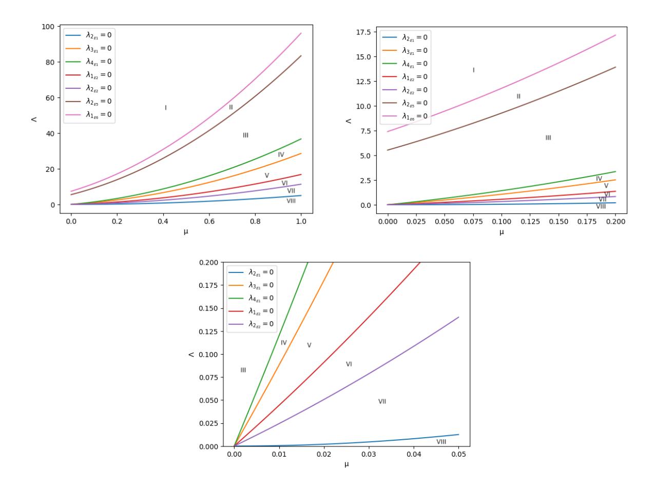
Figure 2: The top-left picture is the bifurcation diagram of the \(\mu\) scale from 0 to 1, the top-right picture is a magnification of the \(\mu\) scale from 0 to 0.2, the bottom picture is a magnification of the \(\mu\) scale from 0 to 0.05.
Figure 2 depicts the bifurcation graph for the Lambda and mu parameters, which shows the existence of 8 regions, namely regions I, II, III, IV, V, VI, VII, and VIII. Region I is bounded by \(\lambda_{1_{E6}}=0\) curve, region II is bounded by \(\lambda_{1_{E6}}=0\) and \(\lambda_{2_{E5}}=0\) curves, region IV is bounded by \(\lambda_{3_{E1}}=0\) and \(\lambda_{3_{E1}}=0\) curves, region V is bounded by \(\lambda_{3_{E1}}=0\) and \(\lambda_{1_{E2}}=0\) curves, region VI is bounded by \(\lambda_{1_{E2}}=0\) and \(\lambda_{2_{E2}}=0\) curves, region VII is bounded by \(\lambda_{2_{E2}}=0\) and \(\lambda_{2_{E1}}=0\) curves, and region VIII is bounded by \(\lambda_{2_{E1}}=0\) curve. Changes in the values of \(\Lambda\) and \(\mu\) when passing through the limiting curve in each region will have a significant impact on the existence and stability of the equilibrium point. A table that describes the eight regions of the bifurcation diagram explicitly is shown in Table 2.
This chapter will discuss the numerical simulation of mathematical modeling of cardiovascular and T2DM with social interaction to illustrate theoretical results and to show the effectiveness and practicability of model, by considering the scenarios of region I until VIII in bifurcation diagram.
4.1. Region I and region II
In region I, parameter values \(\Lambda=8\) means there are 8 million individuals who are entering the age of 40 and have a risky lifestyle and the \(\mu\) parameter value is 0.0042. Based on the parameter values provided in the bifurcation analysis, it is found that there are four equilibrium points exist i.e., \(E_1=(1904.76,0,0,0,0,0)\),
| Region | Equilibrium Existence | Equilibrium Stability |
|---|---|---|
| I | E1, E2, E5, E6 | E5 and E6 asymtotically stable while E1 and E2 is unstable |
| II | E1, E2, E4, E5, E6 | E5 asymtotically stable while E1, E2, E4, E6 is unstable |
| III | E1, E2, E3, E4, E5, E6 | E3 asymtotically stable while E1, E2, E4, E5, E6 is unstable |
| IV | E1, E2, E3, E4, E6 | E3 asymtotically stable while E1, E2, E4, E6 is unstable |
| V | E1, E2, E3, E4 | E3 asymtotically stable while E1, E2, E4 is unstable |
| VI | E1, E2, E3 | E3 asymtotically stable while E1 and E2 is unstable |
| VII | E1, E2 | E2 asymtotically stable while E1 is unstable |
| VIII | E1 | E1 asymtotically stable |
Table 2: Existence and stability regions of the equilibrium points.
E2 = (0.021, 1904.748, 0, 0, 0), E5 = (11.855, 0, 0, 16.766, 145.38), and E6 = (8.684, 0, 18.341, 0, 135.356). Then we obtain R01 = 219 > 1 indicating that the disease-free and obese-free unstable. Besides that, it is also obtained R02 = 803 > 1 so that the equilibrium disease-free but includes obesity unstable. The R02 > R01 value means that at the E2 equilibrium point (where there is an obese subpopulation), the potential for disease spread is greater compared to the E1 equilibrium point (where there are no obese individuals). This indicates that the existence of obese subpopulations can increase the speed of disease spread in the population as a whole. Based on the stability analysis, it is obtained that equilibrium points E5 and E6 are asymptotically stable, while E1 and E2 are unstable.
In region II, parameter values Λ = 6 means that there are 6 million individuals who entering the age of 40 and have a risky lifestyle and the µ parameter value is 0.00379. Based on the parameter values provided in the bifurcation analysis, it is found that there exist four equilibrium points i.e., E1 = (1583.11, 0, 0, 0, 0), E2 = (0.01895, 1583.095, 0, 0, 0), E4 = (6.9, 0.899, 13.76, 0, 102.35), E5 = (11.8, 0, 0, 12.569, 109.825), and E6 = (8.68, 0, 13.76, 0, 102.29).
Then obtained R01 = 182.47 > 1 so that the disease-free and obese-free equilibrium point is unstable. Besides that, it is also obtained R02 = 668, 27 > 1 so that disease-free but not obese-free equilibrium point unstable. The R02 > R01 value means that at the E2 equilibrium point (where there is an obese subpopulation), the potential for disease spread is greater compared to the E1 equilibrium point (where there are no obese individuals). This indicates that the existence of obese subpopulations can increase the speed of disease spread in the population as a whole. Based on the stability analysis, it is obtained that equilibrium points E5 are asymptotically stable, while E1, E2, E4, and E6 are unstable.
The phase portrait projection in region I in the NCD-space are given in the following figure by using initial values x01 = (15, 2, 5, 20, 110), x02 = (13, 5, 4, 25, 140), x03 = (5, 1, 2, 15, 105), x04 = (3, 4, 3, 22, 100),x05 = (10, 5, 15, 10, 115), x06 = (14, 6, 20, 2, 140), x07 = (11, 5, 24, 1, 132), x08 = (4, 1, 12, 0.5, 110), x09 = (8, 2, 8, 1, 100), and x010 = (8, 2, 8, 2.5, 100). The phase portrait projection in region II in the NCD-space are given in the following figure by using initial values x01 = (20, 1, 0.8, 15, 120), x02 = (15, 2, 1, 20, 120), x03 = (17, 1, 0.6, 18, 118), and x04 = (18, 0.6, 1, 16, 119).
In Figure 3 on the left shows that when the initial values x01, x02, x03, x04, x10 are taken, the solution goes to the equilibrium point E5, which means that in this condition there are no susceptible individuals who are obese and no one individual with cardiovascular disease. In this case, for long time there are 11, 855 million susceptible individuals who have normal weight, 16, 766 million individuals who are obese, 145.38 million individuals with type 2 diabetes mellitus, and 145.38 million individuals with suffering from both cardiovascular and T2DM.
On the other hand, when the initial values x05, x06, x07, and x08 are taken, the solution goes to the equilibrium point E6, which means that in this condition there are no susceptible individuals who are obese and no one individual with cardiovascular disease. In this case, for long time there are 8, 684 million susceptible individuals who ave a normal weight, 18, 341 million individuals who are obese, 135, 356 million individuals with suffering from both cardiovascular and T2DM.
In region I to region II there is a change in the number of existing equilibrium points and a change in stability at the equilibrium point E6 from asymptotically stable to unstable. In figure 3 on the right shows that when some initial values are taken around solutions E5, the solutions converges to equilibrium E5, so E5 is asymptotically stable while E1, E2, E4, and E6 unstable. From this conditions it can be concluded that
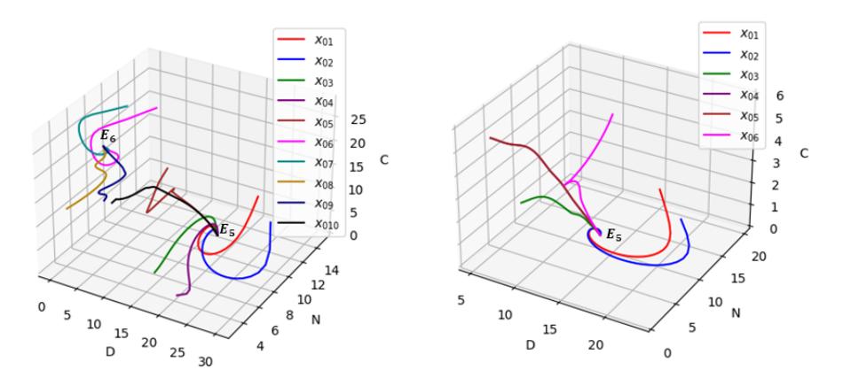
Figure 3: The left picture is the phase portrait projection of System (1) in region I and the right picture is the phase portrait projection of System (1) in region II.
there are no susceptible individuals who are obese and individuals who suffer from cardiovascular disease. In long time, there are 11.8 million susceptible individual who have normal weight, 12.569 million individuals with T2DM, 109.825 million individuals suffering from both cardiovascular disease and T2DM.
4.2. Region III and region IV
In region III, parameter values Λ = 4 means that there are 4 million individuals who entering the age of 40 and have a risky lifestyle and the µ parameter value is 0.00238. Based on the parameter values provided in the bifurcation analysis, it is found that there exist five equilibrium points i.e., E1 = (1680.67, 0, 0, 0, 0), E2 = (0.0119, 1680.66, 0, 0, 0),E3 = (8.434, 0.675, 0, 8.42, 75.57), E4 = (4.619, 2.025, 9.21, 0, 70.37), E5 = (11.81, 0, 0, 8.4083, 75.446), E6 = (8.65, 0, 9.2, 0, 70.28). Then obtained R01 = 194.35 > 1 so that the disease-free and obese-free equilibrium point is unstable. Besides that, it is also obtained R02 = 711, 57 > 1 so that disease-free but not obese-free unstable. Based on the stability analysis, it is obtained that equilibrium points E3 are asymptotically stable, while E1, E2, E4,E5, and E6 are unstable.
In region IV, parameter values Λ = 0.03 means that there are 0.03 million individuals who entering the age of 40 and have a risky lifestyle and the µ parameter value is 0.0033. Based on the parameter values provided in the bifurcation analysis, it is found that there exist five equilibrium points i.e., E1 = (9.09, 0, 0, 0, 0), E2 = (0.0165, 9.07, 0, 0, 0), E3 = (0.063, 2.35, 0, 0.0465, 0.41), E4 = (0.034, 8.28, 0.036, 0, 0.271), and E6 = (8.666, 0, 0.0032, 0, 0.024). Then obtained R01 = 1.049 > 1 so that the disease-free and obese-free equilibrium point is unstable. Besides that, it is also obtained R02 = 3.84 > 1 so that disease-free but not obese-free unstable. Based on the stability analysis, it is obtained that equlibrium points E3 is asymptotically stable, while E1, E2, E4, and E6 unstable.
The phase portrait projection in region III in the NCD-space are given in the following figure by using initial values x01 = (10, 0.7, 0.5, 10, 78), x02 = (8, 0.2, 0.8, 5, 70), x03 = (12, 1, 1, 14, 80), x04 = (11, 0.8, 0.7, 6, 65) dan x05 = (6, 1, 0.2, 5, 70). The phase portrait projection in region IV in the NCDspace are given in the following figure by using initial values x01 = (0.04, 2.8, 0.0002, 0.0185, 0.18), x02 = (0.08, 3, 0.0001, 0.08, 0.5), dan x03 = (0.05, 2.2, 0.0004, 0.15, 0.3).
Figure 4 on the left shows that when some initial values x01, x02, x03, x04, and x05 are taken around the solutions E3 the solutions converges to equilibrium E3 so the equilibrium E3 is asymptotically stable, while E1, E2, E4, E5, and E6 are unstable. In contrast to region II, over an extended period in region III, a susceptible subpopulation of obese individuals coexisted within the population, while individuals with cardiovascular disease are absent from the population. In this scenario, there were 8.434 million susceptible individuals with normal body weight, 0.675 million susceptible obese individuals, 8.42 million individuals with T2DM, and 75.57 million individuals with both cardiovascular and T2DM.
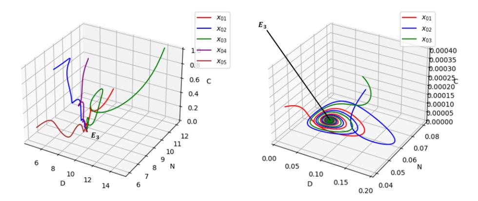
Figure 4: The left picture is the phase portrait projection of System (1) in region III and the right picture is the phase portrait projection of System (1) in region IV.
Figure 4 on the right shows that when some initial values x01, x02, and x03 are taken around the solutions E3. The solutions converges to equilibrium E3 so the equilibrium E3 is asymptotically stable, while E1, E2, E4, and E6 are unstable. The transition from region III to region IV only results in a change in the number of existing equilibrium points. Specifically, the equilibrium point E3 remains locally asymptotically stable, indicating the absence of individuals with cardiovascular in the population, i.e., no one has cardiovascular disease. In this scenario, there are 0.063 million susceptible individuals with normal body weight, 2.35 million susceptible obese individuals, 0.0465 million individuals with T2DM, and 0.41 million individuals suffering from both cardiovascular disease and T2DM.
4.3. Region V and region VI
In region V, parameter values Λ = 0.018 means that there are 0.018 million individuals who entering the age of 40 and have a risky lifestyle and the µ parameter value is 0.00278. Based on the parameter values provided in the bifurcation analysis, it is found that there exist four equilibrium points i.e., E1 = (6.475, 0, 0, 0, 0), E2 = (0.014, 6.461, 0, 0, 0), E3 = (0.0379, 2.356, 0, 0.024, 0.214), dan E4 = (0.021, 13.1, 0.0137, 0, 0.104). Then obtained R01 = 0.75 < 1 but λ1 = 1.29 > 0 at Jacobian in E1 so that the disease-free and obesefree equilibrium point is unstable. Besides that, it is also obtained R02 = 2.73 > 1 so that disease-free but not obese-free unstable. Based on the stability analysis, it is obtained that equilibrium points E3 are asymptotically stable, while E1, E2, E4,E5, and E6 are unstable.
In region VI, parameter values Λ = 0.009 means that there are 0.009 million individuals who entering the age of 40 and have a risky lifestyle and the µ parameter value is 0.00219. Based on the parameter values provided in the bifurcation analysis, it is found that there exist three equilibrium points: E1 = (4.11, 0, 0, 0, 0), E2 = (0.01095, 4.0986, 0, 0, 0), and E3 = (0.019, 2.357, 0, 0.008, 0.07). Then obtained R01 = 0.475 < 1 but λ1 = 0.82 > 0 at Jacobian in E1 so that the disease-free and obese-free equilibrium point is unstable. Besides that, it is also obtained R02 = 1.74 > 1 so that disease-free but not obese-free unstable. Based on the stability analysis, it is obtained that equilibrium points E3 are asymptotically stable, while E1, E2, E4,E5, and E6 are unstable.
The phase portrait projection in region V in the NCD-space are given in the following figure by using initial values x01 = (0.03, 2, 0.0004, 0.01, 0.2) dan x02 = (0.04, 3, 0.0002, 0.05, 0.4). The phase portrait projection in region VI in the NCD-space are given in the following figure by using initial values x01 = (0.0144, 2.32, 0.0003, 0.0034, 0.032), x02 = (0.0149, 2.34, 0.0001, 0.0036, 0.033), and x03 = (0.016, 2.3, 0.0002, 0.005, 0.01).
Figure 5 on the left shows that when some initial values x01 and x02 are taken around the solutions E3, the solutions converges to equilibrium E3 so the equilibrium E3 is asymptotically stable, while E1, E2, and E4 are unstable. From region IV to region V, the number of equilibrium points only changes when the number
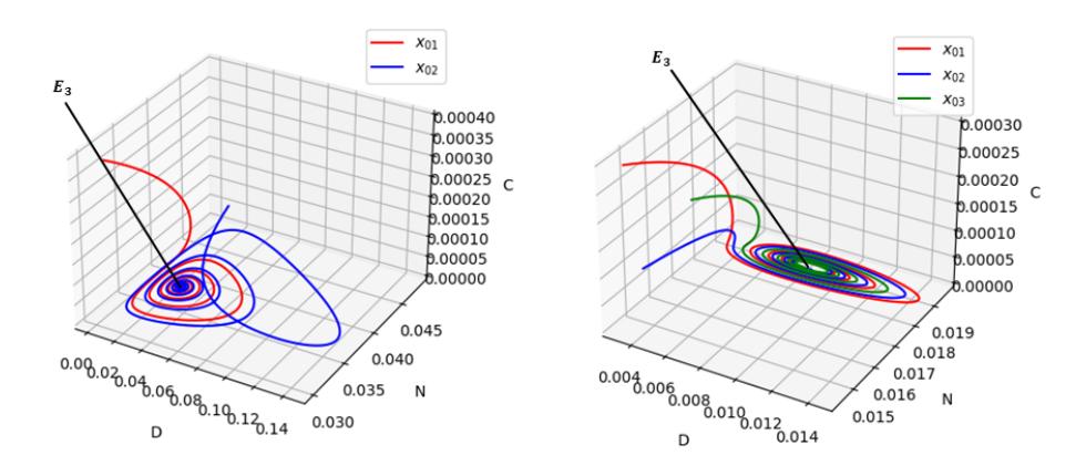
Figure 5: The left picture is the phase portrait projection of System (1) in region V and the right picture is the phase portrait projection of System (1) in region VI.
of recruitment and the natural death rate are changed, while the locally asymptotically stable equilibrium point is the same as in area IV, the equilibrium point E3 where only individuals with cardiovascular disease are absent from the population or in other words there are none who suffer from cardiovascular disease. The recruitment value in area V is smaller than in area IV. In this case, there are 0.0379 million susceptible individuals who have normal body weight, 2.356 million susceptible individuals who are obese, 0.024 million individuals with T2DM, 0.214 million individuals suffering from both cardiovascular and T2DM.
Figure 5 shows that when some initial values x01,x02, and x03 are taken around the solutions E3, the solutions converges to equilibrium E3 so the equilibrium E3 is asymptotically stable, while E1 and E2 are unstable. From region V to region VI the number of existing equilibrium points changes if the number of recruits and natural death rates change, while the locally asymptotically stable equilibrium point is the same as in area V, namely the E3 equilibrium point where only cardiovascular sufferers are missing in the population or in other words there are none who suffer from cardiovascular disease. The recruitment value in area VI is smaller than in area V. In this case there are 0.019 million susceptible individuals who have normal weight, 2.357 million susceptible individuals who are obese, 0.008 million individual with T2DM, and 0.07 million individuals suffering from both cardiovascular and T2DM.
4.4. Region VII and region VIII
In region VII, parameter values Λ = 0.0036 means that there are 0.0036 million individuals who entering the age of 40 and have a risky lifestyle and the µ parameter value is 0.008. Based on the parameter values provided in the bifurcation analysis, it is found that there exist two equilibrium points: E1 = (2.22, 0, 0, 0, 0) and E2 = (0.018, 2.204, 0, 0, 0). Then obtained R01 = 0.256 < 1 but λ1 = 0.44 > 0 at Jacobian in E1 so that the disease-free and obese-free equilibrium point is unstable. Besides that, it is also obtained R02 = 0.932 < 1 so that disease-free but not obese-free asymptotically stable.
In region VIII, parameter values Λ = 0.000025 means that there are 0.000025 million individuals who entering the age of 40 and have a risky lifestyle and the µ parameter value is 0.00238. Based on the parameter values provided in the bifurcation analysis, it is found that there exist one equilibrium points E1 = (0.0105, 0, 0, 0, 0). Then we obtain the value R01 = 0.0012 < 1 and all the eigenvalues of the Jacobian matrix at the equilibrium point E1, i.e., λ1 = −0.00238,λ2 = −0.00011, λ3 = −0.432, λ4 = −0.472, and λ5 = −0.05238 so the equilibrium point E1 is asymptotically stable.
The phase portrait projection in region VII in the NCD-space are given in the following figure by using initial values x01 = (0.0064, 1.58, 0.0002, 0.00012, 0.0001), x02 = (0.006, 1.57, 0.0004, 0.00012, 0.0001), x03 = (0.006, 2, 0.0005, 0.00009, 0.0001), x04 = (0.004, 1.2, 0.0003, 0.00003, 0.0001), and x05 = (0.006, 1.5, 0.0004, 0.00002, 0.0002). The phase portrait projection in region VIII in the NCD-space are given in the following figure by using initial values x01 = (0.011, 0.000011, 0.00001, 0.00001, 0.00001),x02 = (0.012, 0.00001, 0.00001, 0.00002, 0.00001), x03 = (0.011, 0.000012, 0.00001, 0.00002, 0.00003), and x04 = (0.0112, 0.00001, 0.00002, 0.00001, 0.00001).
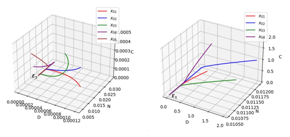
Figure 6: The left picture is the phase portrait projection of System (1) in region VII and the right picture is the phase portrait projection of System (1) in region VIII.
Figure 6 on the left shows that when some initial values x01,x02,x03, x04, and x05 are taken around the solutions E2, the solutions converges to equilibrium E2 so the equilibrium E2 is asymptotically stable, while E1 is unstable. From region VI to region VII there is a change in the number of equilibrium points that exist and there is a change in stability from the unstable equilibrium point E2 in area VI to asymptotically stable in area VII. In this case, over a long period of time there are 0.018 million susceptible individuals who have normal weight and 2.204 million individuals who are obese. From this condition we can infer that in that region is free from diseases. It is nearly an ideal area because in the long term, there is no subpopulation with cardiovascular disease and T2DM, which means that there are no subpopulations with cardiovascular complications and T2DM as well. However, even in this condition, there are individuals who are obese. For this reason, it is necessary to reduce the recruitment rate in order to achieve medically desirable conditions.
Figure 6 on the right shows that when some initial values x01, x02, x03, and x04 are taken around the solutions E1. The solutions converges to equilibrium E1 so the equilibrium E1 is asymptotically stable. from region VII to region VIII there is a change in the number of equilibrium points that exist and there is a change in stability from the unstable E1 equilibrium point in area VII to asymptotically stable in area VIII. In this case, over a long period of time there is only a susceptible subpopulation that has a normal body weight of 0.0105 million individuals. From a medical perspective, the desired outcome is to have no individuals who are obese, suffering from cardiovascular disease, T2DM, or developing cardiovascular complications and T2DM. In Region VIII, the recruitment rate is the lowest among the previous regions. A lower recruitment rate implies that individuals entering the population are mainly those aged 40 and above who lead high-risk lifestyles or are susceptible to unhealthy habits. This, in turn, leads to a reduced number of individuals suffering both from cardiovascular disease and T2DM. Consequently, there is an absence of individuals experiencing cardiovascular complications and T2DM.
5. CONCLUSION
In this paper we examine a mathematical model of the spread of cardiovascular disease and T2DM due to social interactions in populations with risky lifestyles. This model is an extension of the model in [20], by adding the variable of individuals who have normal weight and adding social interactions nfluence individuals in adopting lifestyles. Our model is a first order 5-dimensional ODE system with five variables, namely N, O, C, D, G.
Based on the stability analysis at the equilibrium points, it is known that the system experiences bifurcation when λ = 0. Then the eigenvalue is equal to zero on average containing the parameters Λ and µ so that the parameters Λ and µ play an important role in the stability of an equilibrium point which means that these parameters play an important role in the spread of cardiovascular disease and T2DM through social interactions and we can also find out the role of Λ and µ in reducing the spread of disease.
Based on each region in the bifurcation diagram, a numerical simulation is made in the form of a phase portrait to see the spread of cardiovascular disease or T2DM. In this model, two basic reproduction numbers are found because there are two disease-free equilibrium points but with two different conditions, namely the disease-free and obesity-free equilibrium point (E1) and the disease-free and not obesity-free equilibrium point (E2). In the numerical simulation of each region, it can be seen that in regions I, II, III, IV, V, VI, and VII, it is found that R02 > R01, which means that the spread of cardiovascular disease or T2DM through social interactions is faster when the population contains susceptible individuals who are obese compared to the population when there are none obese individuals. This indicates that the existence of obese subpopulations can increase the speed of disease spread in the population as a whole.
Based on each region in the bifurcation diagram, a numerical simulation was created in the form of a phase portrait to see the spread of cardiovascular disease or T2DM. The numerical simulation for each region found that for parameter values other than Λ and µ the values were fixed so that it is found that the smaller the value of Λ, the obtained R01 < 1, which means that there are no more susceptible individuals who are obese, no more suffer from cardiovascular disease, no more suffer from T2DM, and because in the population no one suffers from cardiovascular disease or T2DM so there are no individuals who suffer from both cardiovascular disease and T2DM. This indicates that the fewer individuals who enter the age of 40 with unhealthy lifestyles, the more cardiovascular disease and T2DM will be lost in that population. On the other hand, as more and more individuals enter the age of 40 with risky lifestyles, cardiovascular disease and T2DM will continue to exist in a population. Prevention must be done from the start before entering the age of 40, even from a young age. The best way for someone who has reached the age of 40 is to maintain a healthy lifestyle such as exercising frequently, avoiding sugary drinks, not smoking or reducing smoking habits, and going on a diet. This healthy lifestyle is also a prevention so that they are not easily influenced by unhealthy lifestyles carried out by obese people, people with cardiovascular disease, or people with T2DM through social interactions. By carrying out bifurcation analysis, conditions can be determined to achieve disease-free and obesity-free conditions in the population in order to reduce the spread of cardiovascular disease and T2DM due to unhealthy lifestyles transmitted through social interactions.