

1. NON-OPTIMAL CONTROL MODEL OF COVID-19 TRANSMISSION DYNAMICS
This section provides a quick overview of the autonomous COVID-19 model, which was thoroughly examined by Peter et al. in [12]. It is worth mentioning that the model does not incorporate mutations. Thus, it is a single but not a multi-strain model like the one studied by the authors in [24], [25], [26], [27] and some of the references cited therein. The model states that the total human population, N, is separated into mutually-exclusive groups of susceptible, S, first-dose vaccinated, V1, second-dose vaccinated, V2, exposed, E, asymptomatic infectious, A, symptomatic infectious, I, hospitalised, H, and recovered, R, people, in a way that at any time t
\[N(t) = S(t) + V_1(t) + V_2(t) + E(t) + A(t) + I(t) + H(t) + R(t).\]
It is pertinent to mention that the detail description of the model's equations is missing in [12]. Thus, we give a full description of the differential equations governing the COVID-19 model previously studied in [12] to showcase the underlying assumptions and its formulation in a more explicit way in this paper as follows.
The susceptible population is generated by birth (or immigration) at a rate θ. The population grows further as a result of the waning of vaccine in first-dose vaccine recipients, making them to become susceptible to the pandemic at a rate τ . It is assumed that the susceptible individuals can contract the disease from individuals in asymptomatic, symptomatic and hospitalized classes. Thus, the population of susceptible human is declined by infection, following the effective contacts with infected humans at a rate λ given by
\[\lambda = \frac{\alpha(\beta_A A + \beta_I I + \beta_H H)}{N}.\tag{1}\]
In (1), α is the effective transmission rate, the parameters 0 < βA, βI , βH < 1 are the modifications parameters, where βA, βI and βH represent the disease transmission reduction rate for infectious humans without symptoms (A), infectious with symptoms (I), and hospitalized humans (H), respectively. As assumed in [12], βA < βH < βI , because the asymptomatic individuals are least infectious since they do not show any symptom of COVID-19, followed by hospitalised individuals who are infectious and currently undergoing treatment, while symptomatic individuals have the highest level of infectiousness as they are not undergoing any treatment yet. Further, the first dose vaccination, administered at a rate ϕ, and natural mortality, occurring at a rate µ, contribute to the population decline. Thus, the evolution of susceptible humans over time is described by
\[\frac{dS}{dt} = \theta + \tau V_1 - \frac{\alpha S(\beta_A A + \beta_I I + \beta_H H)}{N} - \phi S - \mu S.\]
The population of first-dose vaccinated human is generated when the susceptible humans are vaccinated at a rate ϕ. This particular vaccine is assumed to be two-dose without a booster shot. It is decreased due to the waning of the first dose vaccine and administration of the second dose vaccine at rates τ and σ, respectively. Natural mortality further reduces the population at a rate of µ. So, the following differential equation describes how the first-dose vaccination population evolves over time:
\[\frac{dV_1}{dt} = \phi S - \tau V_1 - \sigma V_1 - \mu V_1.\]
The population of the second-dose vaccinated human is generated following the administration of the second dose vaccine, which is assumed to be a particular two-dose vaccine without a booster shot, on the first dose vaccinated humans at a rate σ. It was assumed that the vaccine is perfect [12], so that the second dose vaccinated individuals cannot be re-infected with the disease. Then, the population is decreased following the recovery at a rate η, and further decreases by dying naturally at a rate µ. Thus, the evolution of the second-dose vaccinated population over time is described by
\[\frac{dV_2}{dt} = \sigma V_1 - \eta V_2 - \mu V_2.\]
At a rate λ provided in (1), the susceptible individuals are infected to generate the population of exposed humans. Natural death at a rate of µ and progression to infected classes at a rate of ε both reduce it. Therefore, how the population of exposed human evolves over time is given by
\[\frac{dE}{dt} = \frac{\alpha S(\beta_A A + \beta_I I + \beta_H H)}{N} - \varepsilon E - \mu E.\]
The population of asymptomatic human springs up as a result of the proportion 1− κ of exposed individuals becoming asymptomatically infected at a rate (1 − κ)ε. This population is reduced due to the proportions 1−ρ and ρ developing the disease symptoms and recovering naturally at rates (1−ρ)ψ and ρψ, respectively, and natural death at a rate µ. It was assumed that there is no additional mortality rate for asymptomatic humans due to COVID-19. This is because the asymptomatic individuals do not experience any symptom and assumed not to know their health status in terms of COVID-19. As such, evolution of the asymptomatic human population over time is determined by
\[\frac{dA}{dt} = (1 - \kappa)\varepsilon E - \psi A - \mu A.\]
For the symptomatic infectious human population, it is spring up by the development of clinical symptoms of COVID-19 in exposed and asymptomatic humans at rates κε and (1−ρ)ψ, respectively. The population is scaled down by hospitalization or recovery at rates (1 − b)ω and bω, respectively. The population is further reduced as a result of the respective natural and disease-induced deaths at rates µ and δ. It follows that the symptomatic infectious human population evolves over time as given by
\[\frac{dI}{dt} = \kappa \varepsilon E + (1 - \rho)\psi A - \omega I - \mu I - \delta I.\]
In addition, the population of hospitalized human is generated following the proportion (1−b) of symptomatic infectious individuals being hospitalized at a rate (1 − b)ω. It is reduced when the hospitalized individuals
recover at a rate d. The natural and the disease-induced deaths at rates \(\mu\) and \(\delta\), respectively, further contribute to the decline in the population. Therefore, the evolution of the population of hospitalized human over time is monitored by the differential equation given by
\[\frac{dH}{dt} = (1 - b)\omega I - dH - \mu H - \delta H.\]
Lastly, the compartment for recovered human is populated following the second-dose vaccinated individuals becoming recovered due to vaccine-acquired immunity at a rate \(\eta\). The population is further rose when the asymptomatic, symptomatic and hospitalized humans recover at rates \(\rho\psi\), \(b\omega\) and d, respectively. The population is reduced only due to natural death at a rate \(\mu\). Consequently, how the population of recovered human evolves over time is monitored by the differential equation given as
\[\frac{dR}{dt} = \eta V_2 + \rho \psi + b\omega I + dH - \mu R.\]
In view of the foregoing description, the deterministic model of COVID-19 as presented by the authors of [12], which is an eight-dimensional system of ordinary differential equations, is given by
\[\frac{dS}{dt} = \theta + \tau V_1 - \frac{\alpha S(\beta_A A + \beta_I I + \beta_H H)}{N} - (\phi + \mu)S,\] \[\frac{dV_1}{dt} = \phi S - (\tau + \sigma + \mu)V_1,\] \[\frac{dV_2}{dt} = \sigma V_1 - (\eta + \mu)V_2,\] \[\frac{dE}{dt} = \frac{\alpha S(\beta_A A + \beta_I I + \beta_H H)}{N} - (\varepsilon + \mu)E,\] \[\frac{dA}{dt} = (1 - \kappa)\varepsilon E - (\psi + \mu)A,\] \[\frac{dI}{dt} = \kappa \varepsilon E + (1 - \rho)\psi A - (\omega + \mu + \delta)I,\] \[\frac{dH}{dt} = (1 - b)\omega I - (d + \mu + \delta)H,\] \[\frac{dR}{dt} = \eta V_2 + \rho \psi A + b\omega I + dH - \mu R,\] (2)
with the initial conditions at the initial time t=0 taken as
\[S(0) > 0, V_1(0) > 0, V_2(0) > 0, E(0) > 0, A > 0, I(0) > 0, H > 0, R > 0.\]
In Table 1, we re-present the definitions of the state variables and parameters related to COVID-19 model (2) in the sense of Peter et al. [12].
2. OPTIMAL CONTROL PROBLEM FORMATION FOR DETERMINISTIC COVID-19 MODEL WITH DOUBLE DOSE VACCINATION
This section is devoted to the formulation of the non-autonomous counterpart of the COVID-19 model (2).
2.1. Control state system
The autonomous model of COVID-19 given in (2) is transformed into non-autonomous system with the introduction of five control variables that are time dependent in this part of the paper. Of these five control variables, three are new while the other two were previously taken as constant control rates in model (2). Here is a brief discussion of the five control variables:
- (i) \(u_1(t)\) (previously considered in Model (2) as first dose vaccination with constant rate \(\phi\)) is the control variable representing the efforts of first dose vaccination.
- (ii) \(u_2(t)\) (which was used as a constant second dose vaccination rate \(\sigma\)) is used to measure the second dose vaccination.
Table 1: Description of the models variables and parameters.
| Description | |
|---|---|
| Variable | |
| S | Susceptible humans |
| \(V_1\) | First dose vaccinated humans |
| \(V_2\) | Second dose vaccinated humans |
| E | Exposed humans |
| A | Asymptomatic infected humans |
| I | Symptomatic humans |
| H | Hospitalized humans |
| R | Recovered humans |
| Parameter | |
| \(\beta_A\) | Reduction of transmission rate from asymptomatic to susceptible humans |
| \(\theta\) | Rate of recruitment into the susceptible class |
| \(\mu\) | Natural death rate |
| \(\phi\) | First-dose vaccination rate |
| \(\tau\) | Rate at which the first-dose vaccinated humans progress to the susceptible class |
| \(\alpha\) | Effective transmission rate |
| \(\delta\) | Additional mortality rate due to COVID-19 infection |
| \(\beta_I\) | Reduction of transmission rate from symptomatic to susceptible humans |
| \(\eta\) | Recovery rate induced by the second dose vaccine |
| \(\sigma\) | Second-dose vaccination rate |
| \(\psi\) | Progression rate from asymptomatic infectious compartment |
| \(\rho\) | Fraction of asymptomatic infectious humans who recovered |
| \(\varepsilon\) | Progression rate from exposed class to infectious classes |
| k | Proportion of exposed humans who become symptomatic infectious |
| \(\omega\) | Rate at which individuals leave the symptomatic infected class |
| b | Fraction of symptomatic infectious humans who recovered |
| d | Rate of recovery for hospitalized humans |
| \(\alpha\) | Effective rate of transmission |
| \(\beta_H\) | Reduction of transmission rate from hospitalized to susceptible humans |
- (iii) The preventive measure known as \(u_3(t)\) is intended to stop the spread of the virus from symptomatic, asymptomatic, and hospitalized persons. This can be accomplished by encouraging social distancing, maintaining excellent cleanliness, donning face masks in public locations, and providing healthcare staff with protective equipment.
- (iv) \(u_4(t)\) denotes testing or screening of asymptomatic individuals to detect cases, which enables them to receive the appropriate treatment if they are aware of their health status.
- (v) \(u_5(t)\) represents treatment control variable to enhance the recovery rate of individuals being hospitalized.
Therefore, optimal control model of COVID-19 capturing the aforementioned five time-dependent control variables is represented by the system of ordinary differential equations in (3).
\[\frac{dS}{dt} = \theta + \tau V_1 - \frac{\alpha(1 - u_3(t))S(\beta_A A + \beta_I I + \beta_H H)}{N} - (u_1(t) + \mu)S, \frac{dV_1}{dt} = u_1(t)S - (\tau + u_2(t) + \mu)V_1, \frac{dV_2}{dt} = u_2(t)V_1 - (\eta + \mu)V_2, \frac{dE}{dt} = \frac{\alpha(1 - u_3(t))S(\beta_A A + \beta_I I + \beta_H H)}{N} - (\varepsilon + \mu)E, \frac{dA}{dt} = (1 - \kappa)\varepsilon E - (\psi + u_4(t) + \mu)A, \frac{dI}{dt} = \kappa\varepsilon E + (1 - \rho)\psi A - (\omega + \mu + \delta)I, \frac{dH}{dt} = u_4(t)A + (1 - b)\omega I - (d + u_5(t) + \mu + (1 - u_5(t))\delta)H, \frac{dR}{dt} = \eta V_2 + \rho\psi A + b\omega I + (d + u_5(t))H - \mu R,\] (3)
with the initial conditions taken at time t=0. To help readers understand the model formulation and description better, the flowchart of the non-autonomous COVID-19 model (3) is illustrated in Figure 1.
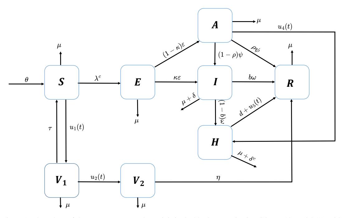
Figure 1: Flow chart of the non-autonomous deterministic double dose vaccination COVID-19 model (3), with \(\delta^c := (1 - u_5(t))\delta\) and \(\lambda^c := \alpha(1 - u_3(t))(\beta_A A + \beta_I I + \beta_H H)/N\).
2.2. Objective functional
Our primary objective is to minimize the numbers of asymptomatic, symptomatic and hospitalized individuals and the costs associated with the application of vaccination, personal protection, screening and treatment as well as to maximize the numbers of first and second dose vaccinated individuals. Then, the following bi-objective functional is defined for the optimal control problem formulation:
\[\mathfrak{J}(u_1, u_2, u_3, u_4, u_5) = \min_{0 \le u_1, u_2, u_3, u_4, u_5} \int_0^{F_t} \left( m_3 A + m_4 I + m_5 H - m_1 V_1 - m_2 V_2 + \frac{1}{2} \left( n_1 u_1^2 + n_2 u_2^2 + n_3 u_3^2 + n_4 u_4^2 + n_5 u_5^2 \right) \right) dt,\] \[(4)\]
where \(m_i, n_i > 0\), i = 1, 2, ..., 5, are the weight constants to minimize the objective functional, the quadratic terms \(\frac{1}{2}n_iu_i^2\) model the non-linearity of the control strategies required to minimize the objective functional (e.g., see [28], [29], [30], [31], [32], [33], [34]), while \(F_t\) denotes the final time for the controls implementation. The weights \(n_i\), i = 1, 2, ..., 5, will depend on the proportionate contribution of each control measure to curbing the disease spread as well as the costs (in terms of human efforts, infrastructural facilities, material resources, among others) associated with putting each one into action per unit time. Thus, the terms \(\frac{1}{2}n_iu_i^2\) (for i = 1, 2, ..., 5) describe the costs associated with first dose vaccination, second dose vaccination, personal protection, screening or testing and treatment, respectively.
In particular, the optimal control problem for the transmission dynamics of COVID-19 is to determine the optimal control quintuple given by \(u^* = (u_i^*), i = 1, 2, ..., 5\), so that
\[\mathfrak{J}(u^*) = \min\{\mathfrak{J}(u_i) : u_i \in \mathfrak{U}\},\tag{5}\]
where \(\mathfrak{U} = \{(u_1(t), u_2(t), u_3(t), u_4(t), u_5(t)) : 0 \leq u_1(t), u_2(t), u_3(t), u_4(t), u_5(t) \leq 1, t \in [0, F_t]\}\) is a non-empty Lebesgue measurable set for the control. Following the existence results due to Fleming and Rishel [35] as applied to optimal control problem models of infectious diseases in [28], [29], [30], [31], it is straightforward to show that the optimal control quintuple \(u^* = (u_1^*, u_2^*, u_3^*, u_4^*, u_5^*)\) exists.
3. ANALYSIS OF THE OPTIMAL CONTROL PROBLEM
3.1. Optimal control characterization
Pontryagin's maximum principle [36] provides the first-order condition to determine the optimal solutions of the control problems. In accordance with this principle, the state system (3) and the objective functional (4) with (5) becomes a problem of minimizing a Hamiltonian \(\mathcal{H}\) defined by (6) pointwise with respect to the time dependent controls \(u_i(t)\), i = 1, 2, ..., 5.
\[\mathcal{H} = \mathfrak{L}(V_1, V_2, A, I, H, u_i) + \lambda_1 \frac{dS}{dt} + \lambda_2 \frac{dV_1}{dt} + \lambda_3 \frac{dV_2}{dt} + \lambda_4 \frac{dE}{dt} + \lambda_5 \frac{dA}{dt} + \lambda_6 \frac{dI}{dt} + \lambda_7 \frac{dH}{dt} + \lambda_8 \frac{dR}{dt},\] (6)
where \(\mathfrak{L}(V_1, V_2, A, I, H, u_i)\) is the Lagrangian of the optimal control problem including the state system (3) and the objective functional (4), which is explicitly defined as
\[\mathfrak{L}(V_1, V_2, A, I, H, u_i) = -m_1 V_1 - m_2 V_2 + m_3 A + m_4 I + m_5 H + \frac{1}{2} \left( n_1 u_1^2 + n_2 u_2^2 + n_3 u_3^2 + n_4 u_4^2 + n_5 u_5^2 \right),\]
\(\lambda_j\), j = 1, 2, ..., 8, denote the adjoint or co-state variables respect to the state variables S, \(V_1\), \(V_2\), E, I, A, H and R. The following theorem gives the necessary conditions for these adjoint variables' existence:
Theorem 3.1. If the optimal control quintuple \(u^* = (u_1^*(t), u_2^*(t), u_3^*(t), u_4^*(t), u_5^*(t))\) minimizes the objective functional (4) over the control set \(\mathfrak U\) subject to the control system (3), then there exist adjoint variables \(\lambda_i\), \(j = 1, 2, \ldots, 8\), satisfying
\[\begin{split} \frac{d\lambda_1}{dt} &= \lambda_1(u_1 + \mu) + \frac{(\lambda_1 - \lambda_4)\alpha(1 - u_3)(\beta_A A + \beta_I I + \beta_H H)}{N} - \lambda_2 u_1, \\ \frac{d\lambda_2}{dt} &= m_1 - \lambda_1 \tau + \lambda_2(\tau + u_2 + \mu) - \lambda_3 u_2, \\ \frac{d\lambda_3}{dt} &= m_2 + \lambda_3(\eta + \mu) - \lambda_8 \eta, \\ \frac{d\lambda_4}{dt} &= \lambda_4(\varepsilon + \mu) - \lambda_5(1 - \kappa)\varepsilon - \lambda_6 \kappa \varepsilon, \\ \frac{d\lambda_5}{dt} &= -m_3 + \frac{(\lambda_1 - \lambda_4)\alpha(1 - u_3)\beta_A S}{N} + \frac{(\lambda_4 - \lambda_1)\alpha(1 - u_3)\beta_A S A}{N^2} + \lambda_5(\psi + u_4 + \mu) - \lambda_6(1 - \rho)\psi \\ &- \lambda_7 u_4 - \lambda_8 \rho \psi, \\ \frac{d\lambda_6}{dt} &= -m_4 + \frac{(\lambda_1 - \lambda_4)\alpha(1 - u_3)\beta_I S}{N} + \frac{(\lambda_4 - \lambda_1)\alpha(1 - u_3)\beta_I S I}{N^2} + \lambda_6(\omega + \mu + \delta) - \lambda_7(1 - b)\omega \\ &- \lambda_8 b\omega, \\ \frac{d\lambda_7}{dt} &= -m_5 + \frac{(\lambda_1 - \lambda_4)\alpha(1 - u_3)\beta_H S}{N} + \frac{(\lambda_4 - \lambda_1)\alpha(1 - u_3)\beta_H S H}{N^2} + \lambda_7(d + u_5 + \mu + (1 - u_5)\delta) \\ &- \lambda_8 (d + u_5), \\ \frac{d\lambda_8}{dt} &= \lambda_8 \mu, \end{split}\]
with transversality conditions
\[\lambda_j(F_t) = 0, \quad j = 1, 2, \dots, 8\] (8)
and the control characterizations
\[\begin{aligned} u_{1}^{*} &= \min \left\{ \max \left\{ 0, \frac{(\lambda_{1} - \lambda_{2})S}{n_{1}} \right\}, 1 \right\}, \\ u_{2}^{*} &= \min \left\{ \max \left\{ 0, \frac{(\lambda_{2} - \lambda_{3})V_{1}}{n_{2}} \right\}, 1 \right\}, \\ u_{3}^{*} &= \min \left\{ \max \left\{ 0, (\lambda_{4} - \lambda_{1}) \frac{\alpha S(\beta_{A}A + \beta_{I}I + \beta_{H}H)}{n_{3}N} \right\}, 1 \right\}, \\ u_{4}^{*} &= \min \left\{ \max \left\{ 0, \frac{(\lambda_{5} - \lambda_{7})A}{n_{4}} \right\}, 1 \right\}, \\ u_{5}^{*} &= \min \left\{ \max \left\{ 0, \frac{(\lambda_{7}(1 - \delta) - \lambda_{8})H}{n_{5}} \right\}, 1 \right\}. \end{aligned}\](9)
Proof: Given that the explicit form of the Hamiltonian H in (6) is
\[\begin{split} \mathcal{H} &= m_3 A + m_4 I + m_5 H - m_1 V_1 - m_2 V_2 + \frac{1}{2} \left( n_1 u_1^2 + n_2 u_2^2 + n_3 u_3^2 + n_4 u_4^2 + n_5 u_5^2 \right) \\ &+ \lambda_1 \left[ \theta + \tau V_1 - \frac{\alpha (1 - u_3(t)) S(\beta_A A + \beta_I I + \beta_H H)}{N} - (u_1(t) + \mu) S \right] \\ &+ \lambda_2 \left[ u_1(t) S - (\tau + u_2(t) + \mu) V_1 \right] + \lambda_3 \left[ u_2(t) V_1 - (\eta + \mu) V_2 \right] \\ &+ \lambda_4 \left[ \frac{\alpha (1 - u_3(t)) S(\beta_A A + \beta_I I + \beta_H H)}{N} - (\varepsilon + \mu) E \right] \\ &+ \lambda_5 \left[ (1 - \kappa) \varepsilon E - (\psi + u_4(t) + \mu) A \right] \\ &+ \lambda_6 \left[ \kappa \varepsilon E + (1 - \rho) \psi A - (\omega + \mu + \delta) I \right] \\ &+ \lambda_7 \left[ u_4(t) A + (1 - b) \omega I - (d + u_5(t) + \mu + (1 - u_5(t)) \delta) H \right] \\ &+ \lambda_8 \left[ \eta V_2 + \rho \psi A + b \omega I + (d + u_5(t)) H - \mu R \right]. \end{split}\]
Then, the co-state system (7) is obtained from solving the following set of equations:
\[\frac{d\lambda_1}{dt} = -\frac{\partial \mathcal{H}}{\partial S}, \quad \frac{d\lambda_2}{dt} = -\frac{\partial \mathcal{H}}{\partial V_1}, \quad \frac{d\lambda_3}{dt} = -\frac{\partial \mathcal{H}}{\partial V_2}, \quad \frac{d\lambda_4}{dt} = -\frac{\partial \mathcal{H}}{\partial E}, \\ \frac{d\lambda_5}{dt} = -\frac{\partial \mathcal{H}}{\partial A}, \quad \frac{d\lambda_6}{dt} = -\frac{\partial \mathcal{H}}{\partial I}, \quad \frac{d\lambda_7}{dt} = -\frac{\partial \mathcal{H}}{\partial H}, \quad \frac{d\lambda_8}{dt} = -\frac{\partial \mathcal{H}}{\partial R},\] with the boundary conditions
\[\lambda_j(F_t) = 0, \ j = 1, 2, \dots, 8.\]
Moreover, the optimal control characterizations in (9) are obtained from solving the following equations:
\[\frac{\partial \mathcal{H}}{\partial u_i} = 0, \ i = 1, 2, \dots, 5. \tag{10}\]
Imposing bounds on the results arising from (10) yields
\[u_i^* = \begin{cases} 0 & \text{if } \vartheta_i \leq 0, \\ \vartheta_i & \text{if } 0 < \vartheta_i < 1, \\ 1 & \text{if } \vartheta_i > 1 \end{cases}\] for i = 1, 2, . . . , 5, and where
\[\begin{split} \vartheta_1 &= \frac{(\lambda_1 - \lambda_2)S}{n_1}, \ \vartheta_2 = \frac{(\lambda_2 - \lambda_3)V_1}{n_2}, \ \vartheta_3 = (\lambda_4 - \lambda_1)\frac{\alpha S(\beta_A A + \beta_I I + \beta_H H)}{n_3 N}, \\ \vartheta_4 &= \frac{(\lambda_5 - \lambda_7)A}{n_4}, \ \vartheta_5 = \frac{(\lambda_7 (1 - \delta) - \lambda_8)H}{n_5}. \end{split}\]
The proof is now complete.
4. SIMULATIONS, RESULTS AND COST-EFFECTIVENESS ANALYSIS
The numerical simulations of the optimality system is covered in this section, along with the costeffectiveness analysis of the specific combinations of the five time-dependent control functions under consideration. The state equations in (3) and their associated initial conditions when t = 0, coupled with the co-state equations (7), the boundary conditions (8), and the characterization of the optimal controls (9), make up the sixteen-dimensional optimality system derived n this paper. The numerical process used to solve this kind of optimality system with various time orientations was described in depth by Lenhart and Workman [37]. In this paper, we coded the numerical process as outlined by the authors in MATLAB.
The parameter values from Table 2 are used with the initial data taken from Peter et al. [12] as S(0) = 32556143, V1(0) = 3, V2(0) = 60, E(0) = 70900, A(0) = 35450, I(0) = 3545, H(0) = 30568 and R(0) = 3331, so that the initial total population at time t = 0 is N(0) = 32700000 to demonstrate the effects of various combinations of at least three of the five optimal control variables on COVID-19 transmission dynamics in a population. For the weight constants in the objective functional (4), we choose the following numbers: mi = 1 (where i = 1, 2, . . . , 5), n1 = 250, n2 = 180, n3 = 150, n4 = 100 and n5 = 120. It should be noted that the weight values used in the simulations are theoretical (not based on real data), having been selected solely to perform the control strategies proposed in this paper.
| Parameter | Value | Unity | Parameter | Value | Unity |
|---|---|---|---|---|---|
| βA | 0.5 | − | βI | 1 | − |
| βH | 0.64 | − | κ | 0.5 | − |
| ψ | 1/15 | day−1 | ω | 1/15 | day−1 |
| θ | 1185 | Humans×day−1 | µ | 1/(75.6 × 365) | day−1 |
| η | 0.1255 | day−1 | τ | 0.0631 | day−1 |
| α | 0.2503 | day−1 | δ | 0.0034 | day−1 |
| ε | 1/5.2 | day−1 | b | 0.7621 | − |
| d | 0.0667 | day−1 | ρ | 0.5314 | − |
Table 2: Parameter values used for simulations (source: [12]).
Since the individuals who received second dose vaccine must have previously received first dose vaccine, all the various combinations involving u2(t) without u1(t) are neglected in the consideration of different possible control combination strategies. On the other hand, it is realistic that people might received the first dose of vaccine and failed to receive the second dose, so combination strategies involving u1(t) without u2(t) are considered. Thus, we take into account various control combination strategies involving the use of at least three different control interventions. These strategies are classified into three main groups, namely, Group A (which includes triple control intervention strategies), Group B (which involves quadruple control interventions) and Group C (which consists of a quintuple control intervention). Specifically, Group A consists of the following seven intervention strategies:
- Strategy A1 Combination of first dose vaccination, u1(t), second dose vaccination, u2(t), and personal protection, u3(t),
- Strategy A2 Combination of first dose vaccination, u1(t), second dose vaccination, u2(t), and testing, u4(t),
- Strategy A3 Combination of first dose vaccination, u1(t), second dose vaccination, u2(t), and treatment, u5(t),
- Strategy A4 Combination of first dose vaccination, u1(t), personal protection, u3(t), and testing or screening, u4(t),
- Strategy A5 Combination of first dose vaccination, u1(t), personal protection, u3(t), and treatment, u5(t),
- Strategy A6 Combination of first dose vaccination, u1(t), testing, u4(t), and treatment, u5(t), and
- Strategy A7 Combination of personal protection, u3(t), testing or screening, u4(t), and treatment, u5(t).
Group B is a set of four control combination strategies, which are:
• Strategy B1 – Combination of first dose vaccination, u1(t), second dose vaccination, u2(t), personal protection, u3(t), and testing, u4(t),
- Strategy B2 Combination of first dose vaccination, u1(t), second dose vaccination, u2(t), personal protection, u3(t), and treatment, u5(t),
- Strategy B3 Combination of first dose vaccination, u1(t), second dose vaccination, u2(t), screening, u4(t), and treatment, u5(t), and
- Strategy B4 Combination of first dose vaccination, u1(t), personal protection, u3(t), screening, u4(t), and treatment, u5(t).
In Group C, there is only one control intervention strategy, henceforth referred to as strategy C, which is all-at-once implementation of the five time-varying control variables.
4.1. Graphical results and their discussions
This section is devoted to the graphical illustrations of the densities of the compartments of the optimal control model (3) with the implementation of the various control combination strategies in Group A, Group B and Group C. In the next three subsections, implementations of the intervention strategies in the three groups, respectively, are taken up.
1) Implementation of the intervention strategies in Group A: Figure 2 shows the impact of implementing an optimal combination of first dose vaccination (u1(t)), second dose vaccination (u2(t)), and personal protection (u3(t)) in order to minimize the objective functional (4). Throughout the intervention period, the sizes of the exposed, infected, and recovered populations in the human population decrease. This reduction is achieved by sustaining the first dose vaccination at its maximal level throughout the intervention, maintaining the second dose vaccination consistently near its minimal level throughout the intervention period, and keeping the optimal personal protection maximally for 150 days, after which it should be gradually lowered to its lowest level by the final time of control implementation period, as depicted in Figure 2(f).
Figure 3 demonstrates the positive impact of a triple intervention comprising an optimal combination of first dose vaccination (u1(t)), second dose vaccination (u2(t)), and testing (u4(t)) in controlling COVID-19. By implementing this strategy, there are significant reductions in the numbers of susceptible, exposed, infected, and recovered individuals. As the control profile in Figure 3(f) indicates, the optimal control u1(t) is consistently maintained maximally throughout the implementation period, optimal control u2(t) is continuously held near the lower bound throughout the implementation period, while the optimal control u4(t) increased from its lower bound and kept at upper bound for 70 days before dropping gradually back to the lower bound at the final time, leading to the observed benefits in disease containment.
Figure 4 illustrates the effectiveness of implementing an optimal combination of first dose vaccination (u1(t)), second dose vaccination (u2(t)), and treatment (u5(t)) to combat COVID-19. The numbers of susceptible, exposed, infected, and recovered individuals have significantly dropped after the implementation this control strategy. According to the control profile in Figure 4(f), the optimal control u1(t) is sustained maximally throughout the intervention period, u2(t) is consistently remained close the lower bound throughout the implementation period, and u5(t) is kept at its upper level for 80 days before dropping gradually to its lower level at the final time Ft = 250 days, contributing to the successful control of the disease.
Figure 5 showcases the impact of implementing an optimal combination of first dose vaccination (u1(t)), personal protection (u3(t)), and testing or screening (u4(t)) in controlling COVID-19. This control intervention results in substantial reductions the numbers of susceptible, exposed, infected, and recovered individuals. The control profile shown in Figure 5(f) shows that while optimal controls u3(t) and u4(t) are respectively held maximally for 130 and 20 days before gradually reducing to their lowest levels at the end of intervention period, optimal control u1(t) is consistently sustained at its highest level over the period of intervention, contributing to the observed beneficial outcomes.
Figure 6 demonstrates the effectiveness of implementing an optimal combination of first dose vaccination (u1(t)), personal protection (u3(t)), and treatment (u5(t)) to control COVID-19. By adopting this strategy, there are significant reductions in the numbers of susceptible, exposed, infected, and recovered individuals. The control profile in Figure 6(f) reveals that the optimal control u1(t) is consistently maintained maximally during the implementation period, while optimal controls u3(t) and u5(t) are held maximally for 150 and 50 days prior to progressively decreasing to their lower bounds during the final intervention period, contributing to the successful control of the disease.
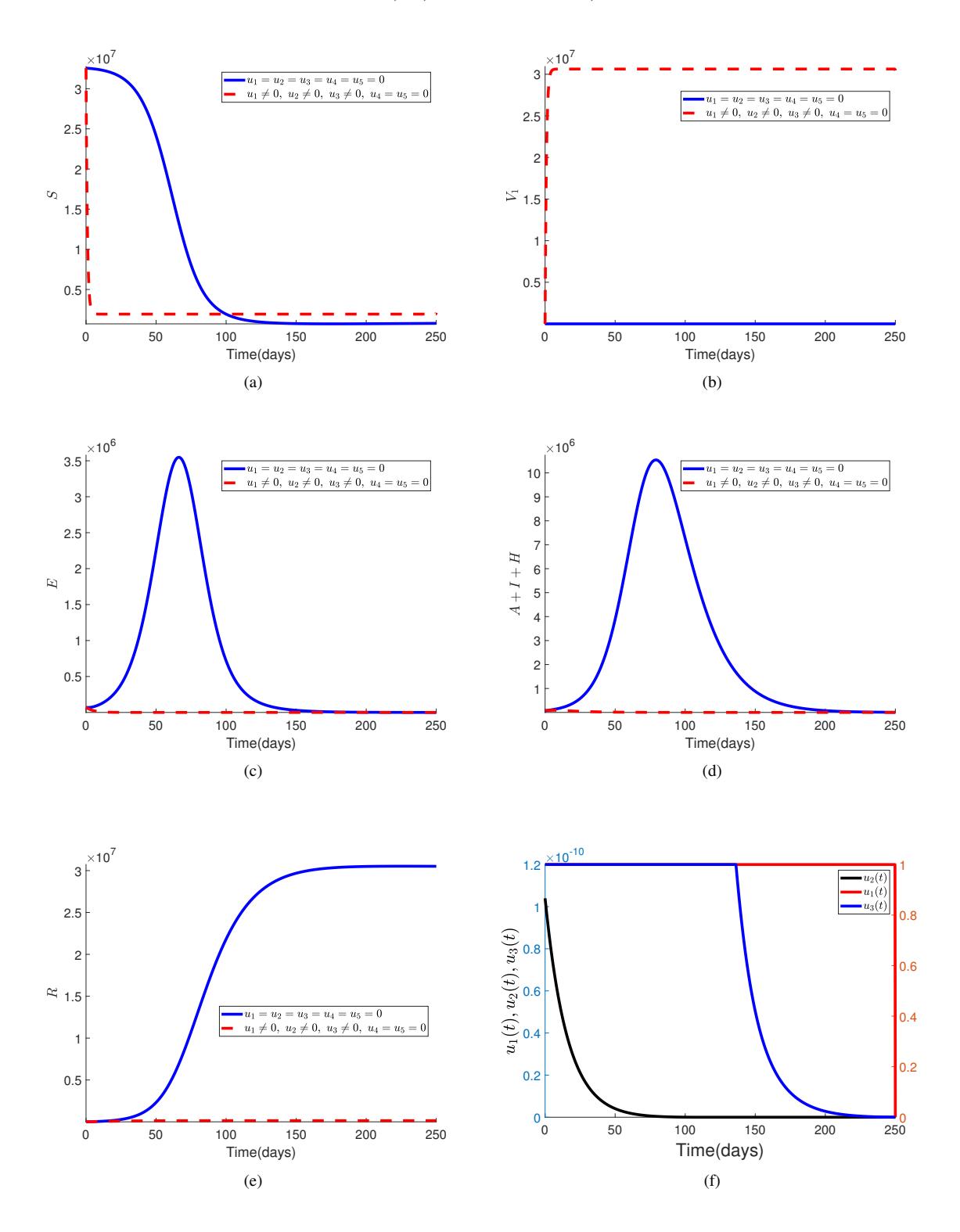
Figure 2: Effect of strategy A1 \((u_1(t), u_2(t), u_3(t))\) on the optimal control COVID-19 model (3).
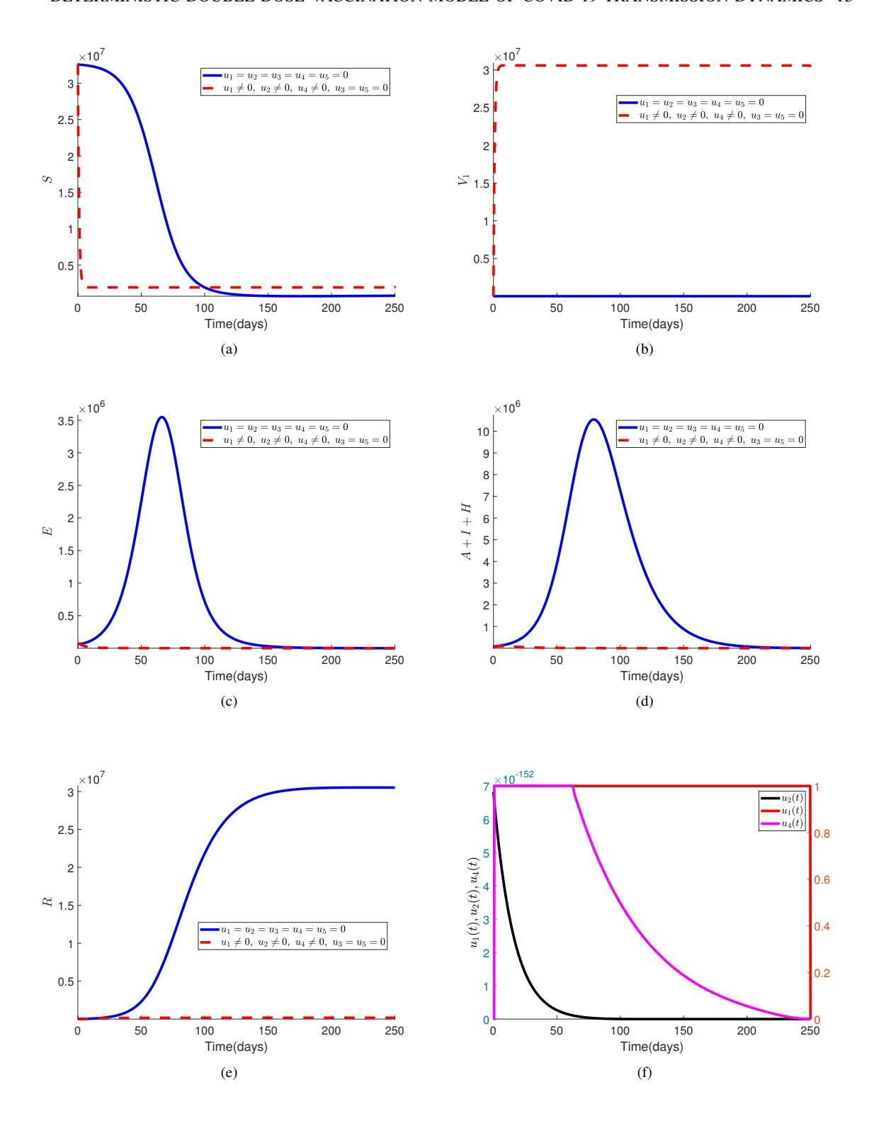
Figure 3: Effect of strategy A2 \((u_1(t), u_2(t), u_4(t))\) on the optimal control COVID-19 model (3).
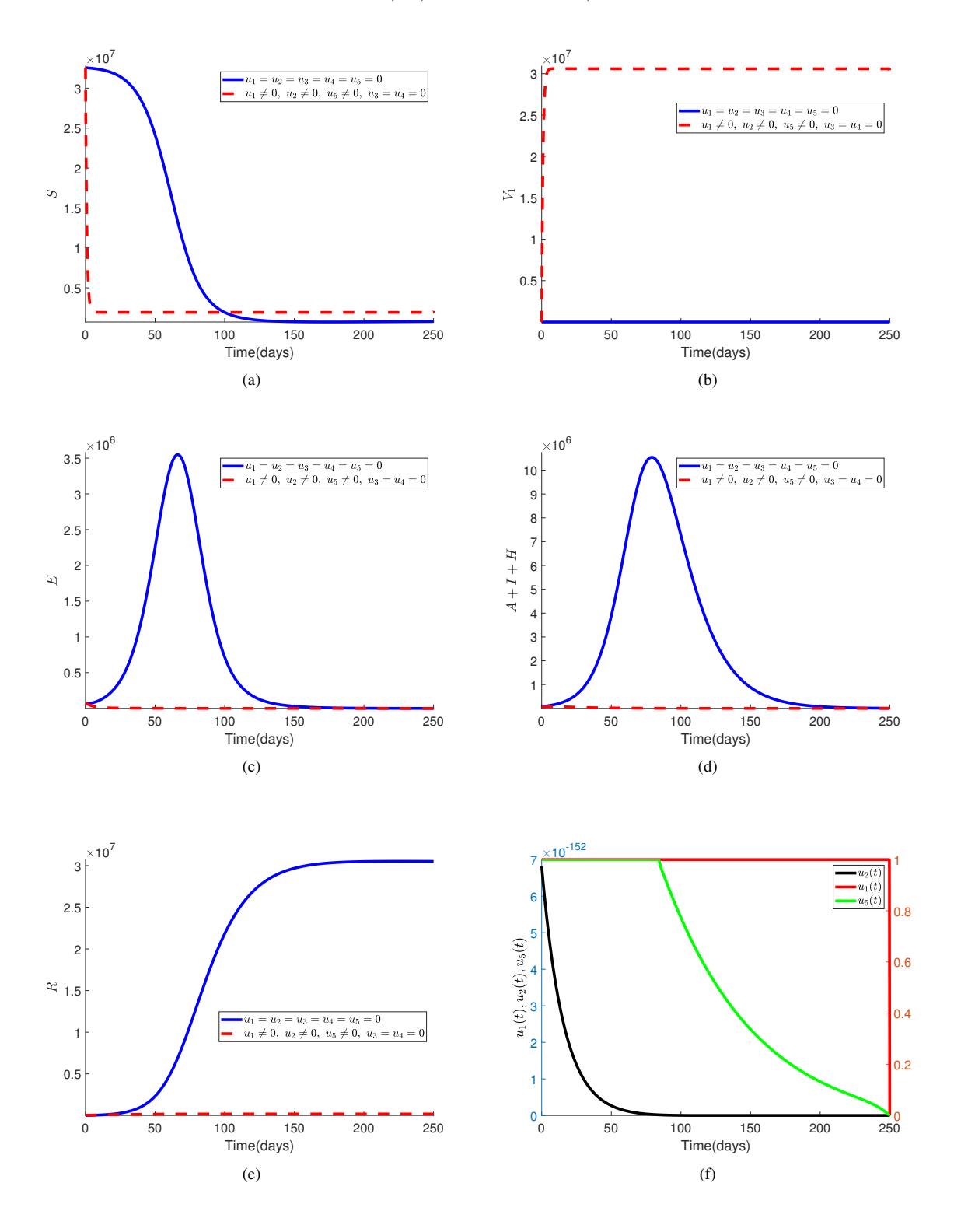
Figure 4: Effect of strategy A3 \((u_1(t), u_2(t), u_5(t))\) on the optimal control COVID-19 model (3).
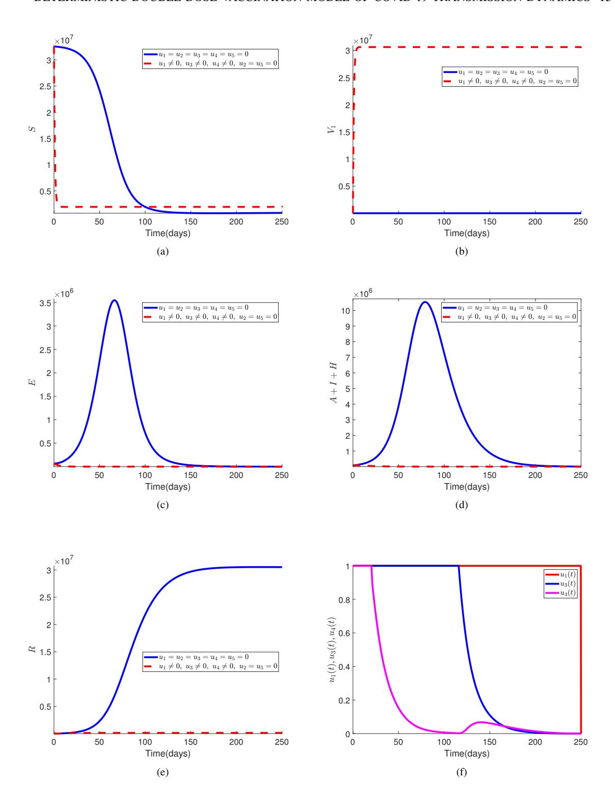
Figure 5: Effect of strategy A4 (u1(t), u3(t), u4(t)) on the optimal control COVID-19 model (3).
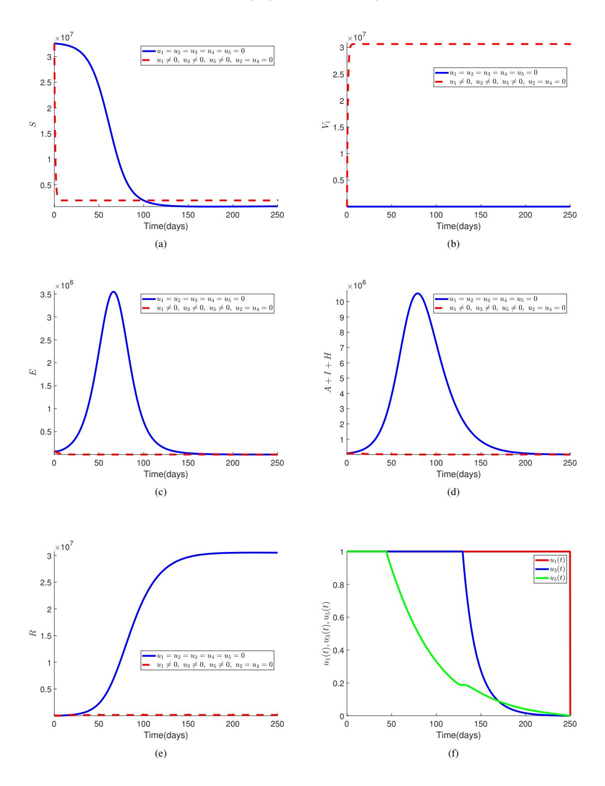
Figure 6: Effect of strategy A5 (u1(t), u3(t), u5(t)) on the optimal control COVID-19 model (3).
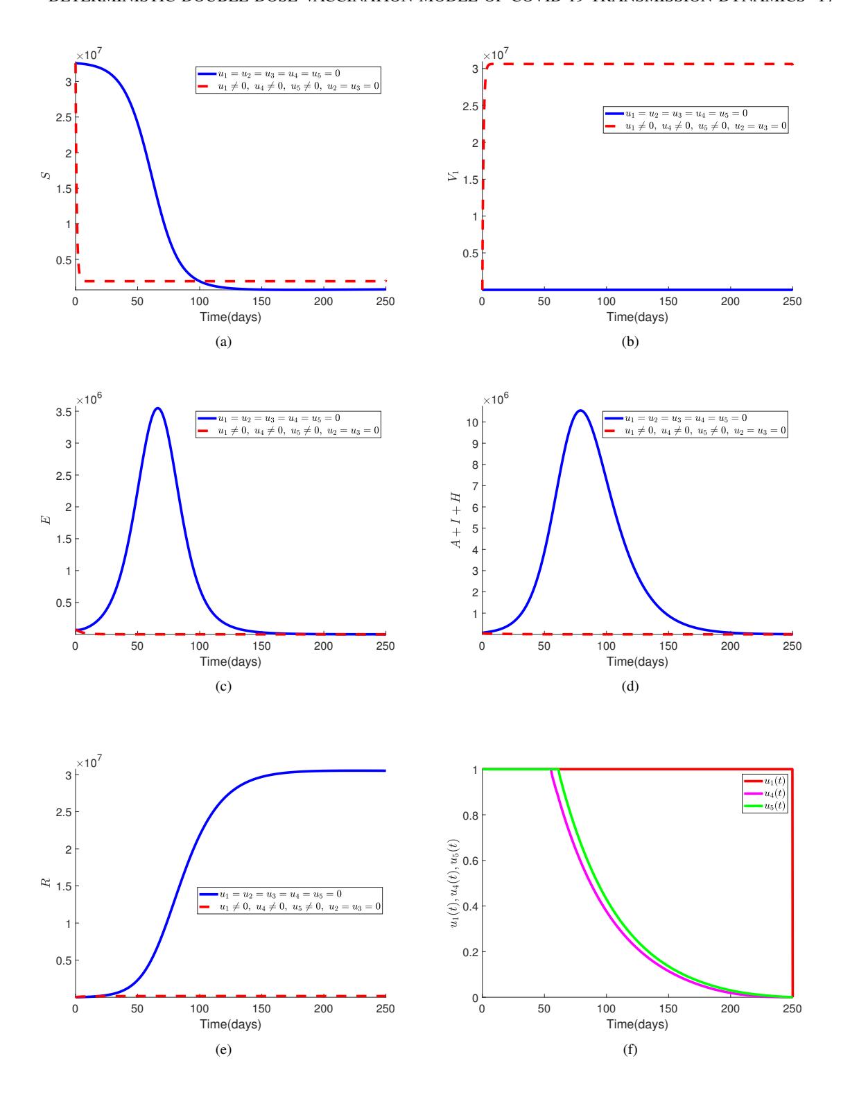
Figure 7: Effect of strategy A6 (u1(t), u4(t), u5(t)) on the optimal control COVID-19 model (3).
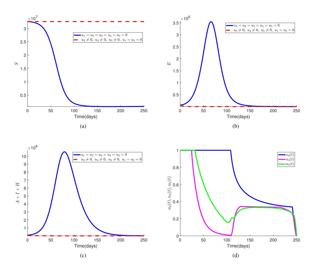
Figure 8: Effect of strategy A7 (u3(t), u4(t), u5(t)) on the optimal control COVID-19 model (3).
In Figure 7, the impact of implementing an optimal combination of first dose vaccination (u1(t)), testing (u4(t)), and treatment (u5(t)) towards the control of COVID-19 is illustrated. This control intervention strategy leads to considerable reductions in the numbers of susceptible, exposed, infected, and recovered individuals. The control profile in Figure 7(f) confirms that the optimal control u1(t) is sustained at its upper bound over the entire intervention period, while the optimal controls u4(t), and u5(t) are consistently sustained at their highest levels for 52 and 55 days, respectively, prior to gradual decrease to their lowest values during the final intervention period, contributing to the successful control of the disease.
Figure 8 showcases the impact of implementing an optimal combination of personal protection (u3(t)), testing or screening (u4(t)), and treatment (u5(t)) in controlling COVID-19. This control intervention leads to significant reductions in the numbers of susceptible, exposed, infected, and recovered individuals. As suggests by the control profile in Figure 8(d), the optimal controls u3(t), u4(t), and u5(t) are consistently maintained at their highest levels for 120, 30 and 50 days, respectively, after which they reduce gradually to their lowest levels during the final time Ft of intervention, contributing to the successful control of the disease.
2) Implementation of the quadruple intervention strategies in Group B: Figure 9 presents the results of the four-control intervention involving an optimal combination of first dose vaccination (u1(t)), second dose vaccination (u2(t)), personal protection (u3(t)), and testing (u4(t)), with the objective of minimizing the functional (4) over the period of implementation. Implementing this strategy is highly effective, leading to the complete elimination of the susceptible, exposed, infected, and recovered populations during the period of intervention. To reach this optimal outcome, it is essential to sustain the optimal control for first-dose vaccination maximally over the intervention period, second-dose vaccination consistently near its lowest level throughout the control implementation period, personal protection and testing at their maximum levels for 120 and 30 days before gradually reducing them to their minimum levels by the end of the implementation period, as depicted in Figure 9(e).
In Figure 10, the optimal combination of first dose vaccination (u1(t)), second dose vaccination (u2(t)), personal protection (u3(t)), and treatment (u5(t)) is utilized to minimize the objective functional (4) over the implementation period of Ft = 250 days. This control intervention proves highly effective in causing the susceptible, exposed, infected, and recovered populations during the course of control implementation. To reach this successful outcome, the optimal first dose vaccination is sustained maximally throughout the intervention period, optimal second dose vaccination is held continuously near its lowest level over the implementation period, while the personal protection and treatment controls are respectively kept at their upper bounds for 130 and 50 days, and thereafter reduced gradually to their lower bounds at the final time of the implementation, as suggested by Figure 10(f).
Figure 11 showcases the implementation of an optimal combination of first dose vaccination (u1(t)), second dose vaccination (u2(t)), screening (u4(t)), and treatment (u5(t)) towards minimizing the objective functional (4) over the time interval t ∈ [0, 250] days of control implementation. By implementing this control intervention, the susceptible, exposed, infected, and recovered populations vanish throughout the period of the control intervention. Achieving this outcome involves sustaining the optimal first dose vaccination at its upper bound over the intervention period, second dose vaccination consistently near its lower level throughout the period of intervention, screening or testing and treatment controls at their highest level for 60 and 70 days, respectively, and thereafter reducing them gradually to their lowest levels at the final time, as shown in Figure 11(f).
In Figure 12, the optimal combination of first dose vaccination (u1(t)), personal protection (u3(t)), screening (u4(t)), and treatment (u5(t)) is utilized with the goal of minimizing the objective functional (4) during the control implementation period. Implementing this strategy leads to the disappearance of the susceptible, exposed, infected, and recovered populations throughout the intervention period. This favourable outcome is achieved when the optimal first dose vaccination is sustained at its maximum level over the entire period of intervention, whereas the optimal personal protection, screening or testing and treatment controls are maintained at their highest levels for 120, 30 and 40 days, respectively, and then reduced gradually to their lowest levels at the final time Ft = 250 days, as suggests by Figure 12(f).
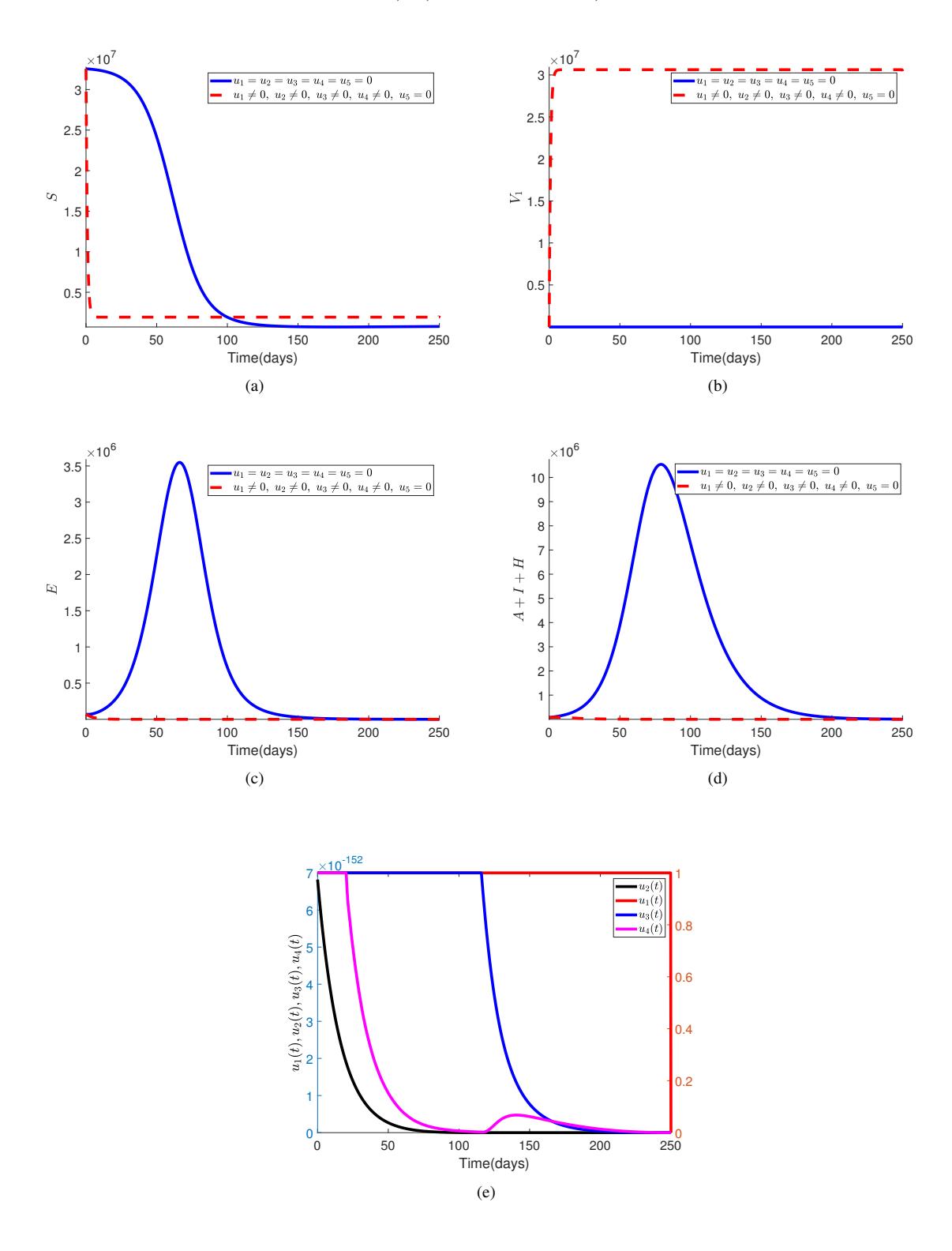
Figure 9: Effect of strategy B1 \((u_1(t), u_2(t), u_3(t), u_4(t))\) on the optimal control COVID-19 model (3).
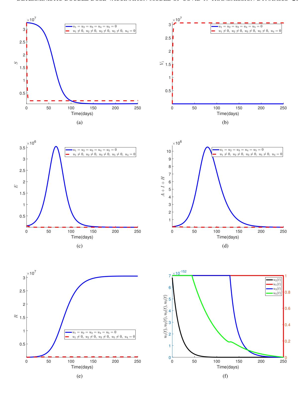
Figure 10: Effect of strategy B2 \((u_1(t), u_2(t), u_3(t), u_5(t))\) on the optimal control COVID-19 model (3).
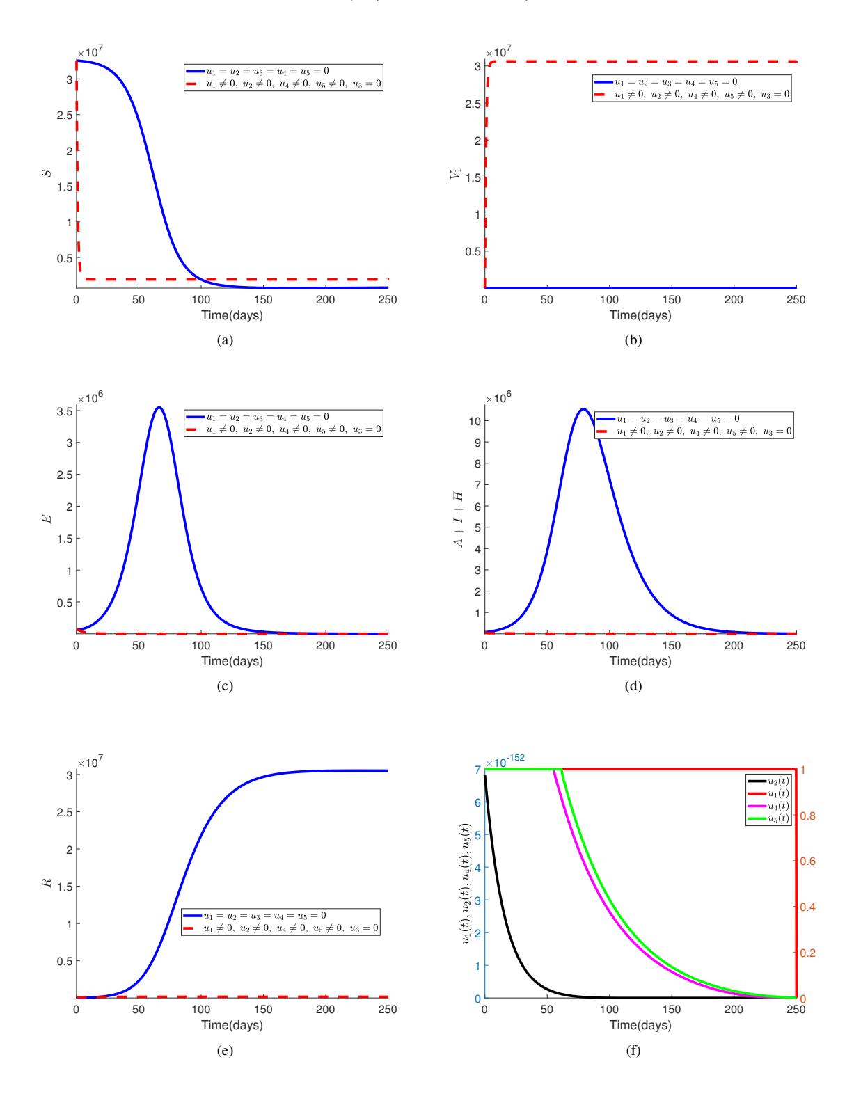
Figure 11: Effect of strategy B3 \((u_1(t), u_2(t), u_4(t), u_5(t))\) on the optimal control COVID-19 model (3).
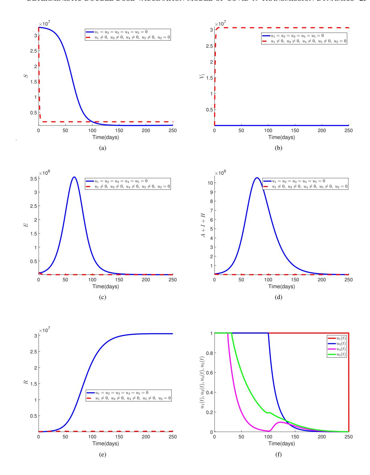
Figure 12: Effect of strategy B4 (u1(t), u3(t), u4(t), u5(t)) on the optimal control COVID-19 model (3).
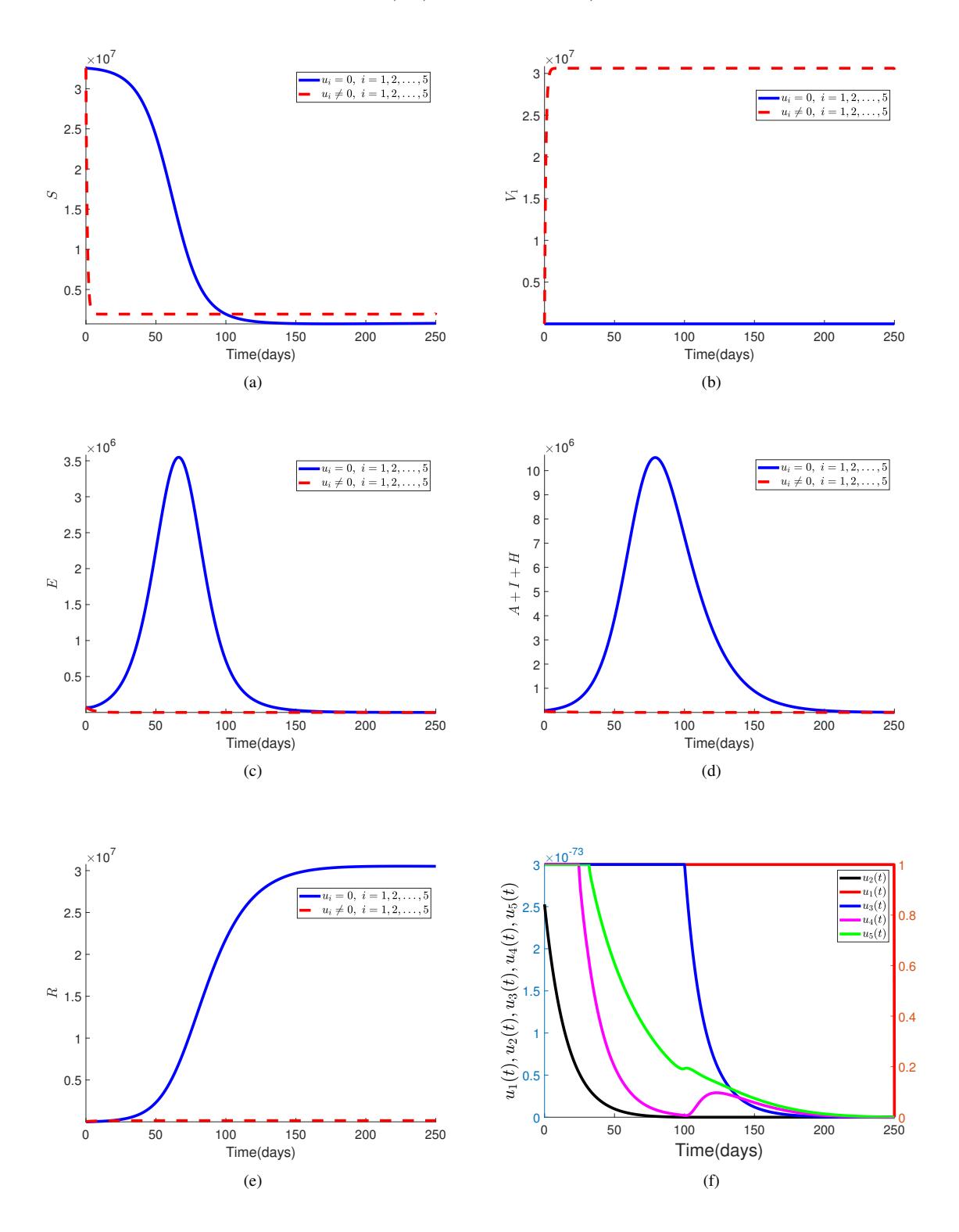
Figure 13: Effect of strategy C \((u_1(t), u_2(t), u_3(t), u_4(t), u_5(t))\) on the optimal control COVID-19 model (3).
3) Implementation of the quintuple intervention strategy in Group C: Figure 13 presents the combined impact of applying all control measures (first dose vaccination, second dose vaccination, personal protection, testing, and treatment) against COVID-19, aimed at minimizing the objective functional (4) in conjunction with the state system (3). By implementing these controls simultaneously, the trajectories demonstrate a significant reduction in the susceptible, exposed, infected, and recovered subpopulations, leading to the vanish of disease prevalence throughout the control implementation regime. The control profiles, as depicted in Figure 13(f), illustrate how each measure is optimized and sustained to achieve the desired outcome. The comprehensive application of first dose vaccination over the intervention period, continuous use of optimal second dose vaccination near its lower bound, and application of optimal personal protection, screening or testing and treatment controls maximally for 120, 30 and 50 days, respectively, before reducing gradually to their minimum levels of implementation at time Ft = 250 days yields numerous benefits in combating COVID-19. This approach provides a multifaceted defence against the virus, bolstering individual and population immunity through vaccinations, reducing transmission with personal protection measures, detecting and isolating cases promptly through testing, and ensuring appropriate medical care for infected individuals through treatment. The combination of these controls facilitates a rapid decline in COVID-19 cases, effectively curbing outbreaks and easing the burden on healthcare systems. Furthermore, the comprehensive strategy offers the potential for long-term disease control, potentially leading to the eradication or near-eradication of COVID-19 within the population, thus safeguarding public health and enhancing community well-being.
4.2. Cost-effectiveness analysis
It is necessary to choose the most cost-effective intervention strategy among the potential combinations of the five time-dependent controls taken into consideration in light of the simulation results for the optimal control problem as obtained in the immediate previous section. Two techniques – the average cost-effectiveness ratio (ACER) and the incremental cost-effectiveness ratio (ICER) in the sense of [30], [38] – are used to do this. In the first case, ACER is focused on a specific intervention strategy and compares the intervention to its baseline option. It is the proportion of the intervention's overall cost to the total number of infections it prevents. Thus, the mathematical calculation of ACER can be performed through the following formula:
\[ACER = \frac{\text{Total cost expended on a particular intervention}}{\text{Total cases of infection averted by the same intervention}}.\] (11)
According to this cost analysis approach, the control intervention strategy with the least ACER value among the list of alternative intervention strategies competing for the same available resources is the most costeffective [39].
Distinguishing between two alternative strategies that compete for the same resources, ICER is interested in comparing their costs and health outcomes. It represents the change in the costs of the two alternative strategies divided by the change in the total number of infections averted by using the two strategies. This can be simply put in mathematical form as
\[ICER = \frac{Change in the cost of interventions}{Change in the total number of infections averted}.\] (12)
It is not difficult to calculate the ACER and ICER values for the competing intervention strategies based on the formulae in (11) and (12) with the aid of the following explicit formulae extracted for the total cost produced by a particular intervention strategy and the total infection averted by the intervention strategy as derived from the objective functional (4):
\[\begin{split} &\text{Total cost} = \frac{1}{2} \int_0^{F_t} \sum_{i=1}^5 n_i u_i^2 dt, \\ &\text{Total infection averted} = \int_0^{F_t} \left(A + I + H\right) dt - \int_0^{F_t} \left(A_* + I_* + H_*\right) dt, \end{split}\] where A and A∗ are the total number of asymptomatic individuals without and with control strategy, respectively, I and I∗ are the total number of symptomatic individuals without and with control strategy, respectively, while H and H∗ are the total number of hospitalized individuals without and with control strategy, respectively.
1) Triple control intervention strategies: Here, the most cost-effective intervention strategy from the list of seven strategies in Group A is determined with the aid of ACER and ICER cost analysis methods. In Table 3, strategies Ai, where i = 1, 2, . . . , 7, in Group A are listed in an increasing order of the total infections prevented, along with the expenses associated with each. ACER for the seven strategies are calculated with the use of the formula in (11), and the results are as displayed in the 4th column of Table 3. Looking at the table, it is apparent that strategy A7 produces the least ACER value followed by strategy A2, strategy A3, strategy A6, strategy A4, strategy A1 and strategy A5. Therefore, strategy A7 is the most cost-effective strategy required for preventing and controlling the transmission and spread of COVID-19 in Group A according to ACER cost analysis approach.
Table 3: ACER for strategies A1 to A7 and ICER for the competing strategies A3 and A2.
| Strategy | Infection averted (×109 ) | Cost (×105 ) | ACER (×10−5 ) | ICER |
|---|---|---|---|---|
| A3: u1, u2, u5 | 2.600993 | 1.524192 | 5.860040 | 5.860039 × 10⁻⁵ |
| A2: u1, u2, u4 | 2.601023 | 1.426377 | 5.483909 | −0.326050 |
| A1: u1, u2, u3 | 2.601448 | 1.683036 | 6.469610 | − |
| A4: u1, u3, u4 | 2.603820 | 1.675688 | 6.435500 | − |
| A5: u1, u3, u5 | 2.603943 | 1.830538 | 7.029872 | − |
| A6: u1, u4, u5 | 2.608804 | 1.607632 | 6.162335 | − |
| A7: u3, u4, u5 | 2.609481 | 0.657714 | 2.520477 | − |
Furthermore, the fifth column of Table 3 shows the ICER for the alternative strategies A3 and A2, which are calculated based on the formula in (12) as follows:
ICER for strategy A3 = \[\frac{1.524192 \times 10^5}{2.600993 \times 10^9} = 5.860039 \times 10^{-5}\], ICER for strategy A2 = \(\frac{(1.426377 - 1.524192) \times 10^5}{(2.601023 - 2.600993) \times 10^9} = -0.326050\).
When the ICERs of strategies A3 and A2 are compared, it is apparent that the ICER for strategy A3 is higher than that of strategy A2. This simply indicates that strategy A3 is strongly dominated by strategy A2. As a consequence, strategy A3 is more expensive and less effective to implement. Thus, strategy A3 is removed from the list of competing strategies. By the same procedure, ICER is re-calculated for the competing strategies A2 and A1 using (12). Table 4 displays the results generated from the calculations.
Table 4: ICER for strategies A3 and A2.
| Strategy | Infection averted (×109 ) | Cost (×105 ) | ICER |
|---|---|---|---|
| A2: u1, u2, u4 | 2.601023 | 1.426377 | 5.483908 × 10⁻⁵ |
| A1: u1, u2, u3 | 2.601448 | 1.683036 | 6.039035 × 10⁻² |
| A4: u1, u3, u4 | 2.603820 | 1.675688 | − |
| A5: u1, u3, u5 | 2.603943 | 1.830538 | − |
| A6: u1, u4, u5 | 2.608804 | 1.607632 | − |
| A7: u3, u4, u5 | 2.609481 | 0.657714 | − |
A look at Table 4 shows that the ICER for strategy A2 is less than the ICER for strategy A1. This suggests that strategy A2 strongly dominates strategy A1, implying that strategy A2 is cheaper and more effective to implement when compared to strategy A1. Therefore, strategy A1 is discarded from the list of alternative strategies, while ICER is further re-calculated for strategy A2 competing with strategy A4. The computed results are summarized in Table 5.
From Table 5, comparison between the ICER for strategy A2 and strategy A4 reveals that the ICER for strategy A4 is greater than the ICER for strategy A2. This simply suggests that strategy A4 is strongly dominated by strategy A2. This means that strategy A4 is more expensive and less effective to implement compared to strategy A2. Hence, strategy A4 is discarded from the list of alternative intervention strategies that can be implement to curb COVID-19 transmission and spread in the community. Again, the ICER is
Table 5: ICER for strategies A2 and A4.
| Strategy | Infection averted (×109 ) | Cost (×105 ) | ICER |
|---|---|---|---|
| A2: u1, u2, u4 | 2.601023 | 1.426377 | 5.483908 × 10⁻⁵ |
| A4: u1, u3, u4 | 2.603820 | 1.675688 | 8.913514 × 10⁻³ |
| A5: u1, u3, u5 | 2.603943 | 1.830538 | − |
| A6: u1, u4, u5 | 2.608804 | 1.607632 | − |
| A7: u3, u4, u5 | 2.609481 | 0.657714 | − |
re-computed for the competing strategy A2 and strategy A5 using the explicit formula (12), and the results are shown in Table 6.
Table 6: ICER for strategies A2 and A5.
| Strategy | Infection averted (×109 ) | Cost (×105 ) | ICER |
|---|---|---|---|
| A2: u1, u2, u4 | 2.601023 | 1.426377 | 5.483908 × 10⁻⁵ |
| A5: u1, u3, u5 | 2.603943 | 1.830538 | 1.384113 × 10⁻² |
| A6: u1, u4, u5 | 2.608804 | 1.607632 | − |
| A7: u3, u4, u5 | 2.609481 | 0.657714 | − |
It is clear that the ICER for strategy A2 is less than the ICER for strategy A5 as shown in Table 6, following the comparison between the ICER value for strategy A2 and the ICER value for strategy A5. This suggests that strategy A2 is cheaper and more effective to implement when compared with strategy A5. Thus, it is economical to eliminate strategy A5 from the list of alternative strategies that can be implemented. Therefore, strategy A5 is discarded from further consideration while strategy A2 further competes with strategy A6. Using the explicit formula (12), the ICER values for strategies A2 and A6 are obtained. The results are presented in Table 7.
Table 7: ICER for strategies A2 and A6.
| Strategy | Infection averted (×109 ) | Cost (×105 ) | ICER |
|---|---|---|---|
| A2: u1, u2, u4 | 2.601023 | 1.426377 | 5.483908 × 10⁻⁵ |
| A6: u1, u4, u5 | 2.608804 | 1.607632 | 2.329456 × 10⁻³ |
| A7: u3, u4, u5 | 2.609481 | 0.657714 | − |
In Table 7, the comparison between strategy A2 and strategy A6 shows that ICER for strategy A6 is greater than ICER for strategy A2. This means that strategy A2 strongly dominates strategy A6, implying that strategy A6 is more costly and less effective to implement than strategy A2. As a consequence, strategy A6 is removed from the list of alternative interventions. At this juncture, ICER is re-computed for the remaining strategy A2 and strategy A7 competing for the same available resources using the formula in (12). Table 8 gives the summary of the ICER computation results.
Table 8: ICER for strategies A2 and A7.
| Strategy | Infection averted (×109 ) | Cost (×105 ) | ICER |
|---|---|---|---|
| A2: u1, u2, u4 | 2.601023 | 1.426377 | 5.483908 × 10⁻⁵ |
| A7: u3, u4, u5 | 2.609481 | 0.657714 | −9.088004 × 10⁻³ |
From Table 8, comparison between strategy A2 and strategy A7 shows that ICER for strategy A2 is greater than ICER for strategy A7. This simply suggests that strategy A7 strongly dominates strategy A2, which means that strategy A7 is less costly and more effective to implement than strategy A2. Consequently, strategy A2 is eliminated from the list of alternative strategies. Therefore, the most cost-effective strategy in Group
A according to ICER cost analysis method is strategy A7 (combination of personal protection, testing or screening and treatment). This validates the preceding findings of the ACER method.
2) Quadruple control intervention strategies: In this part, ACER and ICER cost analysis approaches are employed to establish the most cost-effective strategy in Group B. To do this, strategies B1, B2, B3 and B4 are composed in an increasing order of the total number of infections averted, along with the costs incurred on the implementation of each of the four intervention strategies as shown in Table 9. The Table also reflects the ACER values for all the strategies in Group B, which are calculated using the formula in (11).
Table 9: ACER for strategies B1 to B4 and ICER for the competing strategies B1 and B2.
| Strategy | Infection averted (×109 ) | Cost (×105 ) | ACER (×10−5 ) | ICER |
|---|---|---|---|---|
| B1: u1, u2, u3, u4 | 2.603820 | 1.675730 | 6.435660 | 6.435660 × 10⁻⁵ |
| B2: u1, u2, u3, u5 | 2.603943 | 1.830570 | 7.029992 | 1.258862 × 10⁻¹ |
| B3: u1, u2, u4, u5 | 2.608804 | 1.607698 | 6.162588 | − |
| B4: u1, u3, u4, u5 | 2.609482 | 1.759347 | 6.742134 | − |
From the fourth column of Table 9, it is seen that strategy B3 produces the least ACER value. The next strategy that produces the least ACER value is strategy B1, followed by strategy B4 and strategy B2. Therefore, strategy B3, which is the combination of first dose vaccination, second dose vaccination, testing or screening, and treatment, is the most cost-effective strategy in Group B based on the ACER cost analysis approach.
To reaffirm this result, ICER approach is employed. The ICER values for the competing strategies B1 and B2 are computed using (12), and are presented in the fifth column of Table 9. Following the comparison between strategy B1 and strategy B2 in Table 9, it is observed that the ICER value for strategy B1 is less than the ICER value for strategy B2. Thus, strategy B2 is strongly dominated by strategy B1. This means that strategy B2 is more costly and less effective to implement than strategy B1. Therefore, strategy B2 is eliminated from the list of competing intervention strategies, while strategy B1 is retained in the list. So, strategy B1 further competes with strategy B3. The ICER values for these competing strategies are obtained using the formula in (12), and the results are presented in Table 10.
Table 10: ICER for strategies B1 and B3.
| Strategy | Infection averted (×109 ) | Cost (×105 ) | ICER |
|---|---|---|---|
| B1: u1, u2, u3, u4 | 2.603820 | 1.675730 | 6.435660 × 10⁻⁵ |
| B3: u1, u2, u4, u5 | 2.608804 | 1.607698 | −1.365008 × 10⁻³ |
| B4: u1, u3, u4, u5 | 2.609482 | 1.759347 | − |
It is observed from Table 10 that the ICER for strategy B1 is greater than the ICER for strategy B3, suggesting that strategy B3 strongly dominates strategy B1. This means that strategy B3 is less costly and more effective to implement than strategy B1. As a result, strategy B1 is discared from the list of alternative strategies that can be implemented. Finally, strategy B3 further competes with strategy B4 for the available resources. Thus, the ICER values for the competing strategies are obtained using the explicit formula (12), and the results are displayed in Table 11.
Table 11: ICER for strategies B1 and B3.
| Strategy | Infection averted (×109 ) | Cost (×105 ) | ICER |
|---|---|---|---|
| B3: u1, u2, u4, u5 | 2.608804 | 1.607698 | 6.162586 × 10⁻⁵ |
| B4: u1, u3, u4, u5 | 2.609482 | 1.759347 | 2.236711 × 10⁻² |
Comparing strategy B3 and strategy B4, it is seen from Table 11 that the ICER for strategy B4 is greater than the ICER for strategy B3. This simply suggests that strategy B4 is strongly dominated by strategy
B3, meaning that strategy B4 is more costly and less effective compared with strategy B3. Thus, strategy B4 is discarded from the list of alternative strategies. Therefore, strategy B3 (combination of the first dose vaccination, second dose vaccination, testing or screening and treatment) is the most cost-effective strategy in Group B according to ICER cost analysis method. This result aligns with the result of ACER cost analysis approach obtained earlier.
3) Quintuple control intervention strategy: Table 12 presents the total infection averted by, the total cost expended on and the ACER for strategy C. Since the only intervention strategy in Group C is the combination of all the five time-varying control variables \(u_i(t)\), \(i=1,2,\ldots,5\), the ACER and ICER values for the strategy are both \(6.742107 \times 10^{-5}\). As a consequence, there is nothing to compare in this situation.
Table 12: ACER for strategies C.
| Strategy | Infection averted | Cost | ACER |
|---|---|---|---|
| C: \(u_1, u_2, u_3, u_4, u_5\) | \(2.609482 \times 10^9\) | \(1.759340 \times 10^5\) | \[6.742107 \times 10^{-5}\] |
4) Identification of the overall most cost-effective strategy: In this part, the overall most cost-effective strategy from the list of most cost-effective strategies in Groups A (strategy A7), B (strategy B3) and C (strategy C) is further identified based on both the ACER and ICER cost analysis approaches.
The ACER values of strategies A7, B3 and C are displayed in Figure 14. It is seen from Figure 14 that strategy A7 has the least ACER value, this is followed by strategy B3, while strategy C has the highest ACER value. Thus, according to ACER cost analysis approach, the overall most cost-effective strategy among all the various control combination strategies considered in this paper is strategy A7, which is the combination of personal protection, testing (or screening) and treatment. From Figure 15, it is clear that strategy A7, which involves the least number of control interventions when compared with the other two strategies (B3 and C), averts almost the same number of infections in the population (approximately to the nearest billion). In fact, the strategy averts more number of infections than strategy B3 as shown in Table 13. Furthermore, Figure 16 clearly shows that strategy A7 produces the least cost of control implementation to reach the optimal prevention and control of COVID-19 in the population as illustrated in Figure 8.
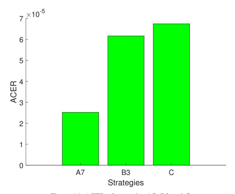
Figure 14: ACER of strategies A7, B3 and C.
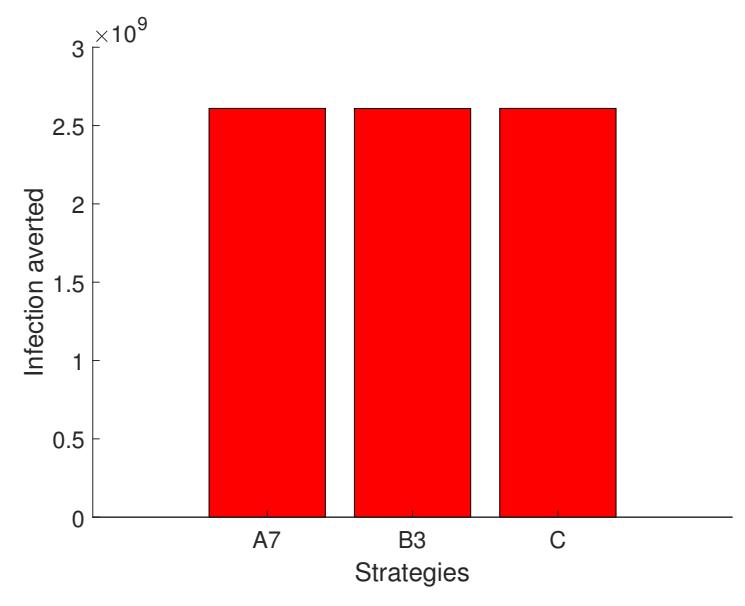
Figure 15: Total infection averted with the implementation of intervention strategies A7, B3 and C.
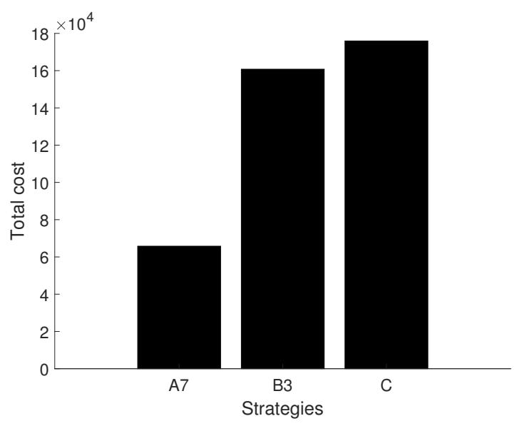
Figure 16: Total cost incurred on control strategies A7, B3 and C implementation.
In Table 13, strategies A7, B3 and C, which are identified as the most cost-effective strategies in Group A, Group B and Group C, respectively, are arranged in an increasing order of the total number of infections averted along with the total cost incurred on the strategies. Using the explicit formula in (12), the calculated ICER values for the competing strategies B3 and A7 are as appeared in the fourth column of Table 13. By comparison between strategies B3 and A7, it is shown that the ICER of strategy B3 is greater than the ICER of strategy A7. The economic implication of this is that strategy B3 is more expensive and less effective than
Table 13: ICER for strategies B3 and A7.
| Strategy | Infection averted (×109 ) | Cost (×105 ) | ICER |
|---|---|---|---|
| B3: u1, u2, u4, u5 | 2.608804 | 1.607698 | 6.162586 × 10⁻⁵ |
| A7: u3, u4, u5 | 2.609481 | 0.657714 | −1.403227 × 10⁻¹ |
| C: u1, u2, u3, u4, u5 | 2.609482 | 1.759340 | − |
strategy A7. As a result, strategy B3 is eliminated from the list of competing strategies. Further analysis is conducted on the remaining competing strategies A7 and C by recalculating ICER using formula (12). The outcomes of the calculations are dsiplayed in Table 14.
Table 14: ICER for strategies A7 and C.
| Strategy | Infection averted (×109 ) | Cost (×105 ) | ICER |
|---|---|---|---|
| A7: u3, u4, u5 | 2.609481 | 0.657714 | 2.520477 × 10⁻⁵ |
| C: u1, u2, u3, u4, u5 | 2.609482 | 1.759340 | 1.101626 × 10² |
Comparison between strategy A7 and strategy C reveals that the ICER of strategy A7 is less than the ICER of strategy C. Thus, strategy A7 strongly dominates strategy C, implying that strategy A7 is less expensive and more effective to implement when compared with strategy C. Thus, strategy C is removed from the list of alternative strategies. Therefore, strategy A7 in Group A is the overall most cost-effective strategy that can be implemented to effectively prevent and control the transmission dynamics and spread of COVID-19 in the population. This result reaffirms the previous result obtained through ACER method.
5. CONCLUSION
This study expands upon an existing deterministic COVID-19 model, transitioning it from a non-optimal control approach to an optimal control framework. The objective is to gain insights into the most effective and economical strategies for mitigating COVID-19 transmission across different optimal control scenarios. The enhanced optimal control COVID-19 model incorporates five time-dependent control variables accounting for first dose vaccination, second dose vaccination, personal precautionary measures, testing, and treatment. The optimal control model in this paper gives a more realistic optimal control framework for COVID-19 compared to the existing similar works (e.g., see [18], [21], [22], [23], [24], [25]), by taking into account these five control interventions which allow for the economic evaluation of different meaningful combination strategies involving the utilized of at least three of the five control interventions. Thorough analysis of the model is carried out to establish the existence and characterize the optimal control quintuple. This is achieved by applying optimal control theory along with the Pontryagin's maximum principle. The efficiency of each control intervention is quantified within various control combination strategies including the utilizing of at least three control interventions, which are stratified into three distinct groups (namely, triple control interventions, quadruple control interventions and quintuple control intervention), to identify the strategies that best mitigate COVID-19 spread in the population through numerical simulations. In each of the three groups, ACER and ICER cost analysis methods are employed to determine the most cost-effective strategy. In Group A, it is discovered from the results of both cost analysis methods that the most cost-effective intervention strategy is the combination of personal protection, testing or screening and treatment. Both methods agree that combination of first dose vaccination, second dose vaccination, testing or screening and treatment is the most cost-effective strategy in Group B. For robustness, the overall most cost-effective intervention strategy to prevent and manage the dynamics of COVID-19 transmission in the community is a strategy that combines personal protection, testing or screening and treatment based on two cost analysis methods. These findings suggest that the implementation of the Group C strategy involving the combination of all the five time-dependent control interventions is recommend to curb the transmission and community spread of COVID-19 when the resources are readily available. Meanwhile, implementation of the overall most cost-effective intervention strategy which is made up of personal protection, testing or screening and treatment is strongly recommended to effectively curb the community spread of the pandemic when the resource allocation is limited.
In this paper, the numerical implementation of the optimal control model is carried out based on theoretical (assumed) values of the weight constants related to the objective functional (4). As such, the study can be strengthened by also calibrating the model to the data case of COVID-19 control cost in Malaysia in a future work.
ACKNOWLEDGEMENTS
The handling editor and anonymous reviewers are sincerely appreciated by the authors for their insightful and helpful feedback, which considerably enhanced the presentation of the original manuscript.