

1. Introduction
Researchers from several scientific domains such as biology, physics, chemistry, nanotechnology, and others have recently become interested in the issue of nanoparticles, as it is a challenging impact for the present real world problems. Nanoparticles have many applications but they can sometimes harm living species from humans to marine plankton system. Zinc oxide nanoparticles are known to be cytotoxic to human immune cells, as reported by Kokate et al. [1]. According to the scientific representatives' report on consumer safety, nanomaterials were also discovered in sunscreens and cosmetics [2]. The implications for human health are still unknown, though. In their study, Oszlánczi et al. [3] discovered that diesel nanoparticles can damage mice's cardiovascular systems. On the other hand, Miglietta et al. [4] looked at the eco-toxicological consequences of different kinds of nanoparticles on the marine environment. Various forms of nanoparticles' having toxicity to aquatic species such as plants, fungi, algae, invertebrates and fish which has been described in the recent last two decades [5], [6], [7], [8], [9].
Nanomaterials are found naturally as the simulated products by combustion reactions. Some are produced specifically through biochemical engineering process to perform a specialised function due to availability of nanoparticles in a simulated environment and in chemical reaction resultants. A set of particles with different sizes between 1 and 100 nm are referred to as nanoparticles and they are distinguished from other types of particles by certain physicochemical characteristics such as surface area, surface charge, degree of aggregation,
<sup>1</sup>Department of Interdisciplinary Sciences, National Institute of Food Technology Entrepreneurship and Management, Kundli, Haryana 131028, India
<sup>2</sup>Department of Mathematics, School of Advanced Sciences, Vellore Institute of Technology, Vellore 632014, India <sup>3</sup>Department of Mathematics, Aliah University, Kolkata 700156, India <sup>4</sup>Mathematics Dicipline, Khulna University, Khulna 9208, Bangladesh
*Corresponding author
Received August \(26^{th}\), 2023, Revised January \(9^{th}\), 2024 (first), Revised May \(31^{st}\), 2024 (second), Accepted for publication June \(30^{th}\), 2024. Copyright ©2024 Published by Indonesian Biomathematical Society, e-ISSN: 2549-2896, DOI:10.5614/cbms.2024.7.1.8
particle shape and surface coating. Due to extensive use by many different industries, nanoparticles have either been intentionally or accidentally released into the aquatic environment.
Researchers are investigating the various properties like origins, behaviours, toxicological impacts of NPs due to the interference in aquatic systems due to excessive usage [29]. In an effort to promote the sustainable use of these novel materials, a number of recent studies have considered the ecological effects of nanoparticles, including fate, transport, and toxicity [30], [31], [32]. Nonetheless, the majority of these investigations have focused on how nanoparticles affect human health.
Nanoparticles are found in a variety of items like drug delivery, cancer therapy, cosmetics, sun screens, clothing, paints, lithium-ion batteries, fertilizer, processed foods and so on which can end up in the aquatic environment. This can happen during manufacturing, usage or disposal either directly or indirectly. Furthermore, nanoparticles can be produced by natural occurrences such as forest fires, volcanic eruptions, weathering and the production of clay minerals, erosion caused by wind and water, and dust storms in desert environments [10]. Before sinking into saltwater, these wildly diverse sized nanoparticles have the ability to traverse thousands of kilometers and hang suspended in midair for several days [10]. Since released nanoparticles eventually dissolve in seawater, it can be important to observe how they behave there to determine any potential risks to marine life. The way that nanoparticles behave and disperse in aquatic environments largely dictate how they interact with marine life, and surface speciation is often associated with risk [11]. The internalization of nanoparticles and/or their attachment to phytoplankton cells have the potential to inhibit the growth of several phytoplankton species in maritime environments.
While natural nanoparticles (NPs) including clays, minerals, and products generated from microorganisms have been used for ages, artificial nanoparticles are the outcome of deliberate design and engineering [31]. Different transformation processes that control the effects of ENPs on ecological systems after their discharge into the aquatic environment are possible [33]. Controlling and defining the toxicity of engineered nanoparticles requires an understanding of these transition processes. However, a number of factors related to the nanoparticles themselves, the environment, and the model organism under examination affect how hazardous the particles are [34].
The aquatic environment is given a lot of attention since it serves as the primary entry and dispersal point for nanoparticles into other natural resources, acting as a "link" in the process [35]. Depending on the kind of nanoparticle, the concentration in surface water can range from less than ng per liter to ug per liter. In surface water, TiO2 is the most concentrated at 2.2 grams per liter, followed by Ag NP at 1.5 mg per liter, according to the European Union.
Natural nanoparticles have been interacting with many living things for millions of years, as was already mentioned, throughout the environment. Contrarily, produced NPs creep into our daily life and keep growing without our knowledge. The design of manufactured NPs incorporates certain surface chemistries and features that offer them distinct toxicological and physico-chemical characteristics in comparison to natural ones [36].
Additionally, studies were conducted on the toxicity of silver, copper, aluminum, nickel, and cobalt nanoparticles in zebra fish, daphnids, and algae species [12], [13], [14]. When exposed to normal amounts of ultraviolet radiation, titanium dioxide nanoparticles have been found to have a significant harmful effect on marine phytoplankton. Miller et al. [13] investigated the toxicity of nanoparticles in terms of slowing population growth in an experimental setting. They utilized four common phytoplankton species—Isochrysis galbana, Thalassiosira pseudonana, Dunaliella tertiolecta, and Skeletonema costatum—to represent the three main groupings of diatoms, green algae, and prymnesiophytes. Studies employed two levels of UV radiation (exposed and blocked) and five levels of TiO2 concentration 0, 1, 3, 5, and 7 mg. In the UV-exposed condition, three of the four species had a notable decline in population growth. They came to the conclusion that nanoparticles can significantly slow the population expansion of the first three species mentioned when they are exposed to ultraviolet light. They believe that the intake of nanoparticles is one factor impacting the proliferation of algae. Miao et al. [12] showed that Ag-ENs can be taken up and held inside algal cells, where they can cause harm. Thus, internalizing nanoparticles may be a different strategy for regulating the growth of algae. The freshwater alga Ochromonas Danica was significantly poisoned by treatment with increased concentrations of Ag-EN. At Ag-EN concentrations of 139.1, 185.4, and 278.1 M (elemental molarity of Ag), cell growth was reduced by 18.8, 40.3, and 100 percent respectively. They also discovered that marine phytoplankton is harmed by zinc oxide nanoparticles. Furthermore, Suwannee River fulvic acid promoted the internalization of CuO nanoparticles, which was shown to occur in complete algal cells via high-resolution transmission electron microscopy [28].
Moreover, water-dispersed nanoparticles can readily attach to the cell membranes of phytoplankton, preventing their growth. The most important processes that affect the destiny of nanoparticles in aquatic settings include agglomeration, aggregation, dissolution, and chemical interactions, such as oxidation or reduction, ligand exchange, and the development of new solid phases [16], [17], [18], [19]. Recently, Castro-Bugallo et al. [8] conducted an experiment that demonstrated the harmful effects of zinc oxide and yttrium oxide on marine microalgae. Furthermore, whether stated in terms of cell counts and biomass, they discovered that population growth rate was the variable most vulnerable to the acutely harmful impacts of both nanoparticles. Citrate-coated silver nanoparticles are more dangerous to cultures in their early stages, according to research by Stevenson et al. [7] on the freshwater alga Chlamydomonas reinhardtii at different phases of batch culture growth. The effects of citrate-coated silver nanoparticles on phytoplankton development and their relationships with the availability of phosphorus (P) were investigated by Das et al. [9]. The researchers found that maximal phytoplankton growth rates are limited by 11–85 percentage by citrate-coated silver nanoparticles. They hypothesised that the destiny and toxicity of citrate-coated silver nanoparticles in aquatic environments would depend on the level of phosphorus contamination. Because of the harm that nanoparticles can do to ecological systems, it is quite concerning when they are released into an aquatic environment [20].
The impacts of nanoparticles on individuals and/or communities, as well as interactions with phytoplankton, have been demonstrated in the majority of experimental studies; nonetheless, the impact of nanoparticles on the aquatic food chain remains poorly understood. Investigating the relationship between nanoparticles and phytoplankton as well as the potential effects on the aquatic food chain is therefore fascinating. To the best of our knowledge, this is the first attempt to use mathematical models to explain the connection between phytoplankton and nanoparticles. In this research, we begin modeling aspects of such dynamics by concentrating on a phytoplankton-zooplankton system affected by nanoparticles.
Phytoplankton is the main producer in both freshwater and marine systems. It gives higher trophic levels in the food chain (either herbivore or omnivore) energy and nutrients. It has been demonstrated that primary producers in the aquatic food chain are negatively impacted by nanoparticles. It goes without saying that in-depth investigation is needed by both theorists and experimentalists in studies concerning the interaction of phytoplankton with nanoparticles. In this research, we propose that the intrinsic growth rate of phytoplankton populations is lowered by nanoparticles. There is an inverse relationship between the concentration of nanoparticles in the aquatic environment and the rate of phytoplankton growth. We employ a basic phytoplankton-zooplankton model and incorporate a component that represents phytoplankton-nanoparticle interactions in order to study the effect of nanoparticles on plankton dynamics. We will have a better understanding of how nanoparticles impact plankton dynamics thanks to the model analysis. It is important to remember that our research is focused on the reduction of phytoplankton development caused by nanoparticles, not zooplankton. The main goal of the study is to examine how nanoparticles affect the dynamics of a simple phytoplankton-zooplankton system.
Below is a breakdown of the task. The mathematical model and the boundedness of its solutions are presented in the following section. For each equilibrium site, a local stability analysis is conducted in Section 3. Additionally, we discover how "NPs" affect equilibrium densities and stability standards for various functional responses. In Section 4, we investigate the existence, direction, and stability of Hopf-bifurcation around interior equilibriums. In Section 5, numerical simulations are carried out. Finally, we evaluate and draw inferences from our results.
2. FORMULATION OF MATHEMATICAL MODEL
We first employ a basic predator-prey model, in which the populations of phytoplankton and zooplankton represent the populations of prey and predators, respectively, to study the effects of nanoparticles on a phytoplankton-zooplankton system. The mathematical model is expressed using a set of ordinary differential equations, as the following example illustrates.
\[\frac{dP}{dt} = \frac{rP}{1+\beta\beta_1 N_{\alpha}P} \left( 1 - \frac{P}{K} \right) - \frac{cPZ}{\gamma P^2 + b} \frac{dZ}{dt} = \frac{dcPZ}{\gamma P^2 + b} - \mu Z\] (1)
Here P is the prey density of phytoplankton and Z is the predator density of zooplankton at time t. In the absence of Z, P grows logistically with intrinsic growth rate r and carrying capacity K. Z predates
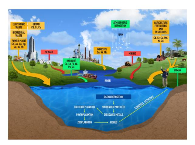
Figure 1: Pictorial representation of the model.
P following the Haldane functional response (Reference, year) with predation rate c, saturation constant b which are scaling the impact of the predator interference and food weighting factor. The parameter d is the efficiency of transforming prey intake into new predator, and \(\mu\) is the natural death rate of the predator. Here we chose the Monod Haldane functional response as this type of functional response was first introduced by Haldane [23] in enzymology. It was then used by Andrews [24] as saturate uptake function. For detailed discussion in this direction, interested readers may consult the book by Kot [25]. Sugie et.al. [26] proposed a simplified Monod Haldane functional response of the form \(f(p) = \frac{p}{\gamma P^2 + b}\). In this case, b is also a positive parameter, and it represents the inhibitory effect's inverse measure.
Moreover, we believe that when nanoparticles in the aquatic system come into contact with phytoplankton, they stick to the cell membrane of the phytoplankton and occasionally even enter the cell. Free nanoparticles are removed from the aquatic system by attachment of nanoparticles in phytoplankton cells. We include the consumption of nanoparticles by phytoplankton in the model system after we have mathematically modeled the uptake of free viruses by bacteria [27] (Figure-1). We extend the preceding model in the presence of nanoparticles as follows, taking into account the assumptions previously stated:
\[\frac{dP}{dt} = \frac{rP}{1+\beta\beta_1 N_{\alpha}P} \left( 1 - \frac{P}{K} \right) - \frac{cPZ}{\gamma P^2 + b} \frac{dZ}{dt} = \frac{dcPZ}{\gamma P^2 + b} - \mu Z \frac{dN_{\alpha}}{dt} = A - N_{\alpha}P - eN_{\alpha}\] (2)
All parameters are expected to be positive in this case. It's worth noting that, in the absence of nanoparticles, Model (2) becomes Model (1).
3. MODEL ANALYSIS
3.1. Boundedness
Theorem 3.1. All solutions of system (2) in \(\mathbb{R}^3_+\) are "uniformly bounded".
Proof: From the system (2), we have \(\frac{dN_{\alpha}}{dt} \leq A - d_1N_{\alpha}\) i.e. \(\frac{dN_{\alpha}}{dt} - d_1N_{\alpha} \leq A\). Therefore, \(0 < N_{\alpha}(t) \leq e^{-d_1t} \left(N_{\alpha}(0) - \frac{A}{d_1}\right) + \frac{A}{d_1}\). As \(t \to \infty\), \(N_{\alpha}(t) \to A/d_1\), since \(\sup N_{\alpha}(t) = A/d_1\). Let W = dP + Z and let us calculate the derivative of W, we obtain
\[\begin{split} \frac{dW}{dt} & \leq dr P \left(1 - \frac{P}{K}\right) - \mu Z, \\ \frac{dW}{dt} & + \eta W \leq P \left(dr + \eta d - dr \frac{P}{K}\right) + (\eta - \mu) \, Z, \end{split}\]
\[\frac{dW}{dt} + \eta W \le m.\]
Here \(\eta < d_1\), \(m = \frac{r_2 K_1 (r_1 + \eta)^2}{4r_1}\); Therefore, \(0 < W(t) \le e^{-\eta t} \left(W(0) - \frac{1}{\eta}\right) + \frac{1}{\eta}\) As \(t \to \infty, W(t) \to m/\eta\). i.e. \(W(t) \le m/\eta\), since sup \(W(t) = m/d_1\). System (2) is therefore restricted above. This suggests that over an extended period of time, none of the interacting species grow exponentially. Because resources are limited, the population of any species is finite.
3.2. Existence of Equilibrium Points
The system has four possible steady states as \(E_0\) (0,0,0), \(E_1\) \((0,Z^\phi,N^\phi_\alpha)\), \(E_2\) \((P^l,0,N^l_\alpha)\), \(E_3\) \((P^m,Z^m,0)\), \(E_4\) \((P^*,Z^*,N^*_\alpha)\) where \(Z^\phi=0\); \(N^\phi_\alpha=\frac{A}{e}\); \(P^l=K\); \(Z^l=0\); \(N^l_\alpha=\frac{A}{K-e}\);
\[\begin{split} P^m &= \frac{dc \pm \sqrt{(dc)^2 - 4\mu^2 b \gamma}}{2\mu \gamma}; Z^m = (\gamma P^m + b) \left(1 - \frac{P^m}{K}\right); \\ P^* &= \frac{dc \pm \sqrt{(dc)^2 - 4\mu^2 b \gamma}}{2\mu \gamma}; Z^* = \frac{\left(\gamma^2 P^* + b \gamma\right)}{c\left(1 + \beta \beta_1 N_\alpha^* P^*\right)} \left(1 - \frac{P^*}{K}\right); N_\alpha^* = \frac{A}{P^* - e}. \end{split}\]
For \(P^*\) to be positive, we must have, \(dc > 2\mu\sqrt{b\gamma}\) and for \(N^*_{\alpha}\) to be positive, we must have \(b > \frac{dce}{\mu} - \gamma e^2\). for \(Z^*\) to be positive, we must have \(K > P^*\).
3.3. Local Stability Analysis
In this part, we analyze the linear stability of Model (2). The linearization method can be used to examine the local behavior of a complex nonlinear system. Typically, we linearize the system around each steady state point, slightly disturb it, and then observe whether the system converges to that steady state point again or to a different one. Through the use of local stability analysis, qualitative behavior of complex dynamical systems can be better understood.
Lemma 3.2. The system (2) around \(E_4(P^*, Z^*, N_\alpha^*)\) is locally asymptotically stable if the root of the characteristic equation \(\lambda^3 + A_1\lambda^2 + A_2\lambda + A_3 = 0\) of the 'Jacobian matrix' \(J(E^*)\) satisfies 'Routh-Hurwitz characteristic equation \(\lambda^{\circ} + A_{1}\lambda^{-} + A_{2}\lambda + A_{3} = 0\), criteria' i.e., \(A_{1} > 0, A_{3} > 0, A_{1}A_{2} - A_{3} > 0\), where \(J(E^{*}) = \begin{bmatrix} J_{11} - \lambda & J_{12} & J_{13} \\ J_{21} & J_{22} - \lambda & J_{23} \\ J_{31} & J_{32} & J_{33} - \lambda \end{bmatrix}.\)
\[J(E^*) = \begin{bmatrix} J_{11} - \lambda & J_{12} & J_{13} \\ J_{21} & J_{22} - \lambda & J_{23} \\ J_{31} & J_{32} & J_{33} - \lambda \end{bmatrix}\]
\(J_{11} = \frac{r}{(1+\beta\beta_1N_{\alpha}P)^2} - \frac{r(2P+\beta\beta_1N_{\alpha}P)}{(1+\beta\beta_1N_{\alpha}P)^2} - \frac{cZ(b-\gamma P^2)}{(\gamma P^2+b)^2}; \ J_{12} = \frac{\mu}{d}; \ J_{13} = 0; \ J_{21} = \frac{\mu\left(b-\gamma P^{*^2}\right)}{P^*}; \ J_{22} = 0; \ J_{23} = 0; \ J_{31} = -N_{\alpha}^*; \ J_{32} = 0; \ J_{33} = -P^* - e \ \text{and} \ A_1 = P^* - J_{11} + e; \ A_2 = -J_{11}P^* - J_{11}e - \frac{J_{21}\mu}{d}; \ A_3 = -\frac{\mu J_{21}(P^*+e)}{d}.\)For \(A_1 > 0, A_3 > 0, A_1A_2 - A_3 > 0\), we must have \(P^* + e > J_{11}\) and \(P^* > \sqrt{b/\gamma}\).
3.4. Global Stability Analysis
In this section, we investigated the global stability behavior of the system (2) at the interior equilibrium \(E_4(P^*, Z^*, N_\alpha^*)\) by using the Lyapunov stability theorem.
Theorem 3.3. The system (2) is globally asymptotically stable about \(E_4(P^*, Z^*, N_{\alpha}^*)\)
Proof: Let us consider the Lyapunov function
\[V(P, Z, N_{\alpha}) = \left(P - P^* - \log\left(\frac{P}{P^*}\right)\right) + l_1\left(Z - Z^* - \log\left(\frac{Z}{Z^*}\right)\right)\]\[+l_2\left(N_{\alpha} - N_{\alpha}^* - \log\left(\frac{N_{\alpha}}{N_{\alpha}^*}\right)\right).\]
Differentiating \(V(P, Z, N_{\alpha})\) with respect to 't' we get,
\[\frac{dV}{dt} = \left(P - P^*\right) \frac{dP}{dt} + l_1 \left(Z - Z^*\right) \frac{dZ}{dt} + l_2 \left(N_\alpha - N_\alpha^*\right) \frac{dN_\alpha}{dt},\] where \(l_1, l_2\) are positive constants.
\[\frac{dV}{dt} = (P - P^*) c \left[ \frac{P^* Z^*}{\gamma P^{*2} + b} - \frac{PZ}{\gamma P^2 + b} \right] + l_1 (Z - Z^*) z \left[ \frac{dcP}{\gamma P^2 + b} - \frac{dcP^*}{\gamma P^{*2} + b} \right] + l_2 (N_{\alpha} - N_{\alpha}^*) [N_{\alpha} P^* + N_{\alpha}^* e - N_{\alpha} P - N_{\alpha} e].\]
By choosing \(l_1 = \frac{1}{e}\); \(l_2 = \frac{\left(\gamma P^2 + b\right)\left(\gamma P^{*2} + b\right)}{dc(b - \gamma P P^*)}\),
\[\frac{dV}{dt} \le -\frac{c\gamma\beta\beta_1 N_{\alpha} (P - P^*)^2}{K (1 + \beta\beta_1 N_{\alpha} P) (1 + \beta\beta_1 N_{\alpha} P^*)} + \frac{dc (b - \gamma P P^*)}{(\gamma P^2 + b) (\gamma P^{*2} + b)} \left[ \frac{(P - P^*)^2}{2} + \frac{(Z - Z^*)^2}{2} \right] - \frac{N_{\alpha}}{e} \left[ \frac{(N_{\alpha} - N_{\alpha}^*)^2}{2} + \frac{(P - P^*)^2}{2} \right] - (N_{\alpha} - N_{\alpha}^*)^2,\]
which implies that \(\frac{dV}{dt} < 0\). Therefore, the system (2) is globally asymptotically stable about \(E_4\left(P^*,Z^*,N_{\alpha}^*\right)\).
3.5. Impact of Nanomaterial for Different Functional Responses
Three varieties of functional responses like Holling Type I, Holling Type II, Monod Haldane are commonly utilized in the literature to represent the phytoplankton-zooplankton system with their biological underpinnings [21], [22]. We also investigate the influence of the various functional responses on the system's stability behavior. We compared the model (2) to the Holling type I, Holling type II, Beddington, and Monod Haldane functional responses in order to illustrate this point. Rather of providing the explicit model analysis for the Beddington functional responses, Holling type I and Holling type II, we provide the stability requirements of these three types of responses. Citational responses are displayed in Table 1.
Table 1: The stability conditions for several equilibriums of Model 2 with different functional responses.
| Steady states | Holling Type-I | Holling Type-II | Monod Haldane |
|---|---|---|---|
| \(E_0\) \(E_1\) | Unstable | Unstable | Unstable |
| \(E_1\) | Unstable | Unstable | Unstable |
| \(E_2\) | Stable if \(dck < \mu\) | Stable if \(dck < \mu(b+K)\) | Stable if \(r/(1 + \beta \beta_1 N_{\alpha} P)^2 < e\) |
| \(E_4\) | Stable | Stable | Stable if \(P^* > \sqrt{b/\gamma}\) |
The detailed model analysis for the Holling type I and Holling type II functional responses is absent from Table 1, which instead shows the stability criteria for the three distinct types of functional responses. The phytoplankton-zooplankton free state \(E_0(0,0,0)\) and another state \(E_1(0,Z^\phi,N^\phi_\alpha)\) are always unstable for all forms of functional responses, as seen in Table 1. The preceding table also includes the stability conditions for interior equilibriums. We chose two critical factors such as interaction rate of Nanoparticle-Phytoplankton and natural depletion rate of Nano particles and fixed the remaining parameters because depicting the role of the functional responses with regard to the entire parameter space is unfeasible. Then, using Table 1, we adjust these two important factors and see the model's stability behavior of the system (2). Section 10 has a full numerical analysis with illustrations.
| Type of Interaction | In the absence of Nanoparticles | In the presence of Nanoparticles |
|---|---|---|
| Holling Type-I | \[P^* = \frac{\mu}{dc};\] | \[P^* = \frac{\mu}{dc};\] |
| \[P^* = \frac{\mu}{dc};\] \[Z^* = \frac{\gamma(1 - \frac{\mu}{Kdc})}{2}\] | \[P^* = \frac{\mu}{dc};\] \[N^*_{\alpha} = \frac{A}{\beta P^* + e};\] | |
| 2 — c | \[Z^* = \frac{\gamma \left(1 - \frac{P^*}{K}\right)}{c(1 + \beta \beta_1 N_{\alpha}^* P^*)}\] \[P^* - \frac{\mu b}{c}.\] | |
| \(Z' = \frac{1}{c(1+\beta\beta_1 N_{\alpha}^* P^*)}\) | ||
| Holling Type-II | \[P^* = \frac{\mu b}{dc - \mu \gamma};\] | \[P^* = \frac{\mu b}{dc - \mu};\] \[N^*_{\alpha} = \frac{A}{\beta P^* + e};\] |
| \[P^* = \frac{\mu b}{dc - \mu \gamma};\] \[Z^* = \frac{\gamma dP^* \left(1 - \frac{P^*}{K}\right)}{2}\] | \(N_{\alpha}^* = \frac{A}{\beta P^* + e};\) | |
| \(Z^* = \frac{1}{\mu}\) | \[Z^* = \frac{\gamma(b+P^*)\left(1-\frac{P^*}{K}\right)}{c(1+\beta\beta_1N_{\alpha}^*P^*)}\] | |
| \(c(1+\beta\beta_1N_{\alpha}^*P^*)\) | ||
| Monod Haldane | \[P^m = \frac{dc \pm \sqrt{(dc)^2 - 4\mu^2 b\gamma}}{2\mu\gamma};\] | \[P^* = \frac{dc \pm \sqrt{(dc)^2 - 4\mu^2 b\gamma}}{2\mu\gamma};\] |
| \[P^{m} = \frac{dc \pm \sqrt{(dc)^{2} - 4\mu^{2}b\gamma}}{2\mu\gamma};\] \[Z^{m} = (\gamma P^{m} + b)\left(1 - \frac{P^{m}}{K}\right)\] | \[Z^* = \frac{\left(\gamma^2 P^{*+b\gamma}\right)}{c\left(1+\beta\beta_1 N_{\alpha}^* P^*\right)} \left(1 - \frac{P^*}{K}\right);\] \[N_{\alpha}^* = \frac{A}{P^* - e}\] | |
| \[N_{\alpha}^* = \frac{A}{P^* - e}\] |
Table 2: The interior equilibrium points of Model 2 with different functional responses when nanoparticles are present or absent.
3.6. Hopf Bifurcation Analysis
Theorem 3.4. At a critical contact rate, the system (2) experiences Hopf bifurcation around the positive equilibrium. The existence of \(\beta = \beta^*\) such that Hopf bifurcation occurs is a necessary and sufficient condition (i) \(H(\beta^*) \equiv A_1(\beta^*)A_2(\beta^*) - A_3(\beta^*) = 0\), (ii) \(\frac{d}{d\beta} [\text{Real part of } \lambda(\beta)]_{\beta=\beta^*} \neq 0\), where \(\lambda\) is a characteristic equation root corresponding to the inner steady state.
Proof: For \(\beta=\beta^*\), we can write the characteristic equation \(\lambda^3+A_1\lambda^2+A_2\lambda+A_3=0\) as \((\lambda^2+A_2)(\lambda+A_1)=0\), which has three roots \(\lambda_1=i\sqrt{A_2},\ \lambda_2=-i\sqrt{A_2},\lambda_3=-A_1\). The roots for all \(\beta\) are, in general, of the form \(\lambda_1(\beta)=\mu_1(\beta)+i\mu_2(\beta),\ \lambda_2(\beta)=\mu_1(\beta)-i\mu_2(\beta),\ \lambda_3(\beta)=-A_1\). Now we'll test the condition of transversality \(\frac{d}{d\beta}\) [Real part of \(\lambda\) (\(\beta\))]\(_{\beta=\beta^*}\neq 0;\ j=1,2\). We may calculate the derivative by substituting \(\lambda_j(\beta)=\mu_1(\beta)+i\mu_2(\beta)\) into the characteristic equation. \(M(\beta)\mu_1^{'}(\beta)-N(\beta)\mu_2^{'}(\beta)+S(\beta)=0; \ (\beta)\mu_1^{'}(\beta)+M(\beta)\mu_2^{'}(\beta)+R(\beta)=0, \ \text{where} \ M(\beta)=3\mu_1^{2}(\beta)+2A_1(\beta)\mu_1(\beta)+A_2(\beta)-3\mu_2^{2}(\beta), \ N(\beta)=6\mu_1(\beta)\mu_2(\beta)+2A_1(\beta)\mu_2(\beta).\)
\[S(\beta) = \mu_1^2(\beta) A_1^{'}(\beta) + A_2^{'}(\beta) \mu_1(\beta) + A_3^{'}(\beta) - A_1^{'}(\beta) \mu_2^2(\beta),\]
\[R(\beta) = 2\mu_1(\beta) \mu_2(\beta) A_1^{'}(\beta) + A_2^{'}(\beta) \mu_2(\beta).\]
Taking note of this, \(\mu_1(\beta^*) = 0\), \(\mu_2(\beta^*) = \sqrt{A_2\beta^*}\), \(M(\beta^*) = -2A_2(\beta^*)\), \(N(\beta^*) = -2A_1(\beta^*)\sqrt{A_2\beta^*}\), \(S(\beta^*) = A_1^{'}(\beta^*) - A_1^{'}(\beta^*)A_2(\beta^*)\), \(R(\beta^*) = A_2^{'}(\beta)\sqrt{A_2\beta^*}\),
\[\begin{split} \frac{d}{d\beta} \left[ \text{Real part of } \lambda\left(\beta\right) \right]_{\beta=\beta^*} &= \frac{N(\beta^*)R(\beta^*) + M(\beta^*)S(\beta^*)}{M(\beta^*)^2 + N(\beta^*)^2} \\ &= -\frac{2A_1(\beta^*)\sqrt{A_2(\beta^*)} \times A_2^{'}(\beta^*)\sqrt{A_2(\beta^*)} + (-2A_2(\beta^*)) \left[A_3(\beta^*) - A_1^{'}(\beta^*)A_2(\beta^*)\right]}{(-2A_2(\beta^*))^2 + \left(2A_1(\beta^*)\sqrt{A_2(\beta^*)}\right)^2} \\ &= -\frac{A_1(\beta^*)A_2^{'}(\beta^*) - A_3^{'}(\beta^*) + A_1^{'}(\beta^*)A_2(\beta^*)}{2\left[A_1(\beta^*) + A_2(\beta^*)\right]^2}, \end{split}\]
provided, \(A_1(\beta^*)A_2'(\beta^*) - A_3'(\beta^*) + A_1'(\beta^*)A_2(\beta^*) \neq 0\) and \(\lambda_3(\beta^*) = -A_1(\beta^*) \neq 0\). As a result, the transversality conditions are met. This means that at \(\beta = \beta^*\), a Hopf bifurcation occurs. Then, the theorem is established.
3.7. Effect of Nanoparticles in Marine Ecological System
The influence of nanoparticles on the aquatic food chain is especially noteworthy, as evidenced by the relationship between phytoplankton and zooplankton. As a result, the crucial parameter \(\beta\) is the contact rate between phytoplankton and Nanoparticles, i.e. More Nanoparticles will affect the sea food chain if the contact rate is higher. To identify the only mechanism after adding nanoparticles to the system, we study the shift in the equilibrium density of prey and predator. The impacts of nanoparticles on the equilibrium densities of zooplankton and phytoplankton for different functional responses are compared in this section. To investigate the interaction rate with and without nanoparticles, we calculated the phytoplankton and zooplankton equilibrium densities (Table 2). When the Holling Type I functional response is activated, the equilibrium density of phytoplankton stays constant whereas the equilibrium density of zooplankton decreases as it grows. Regarding the Holling Type II functional response, a comparable outcome is achieved. Therefore, the prey population density stays constant for Holling type I and II functional responses; this can be thought of as zooplankton population top-down control on phytoplankton. However, the Z* and P* equilibrium densities decrease as for the Monod Haldane functional response. It should be noted that although while experimental data indicates that phytoplankton development is restricted and cell density is decreased by nanoparticles, if zooplankton emerges earlier than phytoplankton as a result of Holling Type I, II functional responses, then nanoparticles have no influence on P* equilibrium densities. In theory, we believe that a more accurate model of the phytoplankton-zooplankton system in the presence of hazardous nanoparticles is the Monod Haldane functional response. In section 10, a graphical illustration of the influence of Nanoparticles on phytoplankton and zooplankton equilibrium densities is shown to make it clearer.
4. NUMERICAL SIMULATIONS
In order to investigate the dynamics of the model, we perform numerical simulations of the model, with the following parameter values.
Example-1: \[r = 2\]; \(K = 20\); \(c = 0.8\); \(\mu = 0.08\); \(d = 0.33\); \(\gamma = 1\); \(b = 8\); \(A = 5\); \(e = 0.05\); \(\beta = 0.12\); \(\beta_1 = 0.8\).
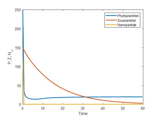
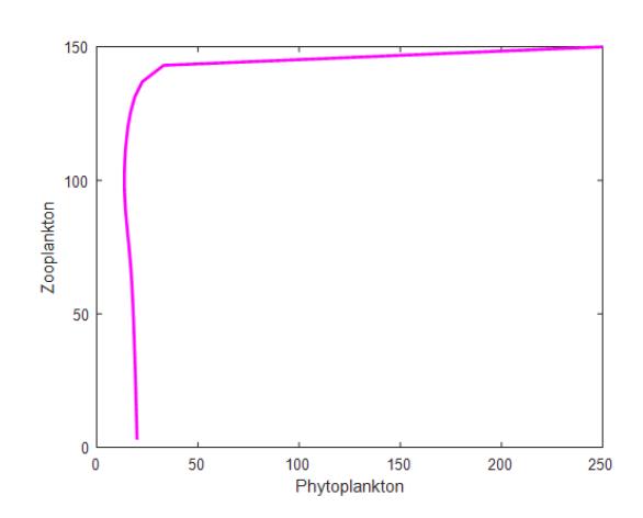
Figure 2: The time series evaluation of Phytoplankton, Zooplankton and Nanoparticle densities.
Figure 3: The variation in Zooplankton with respect to Phytoplankton.
Figure 2 represents the time series plot of Phytoplankton, Zooplankton and Nanoparticles with the values of Example-1 which are appropriate for the model. Figure 3 represents the Variation projection of the Zooplankton against the Phytoplankton species for the values of Example-1 which says clearly as Zooplankton density increases along with the increase in Phytoplankton and justified the model which is considered.
Figure 4 represents the Variation projection of the Phytoplankton against the Nanoparticles with the values of Example-1 which clearly says that Phytoplankton slightly increases with the addition of nanoparticles to the aquatic ecosystem. Figure 5 represents the variation projection of the Zooplankton against the Nanoparticles with the values of Example-1 which clearly says that Zooplankton slightly increases with the addition of nanoparticles to the aquatic ecosystem.
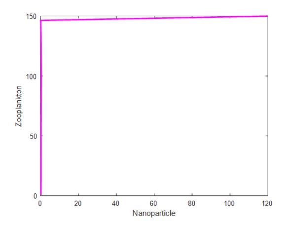
Figure 4: The variation in Zooplankton with respect to Nanoparticles.
Figure 5: The variation in Phytoplankton with respect to Nanoparticles.
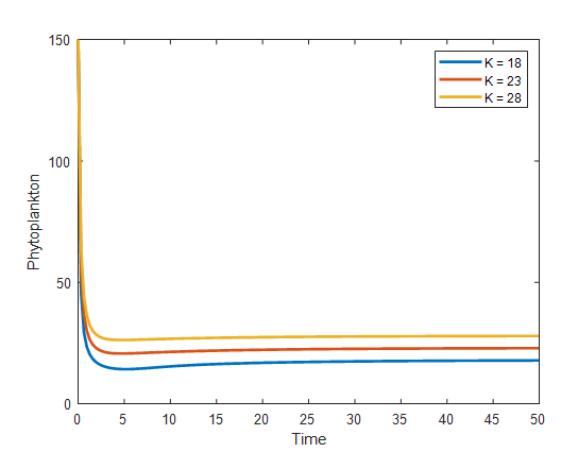
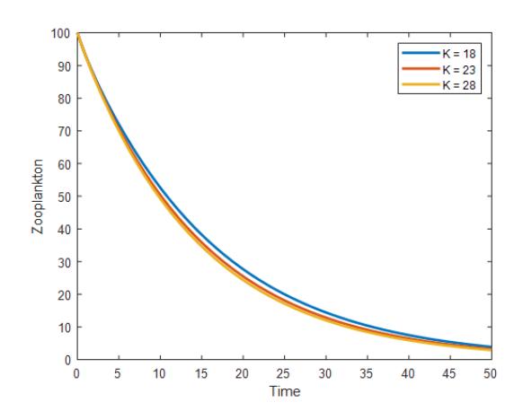
Figure 6: The time series evalutaion of Phytoplankton with the variations in K.
Figure 7: The time series evaluation of Zooplankton with the variations in K.
Figure 6 represents time series plot of Phytoplankton variated projections along with the variation in K values with the attributes of Example-1. The projections of Phytoplankton for various values of K shows that as K increases correspondingly Phytoplankton density also increases. Figure 7 represents time series plot of Zooplankton variated projections along with the variation in K values with the attributes of Example-1. The projections of Zooplankton for various values of K shows that as K increases correspondingly Zooplankton density not varies remarkably almost negligible and the projections are almost emerging. Very closely observes than the slight variation says that Zooplankton decreases for the increasing values of K.
Figure 8 represents time series plot of Nanoparticle variated projections along with the variation in K values with the attributes of Example-1. The projections of Nanoparticle for various values of K shows that as K increases correspondingly Nanoparticle doesn't show any variation. Variation in the projections of Nanoparticle is almost negligible.
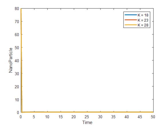
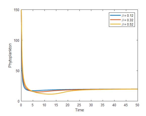
Figure 8: The variation in Nanoparticles with the variation in K.
Figure 9: The variation in Phytoplankton with the variation in β.
Figure 9 represents time series plot of Phytoplankton variated projections along with the variation in β values with the attributes of Example-1. The projections of Phytoplankton for various values of β shows that as β increases, correspondingly Phytoplankton density decreases. The variation in the projections of Phytoplankton is very less and stating that as β increases, Phytoplankton density slightly decreases.
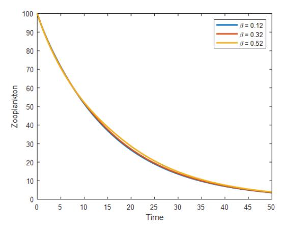

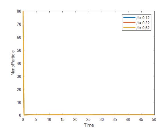
Figure 11: The variation in Nanoparticles with the variation in β
Figure 10 represents time series plot of Zooplankton variated projections along with the variation in β values with the attributes of Example-1. The projections of Zooplankton for various values of β shows that as β increases correspondingly Zooplankton density increases. The variation in the projections of Zooplankton is very less and emerging one with the other and stating that as β increases Zooplankton density slightly increases.
Figure 11 represents time series plot of Nanoparticle variated projections along with the variation in β values with the attributes of Example-1. The projections of Nanoparticle for various values of β shows that as β increases correspondingly Nano particle doesn't show any variation. Variation in the projections of Nano particle is almost negligible.
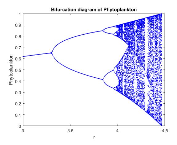
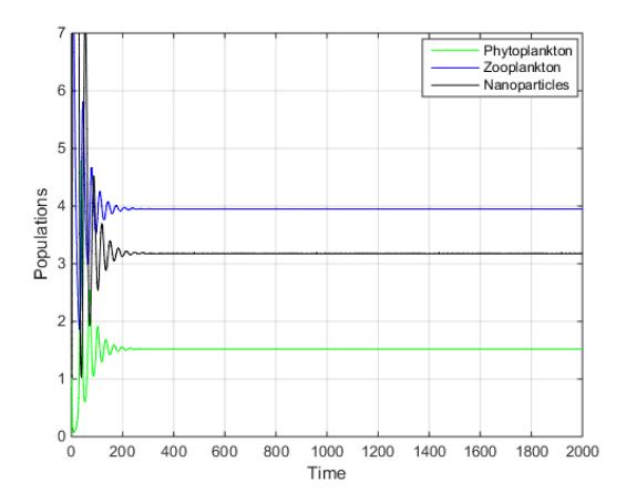
Figure 12: Bifurcation diagram of Phytoplankton with respect to intrinsic growth rate r
Figure 13: The time series solution of the system variables
From figure 12, it is observed that Phytoplankton highly bifurcates between the range 3.3 to 4.5. Later on slowly it attains stability. Initially Phytoplankton bifurcates at (3.3, 0.65284) and further bifurcates at two points (3.845, 0.849045) and (3.845, 0.414239). Again, for further phytoplankton bifurcates very slowly at four points (3.965, 0.881837), (3.96, 0.813696), (3.96, 0.502149) and (3.96, 0.33273). As intrinsic growth rate increases, phytoplankton bifurcates well in the presence of Nanoparticle also. Here Nanoparticle plays a constructive role in the system dynamics and its stability. We can say that Nanoparticle benefits the system indirectly towards stability and density of the population.
Figure 13 ensures that the system variables are persisting in the long run and converging to the equilibrium point (1.52, 3.95, 3.18) for the same parameter values: r = 2; K = 20; c = 0.8; µ = 0.08; d = 0.33; γ = 0.01; b = 5; A = 5; e = 0.05; β = 0.5; β1 = 0.8.
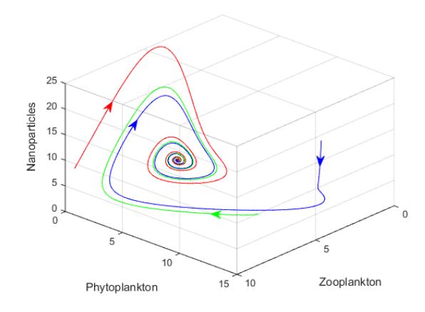
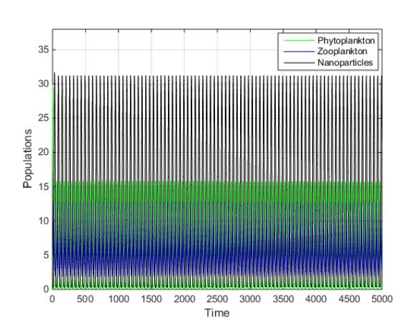
Figure 14: The phase portrait from different initial points converging to the interior equilibrium point.
Figure 15: The periodic solutions of the system variables arising from Hopf-bifurcation.
Figure 14 ensures that the interior equilibrium point (1.52, 3.95, 3.18) is globally asymptotically stable. Parameter values remain same as of Figure 13. Figure 15 represents the periodic solutions of the system variables. Parameter values remain same as of Figure 13 except γ = 0.1. Therefore, γ is a very sensible
parameter for the proposed system. Figure 16 shows the existence of a stable closed orbit corresponding to the periodic solution.
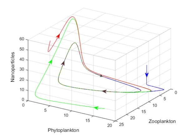
Figure 16: The existence of a stable limit cycle plotted from different initial points.
5. DISCUSSION AND CONCLUDING REMARKS
Particularly in the last ten years, nanoparticles have become an essential component of modern life. It is utilized "everywhere" in our daily lives, including in the cosmetics and electronics industries. As a result, nanoparticles disrupt the environment and raise a number of concerns, especially about their path and consequences. Numerous published studies examined the types, characteristics, applications, and consequences of nanoparticles. But only a few of them concentrated on the Nano particle effect on aquatic eco systems which consists of Phytoplankton and Zooplankton.
Finally, we would like to point out that the findings of this work are based on the notion that nanoparticle attachment in phytoplankton cells inhibits phytoplankton growth. Furthermore, we discovered that the equilibrium density of zooplankton and phytoplankton populations is lowered by interactions between phytoplankton and nanoparticles. Furthermore, when the rate of contact between nanoparticles and phytoplankton rises, Hopf-bifurcation may cause limit cycle oscillations in the phytoplankton-zooplankton system. For a range of functional responses, the existence and local stability of the system's equilibriums have been investigated within a specific parameter range. To the best of our knowledge, this is the first mathematical model that looks into how nanoparticles impact the interactions between phytoplankton and zooplankton. It involves phytoplankton, zooplankton, and nanoparticles.
We also looked into the impact of various functional responses on population dynamics. Our theoretical findings show that the Monod Haldane functional response is better suited to capturing such dynamics than the Holling type I, and Holling type II, functional responses. Our results also suggest that the stable coexistence of plankton populations depends on the rate at which nanoparticles are removed from the aquatic environment.
We carried out a comprehensive numerical study to support and clarify our findings. Our current work's analytical and numerical results indicate that nanoparticles may have significant dynamical effects in a simple phytoplankton-zooplankton model. Given the implications of our findings, empirical study to assess these theories is always needed. The growth of zooplankton is delayed when it consumes phytoplankton caused by nanoparticles. The dynamics of higher trophic levels may be impacted by this growth slowdown. Although the dynamics of the models will be intricate, they might have some fascinating features. We will deal with these matters in the future.
ACKNOWLEDGEMENT
We sincerely thank the Department of Mathematics, School of Advanced Sciences, Vellore Institute of Technology, Vellore, India, and the Department of Interdisciplinary Sciences at NIFTEM Knowledge Centre, Kundli, India, for their cooperation.
Declaration: The authors have no competing or conflict of interests to declare that are relevant to the content of this article.
Data availability: No data was used for the research described in the article.