

1. INTRODUCTION
Respiratory infection from virus is constant threat to society as it causes epidemic many times over past years [1]. In the end of year 2019, a viral respiratory infection, called Coronavirus Disease 2019 (COVID-19) was identified with higher reproduction rate and officially labeled as global pandemic [2]. Due to its impact on global economy, understanding of the infection dynamics become very crucial for future mitigation and prevention strategies.
In mathematics and statistics, many research have developed and studied techniques to gain insights or understanding of the condition, forecast future situations, or analyze the dynamics to prepare some measures, actions, or policies. One simple yet effective way to analyze the disease transmission is considering infection number as a time series, which allows statistical techniques such as ARIMA (Autoregressive Integrated Moving Average) to be effectively applied [3]. Recent popular method which uses deep learning approach such as Recurrent Neural Network (RNN), can also be implemented to predict the number of disease infections [4], [5], [6]. Apart from probabilistic approach, a more deterministic method using dynamical system can be used to simulate disease life-cycle within a population [7]. SIR (Susceptible-Infected-Recovered) model, as one of extensively used dynamical system in epidemiology, has been studied in various aspects of COVID-19 pandemic [8], [9], [10], [11]. The modified version of SIR, such as SEIR (Susceptible-Exposed-Infected-Recovered) model, is also used in the case of COVID-19 [12], [13].
In spite of its many advantages, SIR model depends on the assumptions used to formulate the governing equations of the system. In contrast, data-driven paradigm enables a construction of a mathematical model based on available data. This data A data-driven technique called SINDy (Sparse Identification of Nonlinear Dynamics) method has been developed to discover governing equations of dynamical system using data by regularized linear regression [14]. This kind of method is a mixing between mathematical techniques of differential equation with machine learning, where we can identify various governing physical models based on data and can modify using some additional techniques like using inductive bias [15], time-delay [16], or universal linear embedding [17].
This method has been developed and modified to various kind of mathematical model and problems, such as parametric PDE (partial differential equation) [18], boundary value problems [19], control system [20], [21], [22], hybrid dynamical system [23], discrete field [24], chaos forecasting [25], [26], Green's function
[27], and many others. SINDy also has been used in wide range of applications since then, including fluid dynamics [28], [29] and epidemiology [30].
The SINDy method is a data-driven technique that combines sparsity-promoting techniques and machine learning with nonlinear dynamical systems to discover governing equations from noisy measurement data. It assumes that there are only a few important terms that govern the dynamics, resulting in parsimonious models that balance accuracy with model complexity to avoid overfitting. This approach has been successfully applied to a wide range of problems, including linear and nonlinear oscillators, chaotic systems, and fluid dynamics [14].
The SINDy method has been applied to model and predict the transmission dynamics of COVID-19. For example, proposed a SINDy-LM modeling method that effectively balances model complexity and prediction accuracy [31]. They used the SINDy method to discover the nonlinear functional relationship between the dynamic terms in the model based on observation data of the COVID-19 epidemic. The obtained model was then optimized using the Levenberg-Marquardt algorithm to improve accuracy [31]. This approach has been used to review the epidemic situation in different countries and predict the evolution of the epidemic. The SINDy method can also be applied to analyze the dynamics of the COVID-19 pandemic by comparing and observing the parameters obtained [32].
Other studies have also explored the use of machine learning methods, such as neural networks and support vector machines, for predicting the spread of COVID-19 [33]. However, the SINDy method offers unique advantages in terms of interpretability and model complexity. It allows for the discovery of the underlying governing equations, providing insights into the fundamental dynamic relationships that drive the spread of the virus [14]. This can help researchers and policymakers better understand the mechanisms of transmission and develop more effective control strategies.
In this paper, we use SINDy to analyze the dynamics of the COVID-19 transmission in Indonesia during two different peak periods corresponding to different variants, Delta and Omicron. Complete SIR model with additional deceased groups (SIRD model) will be used. Data-constructed model may lose explainability as a trade-off with the accuracy. In that case, we also analyze the comparison of the dynamics in the terms of representation of some parameters obtained for explainability of the model.
2. MODEL FORMULATION
2.1. Compartmental model
The target of this study is to obtain and analyze compartmental model of COVID-19 infection based on data available. Compartmental model is a mathematical approach to describe a population dynamics by dividing the population in different groups/compartments. In epidemiology, the simplest form of this model is known as SIR model, where the population is divided to susceptible, infected, and recovered groups. The model itself is a system of first-order ordinary differential equation which govern how the number of people in each compartment changes over time. In general form, the SIR model can take following form
\[\frac{dS(t)}{dt} = f_1(S(t), I(t), R(t)), \frac{dI(t)}{dt} = f_2(S(t), I(t), R(t)), \frac{dR(t)}{dt} = f_3(S(t), I(t), R(t)),\] (1)
where S, I, and R, are number of people in respective compartment in a given time t. and fi for i = 1, 2, 3 are the functions that define the dynamics of the compartments. One characteristic of compartmental model is that it must satisfy S(t) + I(t) + R(t) = N(t), where N(t) represents total number of populations. This characteristic is satisfied if only birth rate and death rate of the populations are assumed to be small so it can be ignored. In the case of this paper, we only observe a short period of time that birth rate can be neglected. On the other hand, death values will be regarded as another compartment. The compartment itself can be added or modified depends on the assumption used in developing the model. For example, in the case where vaccination affect the spreading of the disease, new compartment V shall be added and gives SIRV model.
In the case of this study, we set the deceased individuals as a new compartment and symbolize it with D, giving the SIRD model.
SIR model has many variations based on the case it governs. The standard form only involves one non-linear term, i.e. the interaction between the susceptible and the infected. Usually, one use a set of assumptions to formulate the functions \(f_i\) and describe the dynamics from it. The purpose of this paper is to do the opposite. Given a set of real data, we want to predict the functions \(f_i\) by fitting the dynamics resulted from it.
2.2. Data processing
In this study, we use model with 4 compartments, i.e. susceptible (S), infected (I), recovered (R), and deceased (D). Other compartment that can be used in context of COVID-19 are vaccinated, second-susceptibility, and second-infection. Second-susceptibility and second-infection are different compartments than original susceptible and infected to accommodate the possibilities of getting re-infected after recovery. However, due to lack of available data, we exclude these three compartments even thought it may affect the whole dynamics. We want to see how the compartments affects the dynamics of each other differently during Delta and Omicron peak period.
We use data obtained independently by Our World in Data platform which contains original 3 features, i.e. susceptible, infected, and deceased [34]. For the recovery data, we use official data from government. Initially, we compile the data from the first identification of COVID-19 infection in Indonesia, March 2020, to the end of Omicron peak period, i.e. May 2022, which comprise of 781 datapoints. Because dealing with data containing large scale of values, such as population, may cause computational overflow, we take the normalized version of each compartment with respect to total population.
As susceptible group is relatively dominant compared to other groups, especially in the sense of total population of Indonesia, the number gap may cause overfitting in the regression process. We apply specific transformation to susceptible compartment to make sure it stays in roughly the same scale with other compartments. After that, standard normalization transformation using mean and standard deviation is applied to all compartments to obtain data with zero mean. As for the target variable, the gradients, we use numerical differentiation with time interval 0.1 day to obtain the derivatives of each compartment.
2.3. Sparse identification of nonlinear dynamics
The components and parameters within the system are typically predetermined based on a set of assumptions that form the foundation of the model's development. These assumptions are intended to be confirmed later using real-world data. However, an alternative approach is possible through the use of SINDy. By utilizing available data, we can construct a model that closely aligns with the data through the application of optimization techniques. This methodology allows us to effectively capture additional terms, particularly those that contribute significantly to the system's dynamics, including the nonlinear elements.
In general, if we encapsulate the four variables that characterize each compartment (namely, S, I, R, and D) into a vector represented as \(\vec{x}\), the general objective is to perform regression on the subsequent linear system
\[\frac{d\vec{x}}{dt} \approx \mathbf{W} \cdot \mathcal{P}_n(\vec{x}),\tag{2}\] where \(\mathcal{P}_n\) is a vector of n-th order monomial basis formed by \(\vec{x}\) and \(\mathbf{W}\) is the matrix of corresponding parameters. We can choose n arbitrarily depending on how many order of polynomial we want to consider in the dynamics. Ideally, all of the monomial basis will be use to search all possible polynomial that fit the data. We want that the model can capture every possible relations between the variables in the presence of the data. For example, elements of \(\mathcal{P}_2(\vec{x})\) are \(S^2\), \(I^2\), \(R^2\), \(D^2\), SI, SR, SD, IR, ID, and RD. Some relations, such as the one interacted with D variable, may gives little sense because the deceased individuals don't make contact with other compartment members. Nevertheless, there are many possible explanations in the relation that we can interpret beyond standard assumption of SIR model, such as psychological effect from the size of other compartments. For instance, the large number of recovered individual can induce positive effect on the infected ones, giving them more capability to be recovered. Although we have to minimize assumptions, to stimulate the appearance of interaction between compartment in the dynamics and to avoid model tendency to exploit easier deduction, we exclude all self-interaction terms (such as power terms \(S^2\)).
From a dataset comprising four distinct groups, we generate supplementary attributes that represent secondorder polynomial elements. If we exclude the intragroup interactions, this results in an extra set of six attributes. In the presence of these intragroup interactions, we would have an additional four attributes. Each of these newly created attributes is then treated as input for a linear regression model, with the derivatives of each group serving as the corresponding output.
Applying a conventional regression technique to the aforementioned linear equation could potentially result in a matrix W populated entirely with non-zero coefficients. However, it might not be desirable to establish a compartmental model in which each compartment is intricately linked to every other term and interaction. In order to attain a set of sparse coefficients, we employ an \(L_1\)-penalty as a form of regularization, known as LASSO (Least Absolute Shrinkage and Selection Operator) regression. We also employ \(L_2\) penalty, or Ridge regularization, to later analyze the effect of regularization to the total performance of the regression model. The combination of LASSO and Ridge is also commonly known as elastic net regularization [35]. The optimization procedure can be formulated as following.
\[\min_{\vec{w}_i} \left( \left\| \frac{dx_i}{dt} - \vec{w}_i \cdot \mathcal{P}_2(\vec{x}) \right\|_2^2 + \lambda_2 \|\vec{w}_i\|_2^2 + \lambda_1 \|\vec{w}_i\|_1 \right), \tag{3}\] for each i, where \(\lambda_1\) and \(\lambda_2\) is a parameter that represents the strength of the LASSO and Ridge regularization, respectively. In our case, \(x_i\) are S, I, R, and D, respectively for i = 1, 2, 3, 4.
2.4. Model analysis
In the context of regression, our objective is to anticipate the fluctuations (derivatives) within each compartment, taking into account the current population within each compartment and their interactions. The model is trained to fit the gradient of the compartment population given some combination of compartments. However, even thought the gradient is the one we regress as the target feature during model training, it is not the final intended output. Our primary concern lies in evaluating the compartmental model's ability to forecast compartmental quantities over a specific time span, based on initial data. Moreover, the model parameters after training itself is the one we need to analyze the learned system of SIRD model. To achieve this, a numerical integration employing the fourth-order Runge-Kutta method must be applied to the resulting model. We assess the mean squared error between the calculated infection values and the actual data. This error is additional metrics to evaluate the final model besides the mean squared error obtained during training and validation between the predicted and the true gradient. The overarching methodology described above can be visualized in a diagram, depicted in Figure 1.
3. RESULTS AND DISCUSSION
3.1. Data observation
The number of infected people over the time were fluctuating due to many external factors such as people's behavior, government regulation, economic condition, etc. These fluctuations imply that the parameters of the model are changing over time. However, we recognize that the shape of the dynamics are similar during the peak of two major variants of Delta and Omicron. We take the Delta period to start at June 3rd of 2021 and end at October 1st of 2021. On the other hand, we take the Omicron period to start at January \(15^{th}\) of 2022 and end at April \(19^{th}\) of 2022. The official date of each variant infection in Indonesia may differ with the date taken in this paper because officials marked the beginning of spreading of a variant as the first infection detected. In this paper however, we mark the beginning as the time where the number of infection increases significantly due to the variants.
We can see the dynamics in Figure 2. Because later we will also use the gradient data of each compartment, we also plot it in the figure. In a more detailed profile, we also plot in a closer look each period in Figure 3. It is shown how the shape of the dynamics are similar between Delta and Omicron period. These similarities indicate that the dynamical system governing them should have similar form, which we will investigate further in the next sections.
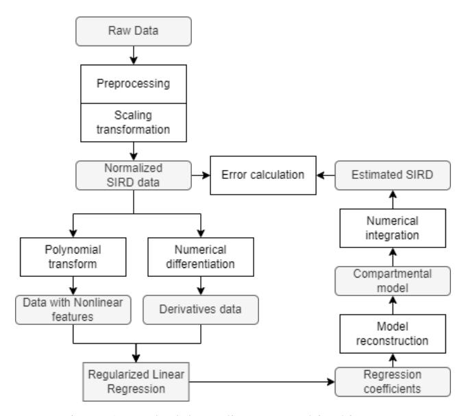
Figure 1: Methodology diagram used in this paper.
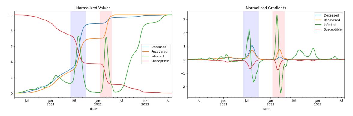
Figure 2: The profile of normalized compartmentalized population and its gradients. The light blue area represents Delta period and light red area represents Omicron period.
3.2. Model selection
We first select the best model by tuning the regularization strength used in the training. Because bias and self-interaction terms tends to reduce performance and also has quite low interpretability [32], in the model selection, we use directly second order polynomial consisting only single variable and interaction between different variables terms, which gives total 10 features as the only neurons of the model where the parameters are to be learned. SINDy model does not have complexities and hyperparameters to be tuned because the model itself is just a simple regressor. What we can tune instead, is the regularization added in the optimization process. Even thought SINDy require heavily to nonzero LASSO regularization, we also try to observe the effect of L2 penalty, or called Ridge regularization. The strength values of both L1 and L2 penalties are tuned in 1000 epochs with a stopper mechanism to break the iteration if the model is not learning significantly.
We trained the model in combination of two different values of L1, i.e. 0.01 and 0.05, and three different values of L2, i.e. 0, 0.01, and 0.05. We don't set L1 to 0 because LASSO regularization is necessary in
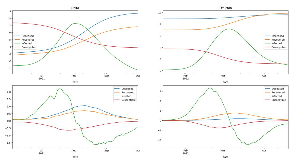
Figure 3: The close-up profile of normalized compartmentalized population and its gradients in two peak periods of variant Delta and Omicron.
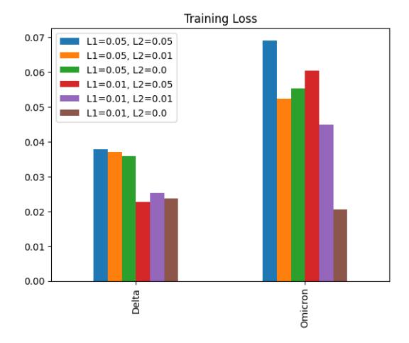
Figure 4: Error comparison of models with different combinations of regularization strength.
SINDy algorithm to obtain sparse parameters of the model. We also don't set both regularization values to be higher because stronger regularization lower the performance [32]. The results of the minimum error obtained for each combination of regularization are shown in Figure 4. We can see, as expected, that higher values of regularization tends to have higher error, even thought not in completely monotonic. The case of L1 = 0.05 and L2 = 0.01 in the Omicron data for example (yellow bar), it gives lower result than other three cases of different L2. From the overall result, we conclude that the best model would be the one trained without Ridge regularization (L2 = 0) and with the weakest version of LASSO.
3.3. Model evaluation
After obtained the best model, we retrain it in 2000 epochs to make sure it reaches the lowest possible error. However, it cannot go lower than 0.02 due to the fact that the loss profile become plateau after few hundred epochs with small fluctuation. The error of 0.02 is good enough in a profile that has total range around 4 to 6 (see Figure 2). It can be checked by giving back the model the data to be predicted. As shown in Figure 5, the predicted values are very close to the true values, with a little exception in the case of deceased compartment of Omicron. The predicted values tends to be smoother than the true values because short fluctuations are harder to be predicted.
Even thought the results looks good enough, it is still not representing the main results as Figure 5 only shows the predicted values of the gradients. To compare the results in terms of normalized population values, we have to use the parameters obtained in the regression model to reconstruct all polynomials that form the dynamical system of SIRD model. As mentioned in previous section, we will use numerical method of Runge-Kutta to integrate the system of differential equations of obtained SIRD model. The integration result is then plotted together with the true values in Figure 6.
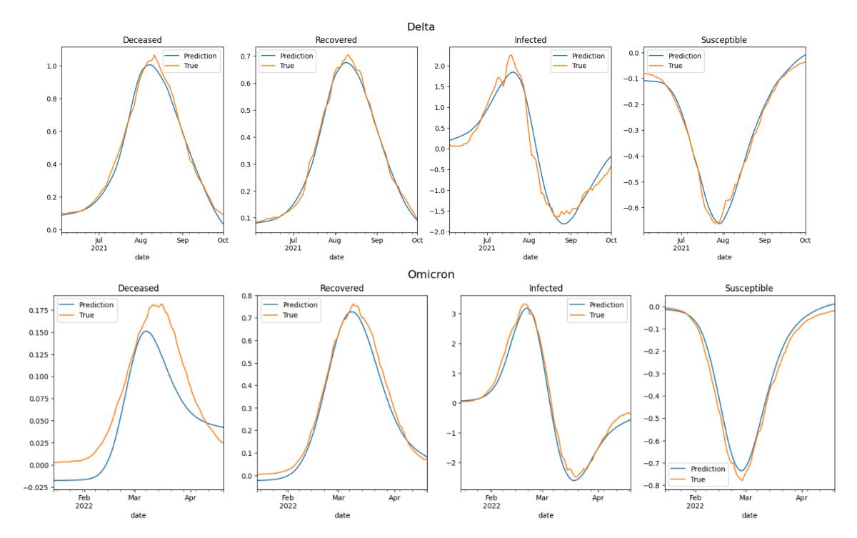
Figure 5: The curves of predicted gradient values of each compartment.
In Figure 6, the comparisons between the predicted values and the true values of all compartments are seen clearly. The prediction fit nicely in the profile of the true values. Despite some small differences it shows, the shape of the dynamics and the trends the SINDy model predicted agree to the true values, indicating
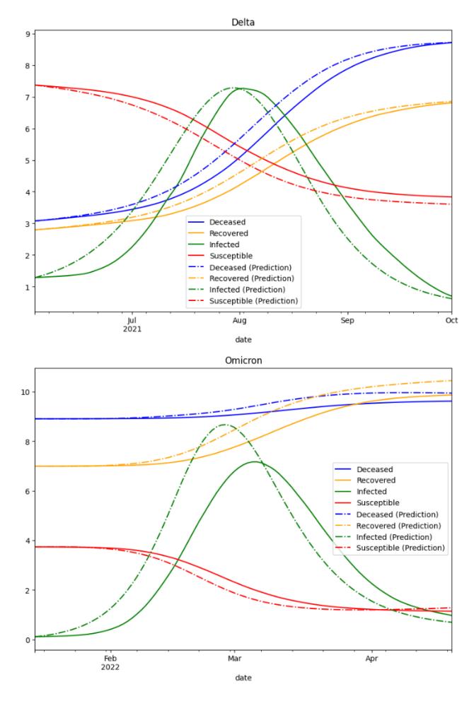
Figure 6: Curve of the integration results and the true values of each compartment during peak period of each variant.
that the SIRD system learned is valid. In the practical aspect, this model is then capable to predict the rise and fall of the pandemics by forecasting the trends of the infection. Significant discrepancies shown in the Infected curve are possibly caused by the lacks of complete data from other potential compartments used in the model. The exclusion of some compartments, such as second infection, can reduce model capacity, because there are some features that cannot be considered by the model. The other possible factor of the discrepancy is that there may be some higher-order of nonlinear interactions affecting the dynamics.
3.4. Weight analysis
One aspect of SINDy approach that cannot be ignored is its interpretability. The main target of SINDy is to predict the dynamical system itself, thus the parameter obtained should be sparse enough (but not too sparse) to have some meaningful interpretation. Previously, we have obtained that the best model is the one with L1 = 0.01. However, if we plot the parameters of the model in terms of polynomial coefficient of the system (shown in Figure 7(a)), almost every term is filled, giving less information regarding the system. For that matter, we retrain the model with different values of L1, but still without Ridge regularization to see the optimal values of L1 that gives enough sparsity. The complete results can be seen in Figure 7. We use heatmaps in the figure to easily show the dominant terms in the learned system where the parameter matrices are set to be sparse.
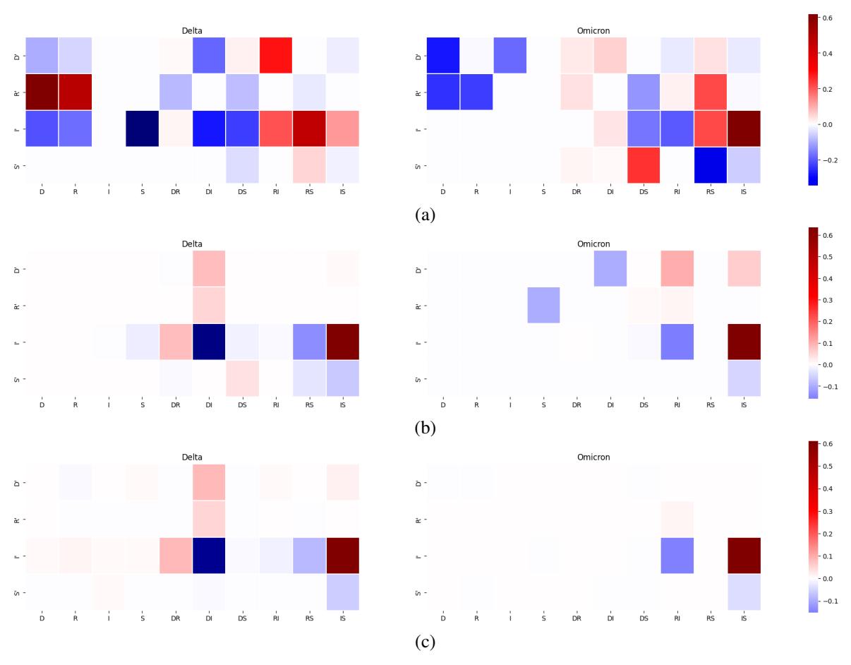
Figure 7: Heatmap of the weight parameters of the learned SIRD system with different regularization strengths, where (a) L1 = 0.01; (b) L1 = 0.02; (c) L1 = 0.05.
As mentioned, the one with L1 = 0.01 is not sparse enough. It may be representing some true complex systems, but in our case, we know that compartmental model should be simple. On the other hand, the one with L1 = 0.05 gives too sparse parameters that in the Omicron case, all the terms for the dynamics of R and D (almost) vanish, which should not be true in our case because we know that they have dynamics and is not constant all the time. So, we choose the middle value, L1 = 0.02 and obtained just the right sparsity. We see how, in the Omicron case for example, that death value is affected by terms DI, RI, and IS, or in simple words the "interaction" between the infected and other compartment, including the deceased itself. It is quite reasonable because the number of death may cause some kind of pessimism to the infected one and worsened the disease. The similar interpretation can also be done to other dynamics.
Further more, we can see that roughly some of the parameters that is activated in Omicron is also activated in Delta in different strength. Even thought there are also many terms that appears in one of the variant but does not appear in the other, they represent similar dynamics of how the number of infected people rises in parallel with the dynamics of other compartments. For instance, the increase of the deceased in Omicron period is relatively small compared to Delta period because Omicron system have negative terms of DI that balance the positive terms of RI and IS. On the other hand, infected people in Omicron period rise more quickly than Delta because the infected only depends on two terms where the Delta has some other terms that balance the increase.
4. CONCLUSION
This study introduced compartmental model, especially in form of SIRD model, for COVID-19 transmission dynamics, specifically during peak period of Delta and Omicron variants in Indonesia, constructed from empirical data. Model selection was based on comparing the mean squared error across various values of regularization. The resulting model demonstrated a high degree of accuracy in predicting real infection data, exhibiting only minor discrepancies. Despite its predictive prowess, the data-constructed model suffers from limited interpretability. Optimal value of regularization should consider the balance of explainability of the system obtained, represented by the map of its coefficients, and the error of the model. The challenges in directly interpreting the model stem from a multitude of intricate factors that indirectly impact real-world data. Hidden variables give rise to numerous nonlinear interactions between compartments, which the constructed model aims to capture. Enhancing the interpretability of data-constructed compartmental models is a key focus for future research endeavors. One potential avenue for improvement involves purposefully selecting a subset of favorable terms as features, as opposed to incorporating all polynomial terms of a given order. Additionally, the inclusion of supplementary intermediary compartments, such as those representing exposed individuals, incompletely vaccinated individuals, or hospitalized cases, could be considered contingent upon data availability.