

1. Introduction
Tuberculosis (TB) is an infectious disease caused by the bacterium Mycobacterium tuberculosis, which mostly affects the lungs [1], [3]. It gets transmitted when an infected person in the active TB disease stage in their lungs coughs, sneezes, or inhales the expelled droplets containing TB bacteria [1]. TB infections generally follow three stages: primary infection, when an individual is initially exposed to the TB bacterium; latent stage, if there is a delay in diagnosis or treatment such as preventive care; and active TB infection stage [2].
In recent times, TB has been a disease with high mortality (about 1.6 million TB deaths in 2021) as its global impact was felt in every region of the world, with the highest number of new cases being reported in the
*Corresponding author
Received November \(16^{th}\), 2023, Revised February \(25^{th}\), 2024, Accepted for publication June \(8^{th}\), 2024. Copyright ©2024 Published by Indonesian Biomathematical Society, e-ISSN: 2549-2896, DOI:10.5614/cbms.2024.7.1.4
WHO (World Health Organization) South-East Asian Region at 46%, followed by the WHO African Region at 23% and the WHO Western Pacific Region at 18% [3]. The 2021 WHO global statistics identified TB as the 13th leading cause of death and the second leading infectious killer after COVID-19 (above HIV/AIDS), with over 10.6 million people falling sick with TB. These infected populations include six million men, 3.4 million women, and 1.2 million children since TB exists in all countries and across age groups [3]. In South East Asia, Indonesia witnessed the highest number of TB cases as per the WHO.
According to the WHO report [3] in 2021, Indonesia, which had 9.2% of TB cases in the world, came second in the highest number of TB cases below India (28%) and above China (7.4%). Many interventions and supporting policies have been implemented by the Indonesian government to eliminate/minimize TB cases. In 2015, the elimination of TB was one of the priority programs by the President of Indonesia. With this policy, TB detection was conducted intensively with a district-based public-private mix policy.
TB is a complex disease, which makes the prevention strategy very challenging. Early TB case detection is a good strategy to identify TB cases in earlier stages and to stop the transmission [5]. This is achieved through the patient-initiated and screening pathways [7]. Techniques for early detection of TB include chest X-ray examination, the Mantoux tuberculin skin test, and TB blood tests (interferon-gamma release assay, QuantiFERON-TB Gold, and T-Spot). Among these, a chest X-ray examination is the best diagnosis/screening technique recommended for detecting pulmonary abnormalities, such as with TB, since it looks for changes in the lungs that could show signs of active TB or scars from previous TB infections [8]. Other methodologies for the early detection of tuberculosis outbreaks (through a statistical approach) are county-based log-likelihood ratio, cumulative sums, and spatial scan statistics [9]. Early detection/identification of epidemics such as those caused by TB has remained a critical component in reducing the global burden and has proven to be crucial in the fight to control the extent of TB outbreaks in many regions of the world where these techniques have been implemented to date [9]. Incidentally, directly observed treatment short-course (DOTS) is recommended by WHO as the most effective strategy for TB case detection and control nowadays. However, since the implementation of DOTS in 1955 in Indonesia, the number of new TB cases reported in hospitals has continued to be low [6].
Upon diagnosing TB in humans, the active case of TB disease can be treated with a combination of antibacterial administered for a duration between six to twelve months. The most common treatments for TB include the use of isoniazid (INH) in combination with three other drugs, namely rifampin, pyrazinamide, and ethambutol [4]. One of the risks to controlling TB is treatment failure, defined as a patient having a positive sputum smear or sputum culture at least five months after starting anti-TB treatment. This is due to both its link to multidrug-resistant TB (MDR TB) and still the fact that infected patients continue to disseminate the disease [10], [11].
Several modeling approaches have been used to gain insight into the early detection and understanding of the primary transmission dynamics of TB in the human population, and they provide valuable recommendations on various ways to limit/stop its spread and prevent it from developing to an advanced stage(s); see the following reference mathematical modeling approach [12], [13], [29], stochastic approach [16], statistical method [9], artificial intelligence [17], [19], and so on. In particular, Okuonghaem et al. [14] presented a qualitative and quantitative study of the TB mathematical model to assess four key factors that impact TB transmission, namely an effective awareness program, active cough identification, the associated cost factor of identified cases, and effective treatment applied for a survey TB data in Benin City, Nigeria. The results from their modeling indicate that improvement in case detection, constant implementation of awareness programs, and the use of active cough identification as markers for quick detection are vital in reducing the severity of TB in the presence of treatment. Authors in [12] studied a susceptible-exposed-infected-recovery (SIER) nonlinear mathematical model of TB with a special focus on analyzing the effect of case detection and treatment while assuming that susceptible individuals can move to become exposed or infected classes simultaneously based on their immunity level. The authors conducted a mathematical and numerical analysis that suggested that an increase in the rate of case detection shifts the backward bifurcation diagram toward the right, therefore leading to an increase in the threshold value of the basic reproduction number, while treatment reduces the equilibrium level of the infective population. Liu et al. [27] studied a mathematical model of tuberculosis incorporating treatment interruptions and two latent periods, which was an extension/modification of the work presented in [15] as they claimed that the latency period of tuberculosis could not be neglected because of its importance in analyzing TB models. Results from their modeling framework suggested that the reproduction numbers and numerical simulations show that the treatment of active TB cases always helps control the
TB epidemic, while treatment interruptions may have a negative, positive, or no effect on combating the TB epidemic. Furthermore, Lotfi et al. [28] used five systems of an ordinary differential equation (ODE) to capture and study the tuberculosis epidemic model with two treatments (i.e., those who fail and effectively treatment classes) and exogenous re-infection. Mathematical analysis of their model shows that there exists a backward bifurcation when the stable disease-free equilibrium coexists with a stable endemic equilibrium for the related basic reproduction number is less than one. Numerous mathematical models that have studied TB with a particular focus on understanding the transmission dynamics and with a possible prediction on TB controls are as follows: vaccinations and treatment [20], health education and early therapy [21], screening and treatment [22], transmission with children and adults groups [23], [18], the two-strain tuberculosis model in Bangladesh [24], diagnosis [32], parameter estimation [33], optimal control with re-infection and post-exposure interventions [25], and many others.
Previous discussions in many works in the literature suggest that early TB detection and proper treatment play a vital role in the TB elimination program. However, only a few mathematical models discuss these two important interventions. The present study's aim is to understand the impact of early TB detection in minimizing the number of TB cases in the long term of interventions. Furthermore, the study aims to find the minimum quality level of TB treatment success probability such that treatment can be used as a front-line intervention to combat TB. The rest of the article is structured as follows. The mathematical model constructed with a detailed assumption is given in Section 2. Parameter estimation using accumulated TB cases in Indonesia from 2017 to 2021 is discussed in Section 3. The mathematical model analysis to guarantee the well-defined properties of the proposed model is provided in Section 4. The same section offers a comprehensive analysis of the existence criteria of equilibrium points along with the respected control reproduction number. We show the non-existence of backward bifurcation of our model in section 5. Section 6 discusses some numerical experiments conducted, such as PRCC analysis, sensitivity analysis on the control reproduction number and endemic size, as well as autonomous simulations. Finally, Section 7 presents the conclusion.
2. MODEL FORMULATION
A mathematical model for TB transmission was formulated by dividing the population into six compartments; namely, susceptible individuals (S), latently undetected individuals \((E_1)\), latently detected individuals \((E_2)\), active TB individuals (I), imperfect recovered individuals and should take the second dose of treatment \((R_1)\), and perfect recovered individuals \((R_2)\). With this division, the total population (N) is governed by
\[N(t) = S(t) + E_1(t) + E_2(t) + I(t) + R_1(t) + R_2(t).\]
The transmission diagram used to construct the model is given in Figure 1. The susceptible compartment includes individuals at risk of TB infection, while perfectly recovered individuals are those who recently recovered from TB and have a temporal immunity \((\kappa^{-1})\) to TB infection. The authors assume that the susceptible compartment can get infected by TB due to contact with active TB individuals (I) and imperfectly recovered individuals \((R_1)\). We assume that the individuals in \(R_1\) compartment still have a chance to spread the disease since they failed in the previous treatment [26]. Assuming the probability of success infection given by \(\beta\) and the probability of fast and slow progression given by p and p respectively, the force of infection is given by:
\[F(I,R_1) = \text{slow progression case} + \text{fast progression case},\] \[= (1-p)\beta \frac{\eta I + R_1}{N} + p\beta \frac{\eta I + R_1}{N},\] \[= \beta \frac{\eta I + R_1}{N} S,\] (1)
where \(\eta \in (0,1]\) is the correction parameter of infection for I individuals. The first intervention implemented in the model is the case detection \(u_1\), which is given to detect the existence of latent individuals. It is assumed that the undetected latent individuals \(E_1\) do not get treatment, while the detected latent individuals \(E_2\) get the first dose of treatment. If the treatment fails, then the infection status of an individual of \(E_2\) will increase to the active infected patient in the I compartment. The duration of the first dose of treatment is \(\delta_1^{-1}\). The
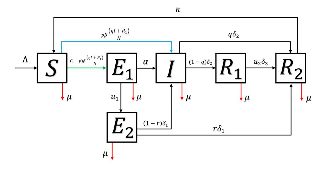
Figure 1: Transmission diagram of TB transmission model in (2).
probability of treatment success for \(E_2\) is assumed to be \(r \in [0,1]\). The progression rate of \(E_1\) to become active TB is \(\alpha\). Similar to \(E_2\), it is also possible that the active TB individuals \(I_2\) who received the advanced first dose of treatment failed the treatment. The probability of treatment success is assumed to be \(q \in [0,1]\), with the duration of the second dose treatment being \(\delta_2^{-1}\). Lastly, it is assumed that the third dose treatment duration for an imperfectly recovered individual is \(\delta_3^{-1}\), with successful probability \(u_2\). Based on the above model description and the transmission diagram in Figure 1, the governing model can be developed as a system of nonlinear differential equations given as follows:
\[\frac{dS}{dt} = \Lambda + \kappa R_2 - (1 - p)\beta S \frac{(\eta I + R_1)}{N} - p\beta S \frac{(\eta I + R_1)}{N} - \mu S,\] (2a) \[\frac{dE_1}{dt} = (1 - p)\beta S \frac{(\eta I + R_1)}{N} - u_1 E_1 - \alpha E_1 - \mu E_1,\] (2b)
\[\frac{dE_1}{dt} = (1 - p)\beta S \frac{(\eta I + R_1)}{N} - u_1 E_1 - \alpha E_1 - \mu E_1, \tag{2b}\]
\[\frac{dE_2}{dt} = u_1 E_1 - (1 - r)\delta_1 E_2 - r\delta_1 E_2 - \mu E_2,\] (2c)
\[\frac{dI}{dt} = u_1 E_1 - (1 - r)\delta_1 E_2 - r\delta_1 E_2 - \mu E_2,\] \[\frac{dI}{dt} = p\beta S \frac{(\eta I + R_1)}{N} + (1 - r)\delta_1 E_2 + \alpha E_1 - q\delta_2 I - (1 - q)\delta_2 I - \mu I,\] (2d)
\[\frac{dR_1}{dt} = (1 - q)\delta_2 I - u_2 \delta_3 R_1 - \mu R_1, \frac{dR_2}{dt} = u_2 \delta_3 R_1 + r \delta_1 E_2 + q \delta_2 I - \kappa R_2 - \mu R_2,\] (2e)
\[\frac{dR_2}{dt} = u_2 \delta_3 R_1 + r \delta_1 E_2 + q \delta_2 I - \kappa R_2 - \mu R_2, \tag{2f}\] with initial conditions:
\[S(0) > 0\], \(E_1(0) \ge 0\), \(E_2(0) \ge 0\), \(I(0) \ge 0\), \(R_1(0) \ge 0\), \(R_2(0) \ge 0\).
The description and values of each parameter in model (2) are given in Table 1.
3. PARAMETER ESTIMATION
To fit and estimate the model parameters in system (2), the "lsqnonlin" built-in function in MATLAB was used. The "lsqnonlin" function in MATLAB is part of the Optimization Toolbox and is primarily
| Parameters | Description | Value | Source |
|---|---|---|---|
| Λ | Recruitment rate to the population | 270 200 000 human 71.5×4 quarter year | [30], [31] |
| \(\beta\) | Probability of successful infection rate | 1.3 \(\frac{1}{\text{quarter year}}\) | Estimated |
| \(u_1\) | Case detection rate | 1 1 quarter year | Estimated |
| \(u_2\) | Probability of second dose treatment success | 0.7 | Estimated |
| \(\eta\) | Correction parameter for transmission rate I | 0.12 | Estimated |
| p | Probability of fast progression | 0.063 | [32] |
| \(\alpha\) | Progression rate of undetected latent individuals | \(0.3 \frac{1}{\text{quarter year}}\) | [34] |
| \(\delta_1\) | Recovery rate of detected latent individuals | \(0.8745 \frac{1}{\text{quarter year}}\) | [35] |
| \(\delta_2\) | Recovery rate of active infected individuals | \(0.5415 \frac{1}{\text{quarter year}}\) | [35] |
| \(\delta_3\) | Recovery rate of imperfectly recovered individuals | \(0.158 \frac{1}{\text{quarter year}}\) | [36] |
| \(\mu\) | Natural death rate | \(\frac{1}{71.5 \times 4}\) \(\frac{1}{\text{quarter year}}\) | [31] |
| \(\kappa\) | Waning rate of immunity | \(0.875 \frac{1}{\text{quarter year}}\) | [37] |
| r | Probability of successful first dose treatment | 0.9 | Estimated |
| q | Probability of successful advanced first dose treatment | 0.8 | Estimated |
Table 1: Parameter description, values, and sources.
used for solving nonlinear least squares problems. Nonlinear least squares problems involve minimizing the sum of the squares of nonlinear functions. This optimization problem arises in various fields, including curve fitting, parameter estimation, and data fitting. For more explanation and examples on the use of this method, readers can see [38].
The data sources for this study consist of accumulated quarterly incidence data of Tuberculosis (TB) in Indonesia spanning from 2017 to 2021. These data were obtained by personal request to the Ministry of Health, Indonesia. It's worth noting that Indonesia has a considerable population estimated at around 270 million individuals. The decision to use quarterly time steps, as opposed to weekly, daily, or monthly intervals, was made since this is the best incidence data that was available from the mentioned source.
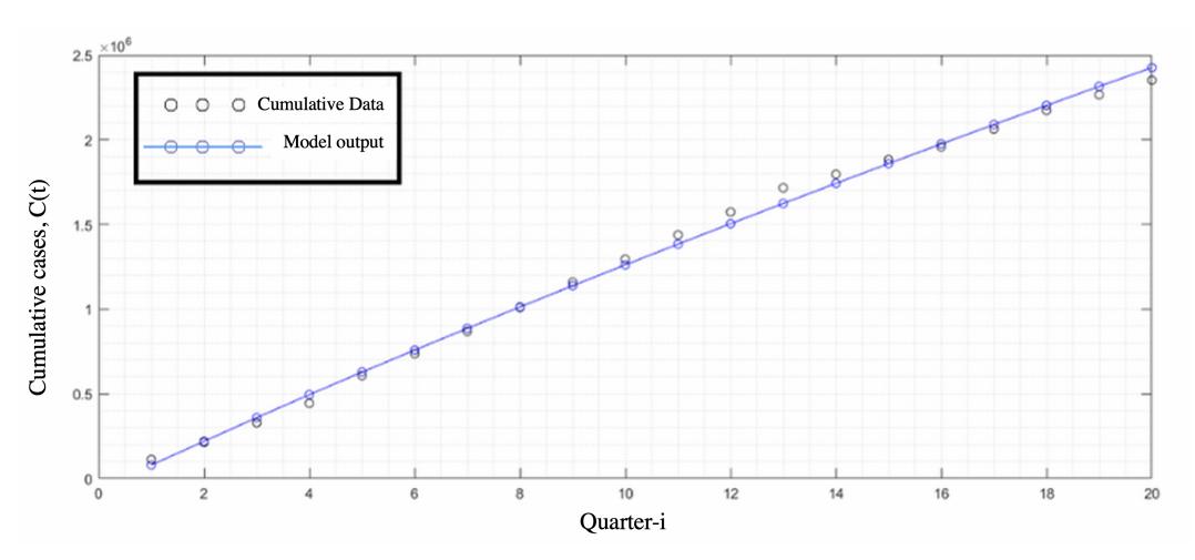
Figure 2: The fitted accumulated data, C(t).
Here, the authors wanted to estimate the infection rate \(\beta\), case detection rate \(u_1\), probability of successful second dose treatment \(u_2\), correction parameter of infection rate of actively infected individuals \(\eta\), probability of successful first dose treatment r, and the probability of successful advanced first dose treatment q, as well as the best initial condition for the proposed model. Our aim was to find the best-fit parameter such that the squared error between simulation results and the accumulated incidence data in the field, which is given by
\[C = \int_0^T \left[ u_1 E_1 + p\beta S \frac{(\eta I + R_1)}{N} + \alpha E_1 \right] dt,\]
could be as minimum as possible, where C is the accumulated infected individuals. Assuming the best-fit parameters are \(\beta^*, u_1^*, u_2^*, \eta^*, r^*\), and \(q^*\) and the best-fit initial condition \(X^0\), the aim was to minimize the following function
\[RMSE = \sqrt{\frac{1}{20}\sum_{i=1}^{20}(C_{\mathrm{prediction}_i} - C_{\mathrm{data}_i})^2},\] where 20 is the number of accumulated data points that are available. From the simulation, it was found that the proposed model fit well to the data as shown in Figure 2. The best fit parameters of model (2) are given in Table 1, while the best-fit initial condition is given by
\[S(0) = 257\,900\,037, \ E_1(0) = 9,964, \ E_2(0) = 12\,501, \ I(0) = 12\,501, \ R_1(0) = 112\,494, \ R_2(0) = 195\,253.\]
4. QUALITATIVE ANALYSIS
4.1. Basic properties
Since we are dealing with human populations, it is important that all solutions of the proposed model must be positive and bounded in a feasible region. To satisfy this condition, the following propositions were made:
Proposition 1. The solution of model (2) is non-negative for t > 0 if the initial condition satisfies
\[S(0) > 0\], \(E_1(0) \ge 0\), \(E_2(0) \ge 0\), \(I(0) \ge 0\), \(R_1(0) \ge 0\), \(R_2(0) \ge 0\).
Proof: From the first equation of system (2), we have the following inequality:
\[\frac{dS}{dt} \ge -\left((1-p)\beta \frac{(\eta I + R_1)}{N} + p\beta \frac{(\eta I + R_1)}{N} + \mu\right) S. \tag{3}\]
Using the integrating factor
\[\exp \int_0^t -\left((1-p)\beta \frac{(\eta I(\tau) + R_1(\tau))}{N(\tau)} + p\beta \frac{(\eta I(\tau) + R_1)}{N(\tau)} + \mu\right) d\tau\] in (3), we have
\[S(t) > S(0) \exp \int_0^t -\left( (1-p)\beta \frac{(\eta I(\tau) + R_1(\tau))}{N(\tau)} + p\beta \frac{(\eta I(\tau) + R_1)}{N(\tau)} \right) d\tau + \mu t > 0,\]
for all t > 0. The proof for remaining variables \(E_1, E_2, I, R_1\), and \(R_2\) can be shown in a similar way. Hence, it can be concluded that the solution of all variables in model (2) is always non-negative for all time t > 0.
Proposition 2. The feasible region \(\Omega\) defined by
\[\Omega = \left\{ (S, E_1, E_2, I, R_1, R_2) \in \mathbb{R}^6_+ : N(t) \le \frac{\Lambda}{\mu} \right\}\] is positively invariant under system (2).
Proof: Summing up the human population compartment gives
\[\frac{dN}{dt} = \Lambda - \mu N.\]
Consequently,
\[N = \frac{\Lambda}{\mu} (1 - \exp(-\mu t)) + N(0) \exp(-\mu t).\]
Taking the lim sup as \(t\to\infty\) gives \(N=\frac{\Lambda}{\mu}\). Furthermore, if \(N(0)\leq\frac{\Lambda}{\mu}\), then for all t>0, we have \(N(t)\leq\frac{\Lambda}{\mu}\). However, if \(N(0)>\frac{\Lambda}{\mu}\), then the solution of N(t) approaches \(\Omega\). Therefore, it follows that the region \(\Omega\) is positively invariant and attractive.
The implication of the above two propositions is that model (2) is mathematically well-posed in the epidemiologically feasible region \(\Omega\).
4.2. Equilibrium points and the control reproduction number
The first analysis in this section seeks to determine the equilibrium points of system (2) by solving
\[\frac{dS}{dt} = \frac{dE_1}{dt} = \frac{dE_2}{dt} = 0, \frac{dI}{dt} = 0, \frac{dR_1}{dt} = 0, \frac{dR_2}{dt} = 0,\]
respective to each variables \(S, E_1, E_2, I, R_1\), and \(R_2\). By solving this problem, the TB model in system (2) has two types of equilibrium, namely the TB-free equilibrium (denoted by \(\mathbf{x}^*\)) and the TB-endemic equilibrium (denoted by \(\mathbf{x}^*\)). The TB-free equilibrium point of system (2) is given by
\[\mathbf{x}^\dagger = \left(S^\dagger, E_1^\dagger, E_2^\dagger, I^\dagger, R_1^\dagger, R_2^\dagger\right) = \left(\frac{\Lambda}{\mu}, 0, 0, 0, 0, 0\right).\]
The linear stability of \(\mathbf{x}^*\) is established using the concept of the basic reproduction number. Basic reproduction number, \(\mathcal{R}_0\), is the endemic indicator for a disease transmission, which presents the expected number of secondary cases due to one primary case in a completely susceptible population during the infection period [39]. Many epidemiological models [40], [41], [42], [43], [44] have used the concept of \(\mathcal{R}_0\) to determine whether their model tends to the free disease state or endemic state. Most of them found that the disease has a chance to get eradicated if \(\mathcal{R}_0 < 1\), and persist if \(\mathcal{R}_0 > 1\). We calculate the control reproduction number using the concept of the next-generation matrix approach introduced by authors in [45]. At first, we linearize our sub-system infected compartment of model (2) in \(\mathbf{x}^*\), which only involve \(\frac{d\mathcal{E}_1}{dt}, \frac{d\mathcal{E}_2}{dt}, \frac{dI}{dt}\), and \(\frac{dR_1}{dt}\). Let's define the matrix \(\mathcal{J}\). By separating the transmission term (\(\mathcal{F}\)) and transition term (\(\mathcal{V}\)) of \(\mathcal{J}\), where \(\mathcal{J} = \mathcal{F} + \mathcal{V}\), we have
\[\mathcal{F} = \begin{bmatrix} 0 & 0 & (1-p)\beta\eta & (1-p)\beta \\ 0 & 0 & 0 & 0 \\ 0 & 0 & p\beta\eta & p\beta \\ 0 & 0 & 0 & 0 \end{bmatrix},\] and
\[\mathcal{V} = \begin{bmatrix} -u_1 - \alpha - \mu & 0 & 0 & 0 \\ u_1 & -(1-r)\delta_1 - r\delta_1 - \mu & 0 & 0 \\ \alpha & (1-r)\delta_1 & -q\delta_2 - (1-q)\delta_2 - \mu & 0 \\ 0 & 0 & (1-q)\delta_2 & -u_2\delta_3 - \mu \end{bmatrix}.\]
Since the second and fourth row of \(\mathcal{F}\) are zero, we define
\[\mathbf{E} = \begin{bmatrix} 1 & 0 \\ 0 & 0 \\ 0 & 1 \\ 0 & 0 \end{bmatrix},\]
such that the next-generation matrix of the proposed TB model in (2) is given by
\[\mathbf{K} = -E^T \mathcal{F} \mathcal{V}^{-1} E,\] \[= \begin{bmatrix} k_{11} & k_{12} \\ k_{21} & k_{22} \end{bmatrix},\] where
\[\begin{split} k_{11} &= \frac{\left(1-p\right)\eta\beta\left(\delta_{1}u_{1}(1-r)+\alpha\mu+\alpha\delta_{1}\right)}{\left(\mu+\delta_{2}\right)\left(\mu+\delta_{1}\right)\left(u_{1}+\alpha+\mu\right)} - \frac{\left(1-p\right)\beta L}{\left(u_{1}+\alpha+\mu\right)\left(\mu+\delta_{1}\right)\left(\mu+\delta_{2}\right)\left(u_{2}\delta_{3}+\mu\right)},\\ k_{12} &= \frac{\left(1-p\right)\eta\beta}{\delta_{2}+\mu} + \frac{\left(1-p\right)\beta\left(1-q\right)\delta_{2}}{\left(\mu+\delta_{2}\right)\left(u_{2}\delta_{3}+\mu\right)},\\ k_{21} &= \frac{p\beta\eta\left(\delta_{1}u_{1}(1-r)+\alpha\mu+\alpha\delta_{1}\right)}{\left(\mu+\delta_{2}\right)\left(\mu+\delta_{1}\right)\left(u_{1}+\alpha+\mu\right)} - \frac{p\beta L}{\left(u_{1}+\alpha+\mu\right)\left(\mu+\delta_{1}\right)\left(\mu+\delta_{2}\right)\left(u_{2}\delta_{3}+\mu\right)},\\ k_{22} &= \frac{p\beta\eta}{\delta_{2}+\mu} + \frac{p\beta\left(1-q\right)\delta_{2}}{\left(\mu+\delta_{2}\right)\left(u_{2}\delta_{3}+\mu\right)}, \end{split}\] with
\[L = (-qr\delta_1u_1 + \alpha\mu q + \alpha q\delta_1 + q\delta_1u_1 + r\delta_1u_1 - \alpha\mu - \alpha\delta_1 - \delta_1u_1)\delta_2.\]
Hence, the control reproduction number of model (2) is taken from the spectral radius of K and given by
\[\mathcal{R}_{0} = \frac{\beta \left( \eta \, \delta_{3} u_{2} + \eta \, \mu + \delta_{2} (1 - q) \right) \left( p r \delta_{1} u_{1} + \mu^{2} p + \mu \, p \delta_{1} + \mu \, p u_{1} + \alpha \, \mu + \alpha \, \delta_{1} + \delta_{1} u_{1} (1 - r) \right)}{\left( u_{2} \delta_{3} + \mu \right) \left( \delta_{2} + \mu \right) \left( \mu + \delta_{1} \right) \left( u_{1} + \mu + \alpha \right)}.\]
In the absence of control parameters \(u_1\) and \(u_2\), the control reproduction number \((\mathcal{R}_0)\) reduced into the basic reproduction number \((\mathcal{R}_0^*)\) given by
\[\mathcal{R}_0^* = \frac{\beta(\eta\mu + \delta_2(1-q))(\mu p + \alpha)}{(\delta_2 + \mu)(\mu + \alpha)}.\]
4.3. Stability of the TB-free equilibrium point
1) Local stability of the TB-free equilibrium: The local stability of the TB-free equilibrium points is given by the following theorem.
Theorem 1. The TB-free equilibrium point of system (2) is locally asymptotically stable if \(\mathcal{R}_0 < 1\) and unstable if \(\mathcal{R}_0 > 1\).
Proof: To proof this theorem, the result in [46] is used by showing that the proposed model satisfies five axioms in [46]. First, let us define model (2) as follows:
\[\frac{dI}{dt} = p\beta S \frac{(\eta I + R_1)}{N} + (1 - r)\delta_1 E_2 + \alpha E_1 - q\delta_2 I - (1 - q)\delta_2 I - \mu I = f_1, \tag{4a}\]
\[\frac{dR_1}{dt} = (1 - q)\delta_2 I - u_2 \delta_3 R_1 - \mu R_1 = f_2, \tag{4b}\]
\[\frac{dE_1}{dt} = (1 - p)\beta S \frac{(\eta I + R_1)}{N} - u_1 E_1 - \alpha E_1 - \mu E_1 = f_3, \tag{4c}\]
\[\frac{dE_2}{dt} = u_1 E_1 - (1 - r)\delta_1 E_2 - r\delta_1 E_2 - \mu E_2 = f_4,\tag{4d}\]
\[\frac{dR_2}{dt} = u_2 \delta_3 R_1 + r \delta_1 + q \delta_2 I - \kappa R_2 - \mu R_2 = f_5, \tag{4e}\]
\[\frac{dS}{dt} = \Lambda + \kappa R_2 - (1-p)\beta S \frac{(\eta I + R_1)}{N} - p\beta S \frac{(\eta I + R_1)}{N} - \mu S = f_6. \tag{4f}\]
Next, we define the TB-free equilibrium as follows:
\[\mathbf{X_s} = \left\{ x_1 = I = 0, x_2 = R_1 = 0, x_3 = E_1 = 0, x_4 = E_2 = 0, x_5 = R_2 = 0, x_6 = S = \frac{\Lambda}{\mu} \right\}.\]
The new infection (transmission) part of system (4) is given by
\[\bm{\mathcal{F}}(\bm{x}) = \left[ \begin{array}{c} p\beta S \frac{(\eta I + R_1)}{N} \\ 0 \\ (1 - p)\beta S \frac{(\eta I + R_1)}{N} \\ 0 \\ 0 \\ 0 \end{array} \right],\] and the transition part is given by
\[\mathcal{V}(\mathbf{x}) = \begin{bmatrix} (\delta_2 + \mu)I - (1 - r)\delta_1 E_2 - \alpha E_1 \\ (u_2 \delta_3 + \mu)R_1 - (1 - q)\delta_2 I \\ (u_1 + \alpha + \mu)E_1 \\ \delta_1 E_2 + \mu E_2 - u_1 E_1 \\ (\kappa + \mu)R_2 - u_2 \delta_3 R_1 - r\delta_1 - q\delta_2 I \\ \beta S \frac{(\eta I + R_1)}{N} + \mu S - \kappa R_2 - \Lambda \end{bmatrix},\] \[= \begin{bmatrix} (\delta_2 + \mu)I \\ (u_2 \delta_3 + \mu)R_1 \\ (u_2 \delta_3 + \mu)R_1 \\ (u_1 + \alpha + \mu)E_1 \\ \delta_1 E_2 + \mu E_2 \\ (\kappa + \mu)R_2 \\ \beta S \frac{(\eta I + R_1)}{N} + \mu S \end{bmatrix} - \begin{bmatrix} (1 - r)\delta_1 E_2 + \alpha E_1 \\ (1 - q)\delta_2 I \\ 0 \\ u_1 E_1 \\ u_2 \delta_3 R_1 + r\delta_1 + q\delta_2 I \\ \kappa R_2 + \Lambda \end{bmatrix},\] \[= \mathcal{V}^-(\mathbf{x}) - \mathcal{V}^+(\mathbf{x}),\] where \(V_i^-\) and \(V_i^+\) present the out- and in- flow of each compartment, respectively. Now, we proof the five axioms in [46] to guarantee the LAS properties of the TB-free equilibrium.
- 1) If all compartments are non-negative, then \(\mathcal{F}_i, \mathcal{V}_i^-\), and \(\mathcal{V}_i^+\) are always non-negative. Proof: By substituting \(S>0, E_1>0, E_2>0, I>0, R_1>0\) and \(R_2>0\), into \(\mathcal{F}_i, \mathcal{V}_i^-\), and \(\mathcal{V}_i^+\), it can be seen trivially that \(\mathcal{F}_i, \mathcal{V}_i^-\), and \(\mathcal{V}_i^+\) are always non-negative.
- 2) If all compartments are zero, then \(\mathcal{V}_i^- = 0\) for i = 1, 2, ... 6. Furthermore, if all variables are at \(X_s\), then \(\mathcal{V}_i^- = 0\) for i = 1, 2, 3, 4. Proof: It is easy to verify that \(\mathcal{V}_i^- = 0\) for i = 1, 2, ... 6 when we set \(S = E_1 = E_2 = I = R_1 = R_2 = 0\). Furthermore, when we substitute \(X_s\) into \(\mathcal{V}_i\) for i = 1, 2, 3, 4, then we have \(V_i = 0\).
- 3) F<sub>i</sub> = 0 for i=5,6. Proof: This is trivial directly from the expression of F<sub>5</sub> and F<sub>6</sub>. 4) If x<sub>i</sub> ∈ X<sub>s</sub>, then F<sub>i</sub> = 0 and V<sub>i</sub><sup>+</sup> = 0 for i = 1, 2, 3, 4. Proof: By substituting X<sub>s</sub> into F<sub>i</sub>, i = 1, 2, 3, 4, we have that F<sub>i</sub> = 0 and V<sub>i</sub><sup>+</sup> = 0, i = 1, 2, 3, 4.
- If \(\mathcal{F}(x) = 0\), then all the eigenvalues of \(Df(\mathbf{X_s})\), where \(Df(\mathbf{X_s})\) is the Jacobian matrix of system (4) evaluated at \(X_s\), have a negative real part. Proof: By substituting \(X_s\) and \(\mathcal{F}(x) = 0\) into system (4),
\[f_{1} = \frac{dI}{dt} = (1 - r)\delta_{1}E_{2} + \alpha E_{1} - (\delta_{2} + \mu)I,\] \[f_{2} = \frac{dR_{1}}{dt} = (1 - q)\delta_{2}I - u_{2}\delta_{3}R_{1} - \mu R_{1},\] \[f_{3} = \frac{dE_{1}}{dt} = -u_{1}E_{1} - \alpha E_{1} - \mu E_{1},\] \[f_{4} = \frac{dE_{2}}{dt} = u_{1}E_{1} - \delta_{1}E_{2} - \mu E_{2},\] \[f_{5} = \frac{dR_{2}}{dt} = u_{2}\delta_{3}R_{1} + r\delta_{1} + q\delta_{2}I - \kappa R_{2} - \mu R_{2},\] \[f_{6} = \frac{dS}{dt} = \Lambda + \kappa R_{2} - \beta S \frac{(\eta I + R_{1})}{N} - \mu S.\]
Hence, we have
\[Df(\mathbf{X_s}) = \begin{bmatrix} G_1 & 0 & \alpha & (1-r)\,\delta_1 & 0 & 0\\ (1-q)\,\delta_2 & G_2 & 0 & 0 & 0 & 0\\ 0 & 0 & G_3 & 0 & 0 & 0\\ 0 & 0 & u_1 & G_4 & 0 & 0\\ q\delta_2 & u_2\delta_3 & 0 & 0 & G_5 & 0\\ -\frac{\beta\,S\eta}{N} & -\frac{\beta\,S}{N} & 0 & 0 & \kappa & -\mu \end{bmatrix},\] where \(G_1 = -\delta_2 - \mu\), \(G_2 = -u_2 \delta_3 - \mu\), \(G_3 = -\alpha - \mu - u_1\), \(G_4 = -\mu - \delta_1\), \(G_5 = -\kappa - \mu\), and \(G_6 = -\mu\). By standard calculation, we obtain the eigenvalues of \(Df(\mathbf{X_s})\), namely \(-\mu\), \(-(\mu + u_2\delta_3)\), \(-(\alpha + \mu + u_3\delta_3)\)\(u_1\), \(-(\mu + \delta_1)\), \(-(\kappa + \mu)\), and \(-\mu\). Since all parameters are non-negative, all eigenvalues are negative. Since all five axioms in [46] were satisfied by the proposed model, we conclude that the TB-free equilibrium is locally stable if \(\mathcal{R}_0 < 1\) and unstable if \(\mathcal{R}_0 > 1\). Hence, the proof is completed.
2) Global stability of the TB-free equilibrium:
Theorem 2. The TB-free equilibrium is globally asymptotically stable if \(\mathcal{R}_0 < 1\).
Proof: We show that model (2) is globally asymptotically stable (GAS) using the method described in [47]. First, we re-write system (2) as follows, let
\[\begin{cases} \frac{dX}{dt} &= F(X,\mathcal{I}), \\ \frac{d\mathcal{I}}{dt} &= \mathcal{G}(X,\mathcal{I}) \ \mathcal{G}(X,0) = 0, \end{cases}\]
for \(X=\left(S,R_{2}\right)\in\mathbb{R}^{2}\) and \(\mathcal{I}=\left(E_{1},E_{2},I,R_{1}\right)\in\mathbb{R}^{5},\) where X and \(\mathcal{I}\) represent the classes of the uninfectious and infectious individuals respectively. Next, we redefine the DFE as
\[\mathfrak{M}^* = (X_0, 0) = \left(S^*, E_1^*, E_2^*, I^*, R_1^*, R_2^*\right) = \left(\frac{\Lambda}{\mu}, 0, 0, 0, 0, 0, 0\right).\]
According to [47], our TB model given in (2) will be GAS at \(\mathfrak{M}^*\) if the following conditions:
\[\mathfrak{C}_1\]. \(\mathfrak{M}^*\) is locally stable if \(\mathcal{R}_0 < 1\), \(\mathfrak{C}_2\). At \(\frac{dX}{dt} = F(X_0, 0)\) the DFE is GAS,
\(\mathfrak{C}_3\). \(\mathcal{G}(X,\mathcal{I}) = \mathcal{A}\mathcal{I} - \hat{\mathcal{G}}(X,\mathcal{I}), \ \hat{\mathcal{G}}(X,\mathcal{I}) \geq 0\) for \((X,\mathcal{I}) \in \Omega\), where \(\mathcal{A} = \mathcal{D}_{\mathcal{I}}\mathcal{G}(X,\mathcal{I})\) is a Metzler matrix and \(\Omega\) is the proposed model's feasible region, are satisfied. Now, we establish that our model satisfies each of the above-enumerated conditions \(\mathfrak{C}_1\) to \(\mathfrak{C}_3\)to guarantee the GAS of the DFE. Clearly, since the model, basic reproduction number, \(\mathcal{R}_0\), is calculated
using the approach in Van den Driessche, and Watmough [45], it implies that \(\mathfrak{M}^0\) is locally asymptotically stable whenever \(\mathcal{R}_0 < 1\). Suppose \(\Psi_0 = (\mu + u_1 + \alpha), \ \Psi_1 = \left(\mu + (1-r)\delta_1 + r\delta_1\right)\),
\(\Psi_2=(\mu+q\delta_2+(1-q)\delta_2),\ \Psi_3=(\mu+u_2\delta_3),\ \Psi_4=(\mu+k),\ \text{and}\ \lambda=\frac{\beta(\eta I+R_1)}{N}\cdot \text{Re-defining system}\) (2) as to follow the form given in equation (6), we obtain
\[\frac{dX}{dt} = F(X, \mathcal{I}) = \begin{pmatrix} \Lambda + \kappa R_2 - \left( (1 - p)\lambda + p\lambda + \mu \right) S \\ u_2 \delta_3 R_1 + r \delta_1 E_2 + q \delta_2 I - \Psi_4 R_2 \end{pmatrix},\]
\[\frac{d\mathcal{I}}{dt} = G(X, \mathcal{I}) = \begin{pmatrix} (1-p)\lambda S - \Psi_0 E_1 \\ u_1 E_1 - \Psi_1 E_2 \\ p\lambda S + (1-r)\delta_1 E_2 + \alpha E_1 - \Psi_2 I \\ (1-q)\delta_2 I - \Psi_3 R_1 \end{pmatrix},\] and
\[F(X,0) = \begin{pmatrix} \lambda - \mu S \\ 0 \end{pmatrix},\] whose solutions yield a unique equilibrium point \(\left(\frac{\Lambda}{\mu},0,0,0,0,0\right)\), thus being GAS, and therefore \(\mathfrak{C}_2\) is satisfied. Linearizing the above second matrix gives a Metzler matrix as follows:
\[\mathcal{A} = \mathcal{D}_{\mathcal{I}}(\mathfrak{M}^*, 0) = \begin{pmatrix} -\Psi_0 & 0 & \frac{\beta(1-p)\eta S^0}{N^0} & \frac{\beta(1-p)S^0}{N^0} \\ u_1 & -\Psi_1 & 0 & 0 \\ \alpha & (1-r)\delta_1 & \frac{\beta p\eta S^0}{N^0} - \Psi_2 & \frac{\beta pS^0}{N^0} \\ 0 & 0 & (1-q)\delta_2 & -\Psi_3 \end{pmatrix}.\]
Solving for \(\hat{\mathcal{G}}(X,\mathcal{I})\) and performing some algebraic manipulation yield
\[\hat{\mathcal{G}}(X,\mathcal{I}) = \mathcal{A}\mathcal{I} - \hat{\mathcal{G}}(X,\mathcal{I}) := \begin{pmatrix} \beta(1-p)(\eta I + R_1) \left[ \frac{S^0}{N^0} - \frac{S}{N} \right] \\ 0 \\ \beta p(\eta I + R_1) \left[ \frac{S^0}{N^0} - \frac{S}{N} \right] \\ 0 \end{pmatrix}.\]
Consequently,
\[\hat{\mathcal{G}}(X,\mathcal{I}) \ge \begin{pmatrix} \beta(1-p)(\eta I + R_1)S^0 \left[ \frac{1}{N^0} - \frac{1}{N} \right] \\ 0 \\ \beta p(\eta I + R_1)S^0 \left[ \frac{1}{N^0} - \frac{1}{N} \right] \\ 0 \end{pmatrix}\]
since \(\left(\frac{1}{N^0} - \frac{1}{N}\right) = \frac{N - N^0}{NN^0}\) and \(N(t) - N^0 = \left(\frac{\Lambda}{\mu} - N(0)\right) \exp(-\mu t)\) is positive. We have that \(\hat{\mathcal{G}}(X,\mathcal{I}) \geq 0\), and \(\mathfrak{C}_3\) is satisfied as well. All the three conditions \(\mathfrak{C}_1\) to \(\mathfrak{C}_3\) are satisfied, and therefore, we can conclude that the DFE of the model system (2) is GAS whenever \(\mathcal{R}_0 < 1\), which completes the proof.
4.4. Endemic equilibrium point
The next equilibrium point of system (2) is the endemic equilibrium point, which is given by
\[EE = (S^*, E_1^*, E_2^*, I^*, R_1^*, R_2^*),\] (6)
where
\[\begin{split} S^* &= \frac{\Lambda \left(\mu \delta_3 u_2 + \delta_2 \delta_3 u_2 + \mu^2 + \mu \delta_2\right) \left(\alpha \mu + \alpha \delta_1 + \mu^2 + \mu \delta_1 + \mu u_1 + \delta_1 u_1\right)}{\mu \beta \left(\eta \mu + (1-q) \, \delta_2 + \eta \delta_3 u_2\right) \left(p r \delta_1 u_1 + \mu^2 p + \mu p \delta_1 + \mu p u_1 + (1-r) \, \delta_1 u_1 + \alpha \mu + \alpha \delta_1\right)}, \\ E_1^* &= \frac{I^* \left(\delta_2 + \mu\right) \left(1-p\right) \left(\delta_1 + \mu\right)}{\left(\left(r(1-p)+1\right) u_1 + \mu p + \alpha\right) \, \delta_1 + \mu \left(\mu p + p u_1 + \alpha\right)}, \\ E_2^* &= \frac{u_1 E_1^*}{\delta_1 + \mu}, \\ R_1^* &= \frac{I^* \, \delta_2 \left(1-q\right)}{\delta_3 u_2 + \mu}, \\ R_2^* &= \frac{q \delta_2 I^* + r \delta_1 E_2^* + u_2 \delta_3 R_1^*}{\kappa + \mu}, \end{split}\] and \(I^* = \frac{a_0}{a_1}\), where
\[a_0 = (\mathcal{R}_0 - 1) (\delta_3 u_2 + \mu) (\mu + \delta_2) (\mu + \delta_1) (u_1 + \alpha + \mu),\]
\[a_1 = (L_1 + L_2 + L_3 + L_4 + L_5 + L_6 + L_7),\] with
\[\begin{split} L_1 &= (1-q)\,\kappa\,pr\delta_1\delta_2u_1 + (1-q)\,\kappa\,\delta_1\delta_2u_1 + \kappa\,qr\delta_1\delta_2u_1 + \kappa\,r\delta_1\delta_2u_1 + \mu\,\delta_1\delta_2u_1, \\ L_2 &= (1-r)\,\kappa\,\delta_1\delta_3u_1u_2 + \kappa\,pr\delta_1\delta_3u_1u_2 + \mu\,\delta_1\delta_3u_1u_2 + (1-q)\,\alpha\,\kappa\,\mu\,\delta_2, \\ L_3 &= (1-pq)\,\kappa\,\mu^2\delta_2 + \mu^3\delta_2 + \alpha\,\mu^2\delta_2 + (1-pq)\,\kappa\,\mu\,\delta_1\delta_2 + (1-q)\,\alpha\,\kappa\,\delta_1\delta_2 + \alpha\,\mu\,\delta_1\delta_2, \\ L_4 &= \mu^2\delta_1\delta_2 + (1-pq)\,\kappa\,\mu\,\delta_2u_1 + \mu^2\delta_2u_1 + (1-r)\,\kappa\,\mu\,\delta_1u_1 + \kappa\,\mu\,pr\delta_1u_1 + \mu^2\delta_1u_1, \\ L_5 &= (1-p)\,\kappa\,\mu\,\delta_2\delta_3u_2 + \alpha\,\mu\,\delta_2\delta_3u_2 + \mu^2\delta_2\delta_3u_2 + (1-p)\,\kappa\,\delta_1\delta_2\delta_3u_2 + \alpha\,\delta_1\delta_2\delta_3u_2, \\ L_6 &= \mu\,\delta_1\delta_2\delta_3u_2 + (1-p)\,\kappa\,\delta_2\delta_3u_1u_2 + \mu\,\delta_2\delta_3u_1u_2 + \alpha\,\kappa\,\delta_1\delta_3u_2, \\ L_7 &= \alpha\,\mu\,\delta_1\delta_3u_2 + \kappa\,\mu\,\delta_1\delta_3u_2 + \kappa\,\mu\,\delta_3u_1u_2 + \mu^2\delta_1\delta_3u_2 + \mu^2\delta_3u_1u_2, \\ L_8 &= \alpha\,\kappa\,\mu^2 + \alpha\,\mu^3 + \kappa\,\mu^3 + \mu^4 + u_1\,(\kappa\,\mu^2 + \mu^3)\,. \end{split}\]
Based on the expression of \(I^*\) and the endemic equilibrium in (6), we have the following theorem.
Theorem 3. The tuberculosis model in (2) always has a unique endemic equilibrium point if \(\mathcal{R}_0 > 1\), and no endemic equilibrium point otherwise.
5. BIFURCATION ANALYSIS
In this section, we show the non-existence of the backward bifurcation of the proposed model. To analyze this, the Castillo–Song bifurcation theorem is used[48]. To begin, let us define the TB model in system (2) as follows:
\[g_1 = \Lambda + \kappa x_6 - (1 - p)\beta x_1 \frac{(\eta x_4 + x_5)}{N} - p\beta x_1 \frac{(\eta x_4 + x_5)}{N} - \mu x_1, \tag{7a}\]
\[g_2 = (1 - p)\beta x_1 \frac{(\eta x_4 + x_5)}{N} - u_1 x_2 - \alpha x_2 - \mu x_2, \tag{7b}\]
\[g_3 = u_1 x_2 - (1 - r)\delta_1 x_3 - r\delta_1 x_3 - \mu x_3, \tag{7c}\]
\[g_4 = p\beta x_1 \frac{(\eta x_4 + x_5)}{N} + (1 - r)\delta_1 x_3 + \alpha x_2 - q\delta_2 x_4 - (1 - q)\delta_2 x_4 - \mu x_4, \tag{7d}\]
\[g_5 = (1 - q)\delta_2 x_4 - u_2 \delta_3 x_5 - \mu x_5, \tag{7e}\]
\[g_6 = u_2 \delta_3 x_5 + r \delta_1 x_3 + q \delta_2 x_4 - \kappa x_6 - \mu x_6, \tag{7f}\] where x1 = S, x2 = E1, x3 = E2, x4 = I, x5 = R1, and x6 = R2. Next, we choose the bifurcation parameter from our model, in this case, the infection parameter β. Taking R0 = 1 and solving it respect to β, we have
\[\beta^* = -\frac{(u_1 + \mu + \alpha)(\mu + \delta_1)(\delta_2 + \mu)(\delta_3 u_2 + \mu)}{(-\eta \mu + (-1 + q)\delta_2 - \eta \delta_3 u_2)(((pr - r + 1)u_1 + \mu p + \alpha)\delta_1 + \mu (\mu p + pu_1 + \alpha))},\]
Substituting this β ∗ into the Jacobian matrix of system (7) evaluated at the TB-free equilibrium gives simple zero eigenvalues, while the other five eigenvalues are negative. Hence, we can proceed to the next step. Next, we calculate the right eigenvector (w) to the respected zero eigenvalues by solving Aw = 0, where A is the Jacobian matrix of system (7) evaluated at TB-free equilibrium. Hence, we have w = [w1 w2 w3 w4 w5 w6] T , where
\[w_{1} = \frac{(Z_{1} + Z_{3}\kappa + Z_{2}\mu - \delta_{1}\delta_{2}\delta_{3}u_{2} (\alpha + u_{1})) \psi}{(\kappa + \mu) (\delta_{3}u_{2} + \mu) (\mu + \delta_{2}) (1 - p) u_{1}},\] \[w_{2} = \frac{(\mu + \delta_{1}) \psi}{u_{1}},\] \[w_{3} = \psi,\] \[w_{4} = \frac{(\mu^{2}p + ((u_{1} + \delta_{1}) p + \alpha) \mu + (pru_{1} + (1 - r) u_{1} + \alpha) \delta_{1}) \psi}{(\mu + \delta_{2}) (1 - p) u_{1}},\] \[w_{5} = \frac{\delta_{2} (1 - q) (\mu^{2}p + ((u_{1} + \delta_{1}) p + \alpha) \mu + (pru_{1} + (1 - r) u_{1} + \alpha) \delta_{1}) \psi}{u_{1} (\delta_{3}u_{2} + \mu) (\mu + \delta_{2}) (1 - p)},\] \[w_{6} = \frac{(Z_{5}\mu + Z_{4} + \delta_{1}\delta_{2}\delta_{3}u_{2} (\alpha + u_{1})) \psi}{(\kappa + \mu) (\delta_{3}u_{2} + \mu) (\mu + \delta_{2}) (1 - p) u_{1}},\] with
\[\begin{split} Z_1 &= -\mu^4 + \left( -\delta_3 u_2 - \alpha - \kappa - \delta_1 - \delta_2 - u_1 \right) \mu^3 + \left( k_1 + k_2 \right) \mu^2, \\ Z_2 &= \left( k_3 \delta_2 + \left( -\delta_3 u_2 + \left( -pr + r - 1 \right) u_1 - \alpha \right) \delta_1 - u_2 \delta_3 \left( \alpha + u_1 \right) \right) \kappa + k_4, \\ Z_3 &= \left( k_5 \delta_1 + \delta_3 u_2 u_1 \left( -1 + p \right) \right) \delta_2 - \delta_1 \delta_3 u_2 \left( \left( pr - r + 1 \right) u_1 + \alpha \right), \\ Z_4 &= \mu^3 pq \delta_2 + \left( \left( pq \delta_1 + qp u_1 + p \delta_3 u_2 + q\alpha \right) \delta_2 + \delta_1 r u_1 \left( 1 - p \right) \right) \mu^2, \\ Z_5 &= \left( k_6 \delta_1 + \delta_3 u_2 \left( pu_1 + \alpha \right) \right) \delta_2 + \delta_1 \delta_3 r u_1 u_2 \left( 1 - p \right), \\ k_1 &= \left( \left( qp - 1 \right) \delta_2 - \delta_3 u_2 - \delta_1 - \alpha - u_1 \right) \kappa + \left( -\delta_3 u_2 - \alpha - \delta_1 - u_1 \right) \delta_2, \\ k_2 &= \left( -\delta_3 u_2 - \alpha - u_1 \right) \delta_1 - u_2 \delta_3 \left( \alpha + u_1 \right), \\ k_3 &= \left( qp - 1 \right) \delta_1 + u_2 \left( -1 + p \right) \delta_3 + q p u_1 + q \alpha - \alpha - u_1, \\ k_4 &= \left( \left( -\delta_3 u_2 - \alpha - u_1 \right) \delta_1 - u_2 \delta_3 \left( \alpha + u_1 \right) \right) \delta_2 - \delta_1 \delta_3 u_2 \left( \alpha + u_1 \right), \\ k_5 &= u_2 \left( -1 + p \right) \delta_3 + \left( q - 1 \right) \left( \left( pr - r + 1 \right) u_1 + \alpha \right), \\ k_6 &= \left( r \left( q - 1 \right) p + \left( 1 - r \right) q + r \right) u_1 + p \delta_3 u_2 + q \alpha. \end{split}\]
For simplifying the calculation, let w3 = ψ. The left eigenvector for the zero eigenvalue (v) is taken by solving vA = 0, which gives v = [v1 v2 v3 v4 v5 v6], where
\[\begin{split} v_1 &= 0, \\ v_2 &= \frac{v_5 \left( \left( \left( 1 - r \right) u_1 + \alpha \right) \delta_1 + \alpha \, \mu \right) \left( \eta \, \mu + \left( 1 - q \right) \delta_2 + \eta \, \delta_3 u_2 \right)}{\left( \mu + \delta_1 \right) \left( \alpha + u_1 + \mu \right) \left( \mu + \delta_2 \right)}, \\ v_3 &= \frac{v_5 \left( \left( 1 - q \right) \delta_2 + \eta \, \left( \delta_3 u_2 + \mu \right) \right) \left( 1 - r \right) \delta_1}{\left( \mu + \delta_2 \right) \left( \mu + \delta_1 \right)}, \\ v_4 &= \frac{v_5 \left( \left( 1 - q \right) \delta_2 + \eta \, \left( \delta_3 u_2 + \mu \right) \right)}{\mu + \delta_2}, \\ v_5 &= \sigma, \\ v_6 &= 0. \end{split}\]
To determine the type of bifurcation at \(\mathcal{R}_0 = 1\) of the proposed TB model, we calculate indicators a and b with the following formula [48]:
\[a = \sum_{k,i,j=1}^{n} v_k w_i w_j \frac{\partial^2 g_k}{\partial x_i \partial x_j} (\mathbf{0}, 0),\]\[b = \sum_{k,i=1}^{n} v_k w_i \frac{\partial^2 g_k}{\partial x_i \partial \beta} (\mathbf{0}, 0),\]
Therefore, we have
\[a = w_1 \left( 2v_2 w_4 \frac{(1-p)\beta \eta}{N} + 2v_2 w_5 \frac{(1-p)\beta}{N} + 2v_4 w_4 \frac{p\beta \eta}{N} + 2v_4 w_5 \frac{p\beta}{N} \right).\] where
\[\begin{split} w_1 &= -\psi \frac{1}{(\kappa + \mu) \left( u_2 \delta_3 + \mu \right) \left( \mu + \delta_2 \right) \left( 1 - p \right) u_1} \left( \left( \mu^4 + \left( u_2 \delta_3 + \alpha + \kappa + \delta_1 + \delta_2 + u_1 \right) \mu^3 \right. \right. \\ &\quad + \left( \left( \left( 1 - pq \right) \delta_2 + u_2 \delta_3 + \delta_1 + \alpha + u_1 \right) \kappa \right. \\ &\quad + \left( u_2 \delta_3 + \alpha + \delta_1 + u_1 \right) \delta_2 + \left( u_2 \delta_3 + \alpha + u_1 \right) \delta_1 + u_2 \delta_3 \left( \alpha + u_1 \right) \right) \mu^2 \\ &\quad + \left( \left( 1 - pq \right) \delta_1 + u_2 \left( 1 - p \right) \delta_3 + \left( u_1 \left( 1 - pq \right) + \alpha \left( 1 - q \right) \delta_2 \right. \right. \\ &\quad + \left( \left( u_2 \delta_3 + \left( rp + 1 - r \right) u_1 + \alpha \right) \delta_1 + u_2 \delta_3 \left( \alpha + u_1 \right) \right) \kappa \\ &\quad + \left( \left( u_2 \delta_3 + \alpha + u_1 \right) \delta_1 + u_2 \delta_3 \left( \alpha + u_1 \right) \right) \delta_2 \\ &\quad + \left. \delta_1 \delta_3 u_2 \left( \alpha + u_1 \right) \mu + \left( \left( \left( u_2 \left( 1 - p \right) \delta_3 \right. \right. \right. \\ &\quad + \left. \left( 1 - q \right) \left( \left( rp + 1 - r \right) u_1 + \alpha \right) \right) \delta_1 + \delta_3 u_1 u_2 \left( 1 - p \right) \right) \delta_2 \\ &\quad + \left. \delta_1 \delta_3 u_2 \left( \left( rp + 1 - r \right) u_1 + \alpha \right) \right) \kappa + \delta_1 \delta_2 \delta_3 u_2 \left( \alpha + u_1 \right) \right), \end{split}\] \[v_2 &= \frac{\left( \eta \mu + \left( 1 - q \right) \delta_2 + \eta \delta_3 u_2 \right) \left( \left( u_1 \left( 1 - r \right) + \alpha \right) \delta_1 + \alpha \mu \right) \sigma}{\left( \mu + \delta_1 \right) \left( \alpha + u_1 + \mu \right) \left( \mu + \delta_2 \right)},\] \[w_4 &= \frac{\left( \mu^2 p + \left( \left( u_1 + \delta_1 \right) p + \alpha \right) \mu + \left( pru_1 + u_1 \left( 1 - r \right) + \alpha \right) \delta_1 \right) \psi}{\left( \mu + \delta_2 \right) \left( 1 - p \right) u_1},\] \[v_4 &= \frac{\sigma \left( \left( \left( 1 - q \right) \delta_2 + \eta \left( u_2 \delta_3 + \mu \right) \right)}{\mu + \delta_2},\] \[w_5 &= \frac{\psi \delta_2 \left( 1 - q \right) \left( \mu^2 p + \left( \left( u_1 + \delta_1 \right) p + \alpha \right) \mu + \left( pru_1 + u_1 \left( 1 - r \right) + \alpha \right) \delta_1 \right)}{u_1 \left( u_2 \delta_3 + \mu \right) \left( \mu + \delta_2 \right) \left( 1 - p \right)}.\]
Since \(v_2, w_4, v_4, w_5\) are positive, and \(w_1\) is negative, we have a < 0. Furthermore,
\[b = v_2 w_4 \left( \frac{(1-p)\eta\Lambda}{N\mu} \right) + v_2 w_5 \left( \frac{(1-p)\Lambda}{N\mu} \right) + v_4 w_4 \left( \frac{p\eta\Lambda}{N\mu} \right) + v_4 w_5 \left( \frac{p\Lambda}{N\mu} \right),\] where \(v_2, v_4, w_4\), and \(w_5\) are positive. Hence, we have b > 0. Since a < 0 and b > 0, we have the following theorem.
Theorem 4. System (2) undergoes forward bifurcation at \(\mathcal{R}_0 = 1\).
Theorem 4 indicates a change in stability at \(\mathcal{R}_0 = 1\). For the case where \(\mathcal{R}_0 < 1\), as established in the previous section, we know that the disease-free equilibrium is globally stable. However, when \(\mathcal{R}_0 = 1\), Theorem 4 reveals that the disease-free equilibrium loses its stability. Simultaneously, the unique stable endemic equilibrium begins to emerge. The stability of the endemic equilibrium is crucial in determining the long-term behavior of the disease dynamics. If the endemic equilibrium is stable, the disease will persist at an endemic level. If it is unstable, small perturbations may lead to the disease dying out or escalating to an epidemic. Direct consequences from the previous theorem, we have the following corollary.
Corollary 1. The TB-endemic equilibrium in (6) is locally stable if \(\mathcal{R}_0 > 1\) but close to one and unstable if \(\mathcal{R}_0 < 1\) but close to one.
6. NUMERICAL RESULTS
A mathematical model of tuberculosis introduced in this article includes some important factors that complicate TB eradication in many countries, such as slow-fast progression and treatment failure. Unlike other TB models in [49], [50], the proposed model does not show any backward bifurcation phenomena. Hence, the endemic equilibrium is unique and only appears when the control reproduction number is higher than one. Furthermore, the control reproduction number becomes the only endemic indicator of the model. In other words, the best implementation program needs to be determined such that the control reproduction number is less than one. Once this condition is achieved, TB can be eliminated from the population. Based on the above explanation, which parameter has the most significant in determining the size of the control reproduction number needs to be determined. Understanding this, we can focus on several interventions to minimize the cost of implementation in the field. Our first analysis is the global sensitivity analysis of the control reproduction number on all parameters in model (2).
6.1. Uncertainty sensitivity analysis
Global sensitivity analysis is a useful technique for determining the variability of model parameters and how they affect the infection dynamics of an epidemic model. In sensitivity analysis, we use what is known as the false discovery rate (FDR) to establish the ratio of the number of false positive results to the number of total positive test results [51]. This subsection is devoted to the investigation of sensitivity for parameters contained in the proposed model's reproduction number, R0. To achieve this, we employed the Latin Hypercube sampling method (LHS) with a combination of the partial rank correlation coefficient approach as in [52]. To apply this method, we performed 1000 runs for each simulation with a step size of one using R software that generated Figure 3. Furthermore, we computed the p-values associated with each PRCC value, presented in Table 2. Simulation results show that the parameter β has a positive PRCC,
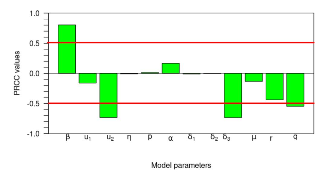
Figure 3: Tornado plot for the global sensitivity analysis of parameters within R0.
while parameters u2, δ3, r, and q have negative PRCC values since the PRCC values are strictly greater than ±0.2. Therefore, the biological implications of an increased transmission rate implies that an increase in the number of infected TB infections, while an increase in u2, δ3, r, and q leads to a decrease in the
Table 2: Table of PRCC values for all model parameters in \(\mathcal{R}_0\). The larger PRCC values are indicated with *, implying that these corresponding parameters are more significant.
| Parameters | PRCC value: \(\mathcal{R}_0\) | P-value | Keep? |
|---|---|---|---|
| β | 0.803812255* | \(0.000000e^{00}\) | TRUE |
| \(u_1\) | -0.162104365 | \(4.824347e^{-07}\) | TRUE |
| \(u_2\) | -0.731077708* | \(0.000000e^{00}\) | TRUE |
| \(\eta\) | -0.007917008 | \(8.767275e^{-01}\) | FALSE |
| p | 0.014487159 | \(8.655386e^{-01}\) | FALSE |
| \(\alpha\) | 0.166551573 | \(2.597758e^{-07}\) | TRUE |
| \(\delta_1\) | -0.011134247 | \(8.719335e^{-01}\) | FALSE |
| \(\delta_2\) | -0.002306109 | \(9.422729e^{-01}\) | FALSE |
| \(\delta_3\) | \(-0.733021841^*\) | \(0.000000e^{+00}\) | TRUE |
| \(\mu\) | -0.134391857 | \(3.269048e^{-05}\) | TRUE |
| r | \(-0.438655427^*\) | \(0.000000e^{+00}\) | TRUE |
| q | \(-0.546904569^*\) | \(0.000000e^{+00}\) | TRUE |
infection dynamics of TB. Hence, we aimed to implement control measures required to reduce the infection rate to reduce the risk of transmission or the infected population, which are I and \(R_1\)-individuals. Table 2 shows that the parameters \(\beta\), \(u_1\), \(u_2\), \(\alpha\), \(\delta_3\), \(\mu\), r, and q have p-values less than 0.05, which indicates that they have a significant effect on the reproduction number and consequently on the transmission dynamics of the model. Hence, we targeted to establish control measures that could reduce the transmission rate, \(\beta\), and promote the increase of \(u_1\), \(u_2\), \(\alpha\), \(\delta_3\), \(\mu\), r, and q. See the following literature [53], [54], [56], [55], where a similar sensitivity analysis has also been presented to ascertain the model parameter that causes the disease to spread or affect the basic reproduction number for other epidemic models in the human population.
6.2. Dependency of the endemic level and control reproduction number to the model parameters
Next, we examined the impact of intervention parameters, namely case detection rate \((u_1)\) and the probability of success of second dose treatment \((u_2)\) on the size of the control reproduction number and the size of active TB compartment on the endemic equilibrium. We began by determining the derivative of \(\mathcal{R}_0\) respect to \(u_1\), which gave us the following:
\[\frac{\partial \mathcal{R}_0}{\partial u_1} = -\beta \frac{(\eta(\mu + u_2 \delta_3) + \delta_2(1 - q))(1 - p)(\alpha(r\delta_1 + \mu) - \mu\delta_1(1 - r))}{(\mu + \delta_2)(\mu + \delta_1)(u_2 \delta_3 + \mu)(u_1 + \alpha + \mu)^2}.\]
It can be seen that \(\frac{\partial \mathcal{R}_0}{\partial u_1}\) can be either positive or negative. It makes sense that we aimed to reduce the control reduction number by increasing the case detection rate. However, this is not always the case. The control reproduction number may increase when the case detection rate increases. To analyze this further, we examined the effect of case detection \((u_1)\) and the quality of first dose treatment (r) on \(\frac{\partial \mathcal{R}_0}{\partial u_1}\). It is easy to calculate that \(\frac{\partial \mathcal{R}_0}{\partial u_1} < 0\) if and only if
\[r > r^* = \frac{\mu(\delta_1 - \alpha)}{\delta_1(\alpha + \mu)}.\]
Since r is a proportion, which is always non-negative, if \(\alpha > \delta_1\), then we will always have \(\frac{\partial \mathcal{R}_0}{\partial u_1} < 0\) for all possible value r. Hence, whenever the progression rate of latent undetected individuals is higher than the recovery rate of detected latent individuals (\(\delta_1 < \alpha\)), increasing case detection will always succeed in reducing \(\mathcal{R}_0\). However, if \(\delta_1 > \alpha\), then there is a minimum level of probability of success for the first dose treatment such that increasing case detection could reduce \(\mathcal{R}_0\). For a numerical experiment, we substituted all parameter values in Table 1 except \(u_1\) and r, which gave the following:
\[\frac{\partial \mathcal{R}_0}{\partial u_1} = -\frac{81.667(0.527r - 0.001)}{(u_1 + 0.303)^2}.\]
We have that \(\frac{\partial \mathcal{R}_0}{\partial u_1} < 0\) if r > 0.0074. If the quality of the first dose treatment is low (for example, less than 0.0074), then increasing case detection will only increase \(\mathcal{R}_0\). Hence, the quality of treatment should pass this threshold (for example, \(r > r^* = 0.0074\)) such that improving case detection causes a reduction of \(\mathcal{R}_0\) whenever the case detection rate is increased.
To provide a clearer understanding of the findings above, readers can refer to the illustration in Figure 4. We use all the same parameters as in Table 1. Figure 4(a) shows how \(\frac{\partial \mathcal{R}_0}{\partial u_1}\) changes depending on the value of r. It can be seen that if \(r=0.005 < r^*\), then \(\frac{\partial \mathcal{R}_0}{\partial u_1}\) is always positive. As a result, increasing the control value u1 will always increase \(\mathcal{R}_0\). This is certainly counterproductive to the vision of increasing case detection, which aims to reduce the value of the basic reproduction number. Conversely, if \(r=0.1>r^*\), then increasing the value of u1 will decrease \(\mathcal{R}_0\). This is in line with the expectation that increasing case detection will suppress the basic reproduction number.
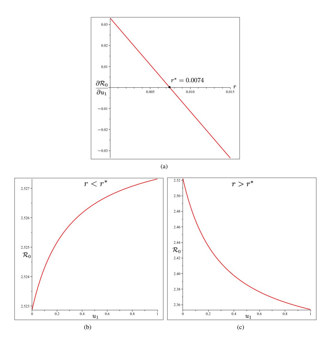
Figure 4: Effect of r on \(\frac{\partial \mathcal{R}_0}{\partial u_1}\) (panel a). Using specific value of r we show the effect of \(u_1\) on \(\mathcal{R}_0\) when \(r < r^*\) (panel b) and when \(r > r^*\) (panel c). All parameter used is given in Table 1.
The derivation of \(\mathcal{R}_0\) respect to the probability of success of the second dose treatment \((u_2)\) is given by
\[\frac{\partial \mathcal{R}_{0}}{\partial u_{2}} = -\frac{\delta_{3} \left( pr \delta_{1} u_{1} + \mu^{2} p + \mu p \delta_{1} + \mu p u_{1} + (1 - r) \delta_{1} u_{1} + \alpha \mu + \alpha \delta_{1} \right) \beta \left( 1 - q \right) \delta_{2}}{\left( \mu + \delta_{2} \right) \left( \mu + \delta_{1} \right) \left( u_{2} \delta_{3} + \mu \right)^{2} \left( u_{1} + \alpha + \mu \right)},\]
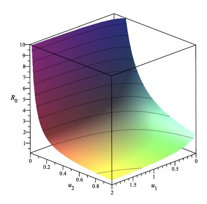
Figure 5: Dependency of \(\mathcal{R}_0\) respect to case detection rate \((u_1)\) and probability of success of the second dose treatment.
which is always negative. Hence, improving the quality of the second dose treatment is essential to reduce \(\mathcal{R}_0\). To see the impact of \(u_1\) and \(u_2\) to \(\mathcal{R}_0\), we set the parameter values as given in Table 1, but left \(u_1\) and \(u_2\) free. Substituting these parameter values and applying it on \(\mathcal{R}_0\), we have:
\[\mathcal{R}_0(u_1, u_2) = \frac{2.802(0.018u_2 + 0.108)(0.133u_1 + 0.255)}{(0.158u_2 + .003)(u_1 + 0.303)}.\]
The plot of \(\mathcal{R}_0(u_1,u_2)\) is given in Figure 5. It can be seen that since r>r*=0.0074, increasing case detection and the probability of success of the second dose treatment can reduce the size of the control reproduction number significantly. Another interesting result is given in Figure 6, which presents the impact of case detection rate and probability of success of the second dose treatment on the size of the total active TB in the endemic equilibrium point. It can be seen that a higher case detection rate could reduce the number of active TB at the equilibrium point level. However, an increased probability of success of the second dose treatment does not always translate to a reduction in the endemic level of active TB. For a relatively small \(u_2\) in Figure 6, we can see that \(\frac{\partial I^*}{\partial u_2} > 0\). Hence, increasing \(u_2\) in this interval is counterproductive to the TB control intervention since it will increase the number of I at the endemic equilibrium point. When \(u_2\) larger enough, the positive impact of \(u_2\) start to appear, since \(\frac{\partial I^*}{\partial u_2} < 0\) in this interval. The number of I in the endemic equilibrium decreases as \(u_2\) increases until it reaches its critical point where \(\mathcal{R}_0 = 1\), where we have no more I at the equilibrium point.
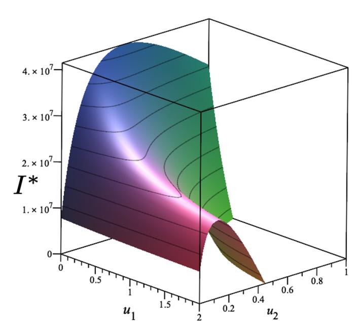
Figure 6: Dependency of the endemic size of \(I^*\) respect to the treatment rate \((u_1)\) and probability of success of second dose treatment \((u_2)\).
The results given in Figure 5 are relevant to the result shown in Figure 7. Figure 7 shows the impact of case detection rate on the magnitude of \(\mathcal{R}_0\) and the size of endemic equilibrium of the active infected individual compartment \((I^*)\), which is given by EE (6). It can be seen that increasing the case detection rate could reduce \(\mathcal{R}_0\) as well as the equilibrium size of the active TB compartment. In the example in Figure 7, we have that \(\mathcal{R}_0 < 1\) if \(u_1 > 0.768\). As a consequence, based on Theorem 3, there is no endemic equilibrium when \(u_1 > 0.768\). An autonomous simulation on the impact of case detection rate can be seen in Figure 8. It can be seen that the number of undetected and detected latent TB, active TB, and imperfect recovered TB could be reduced with a higher rate of case detection. Furthermore, if \(u_1 > 0.768\), the dynamics of infected compartments tend to 0. The larger the case detection rate, the faster the dynamics tend toward the TB-free equilibrium.
In the following simulation, we analyze the impact of the success probability of the second dose treatment on the size of endemic equilibrium and the dynamic of active TB-infected individuals. As we already depicted in Figure 6, the impact of \(u_2\) only succeeds sometimes in reducing the number of I at the endemic equilibrium point. For more details with a fixed value of \(u_1\), the impact of \(u_2\) on the size of I at the endemic equilibrium point can be seen in Figure 9. It can be noted that increasing \(u_2\) will reduce \(\mathcal{R}_0\). However, increasing \(u_2\) does not always give a positive result in the reduction of I at the endemic equilibrium point. Figure 9 indicates that \(I^*\) is monotonically increasing when \(u_2 < 0.151\), and its turning point is at \(u_2 = 0.151\). When \(u_2 > 0.151\), as can be seen, increasing \(u_2\) will reduce the size of I at its endemic equilibrium point. Although the number of I at the endemic equilibrium point in some intervals of \(u_2\) could be increased, the total number of active TB individuals is always reduced when \(u_2\) increases, as shown in Figure 10.
To visualize the impact of \(u_2\) when it is less than or larger than its critical value (turning point), we run several values of \(u_2\) to see the dynamic of each infected compartment of our system (2). Figure 11 shows how the dynamic of each compartment behaves for many values of \(u_2 < u_2^*\), where \(u_2^*\) is the turning point of \(u_2\); see Figure 9. In this case, \(u_2^* = 0.151\). We can see that for a long-term simulation, a larger value of \(u_2\), where \(u_2 < 0.151\), will increase \(E_1, E_2\),, and I but reduce the size of \(R_1\). On the other hand, when \(u_2 > 0.151\), as shown in Figure 12, then a larger value of \(u_2\) will increase the number of \(E_1, E_2, I\),, and \(R_1\) reach the disease-free equilibrium faster.
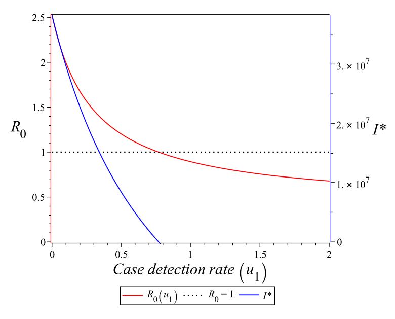
Figure 7: Dependency of R0 and endemic size of I ∗ respect to case detection rate (u1).
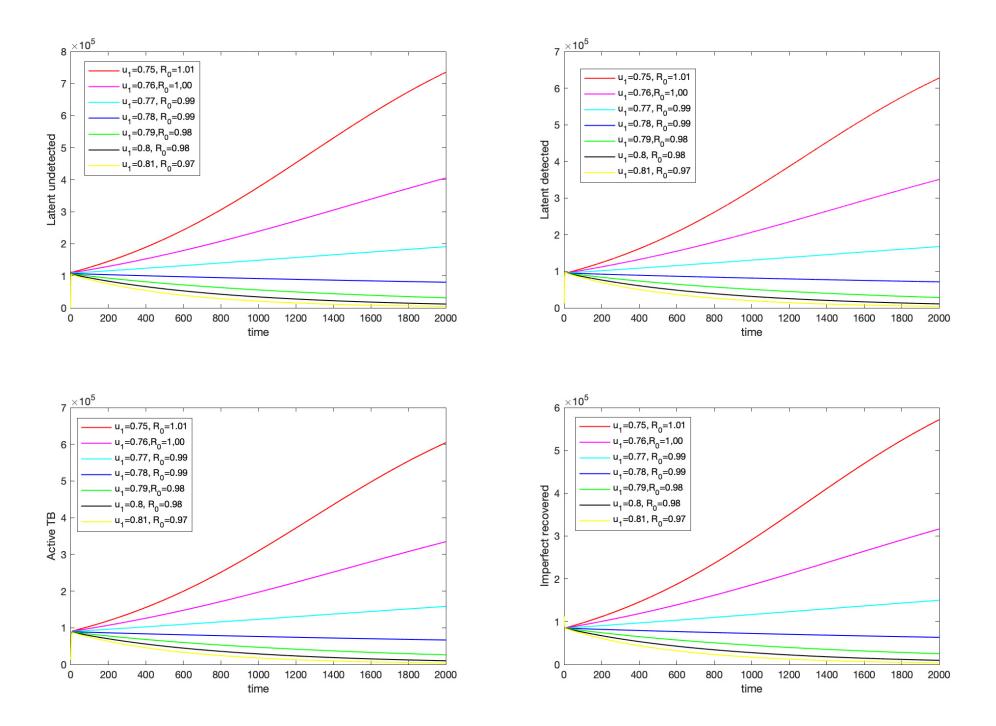
Figure 8: Dynamic of all infected compartments for various values of case detection rate (u1).
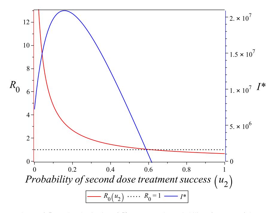
Figure 9: Dependency of R0 and endemic size of I ∗ respect to the probability of success of the second dose of treatment (u2).
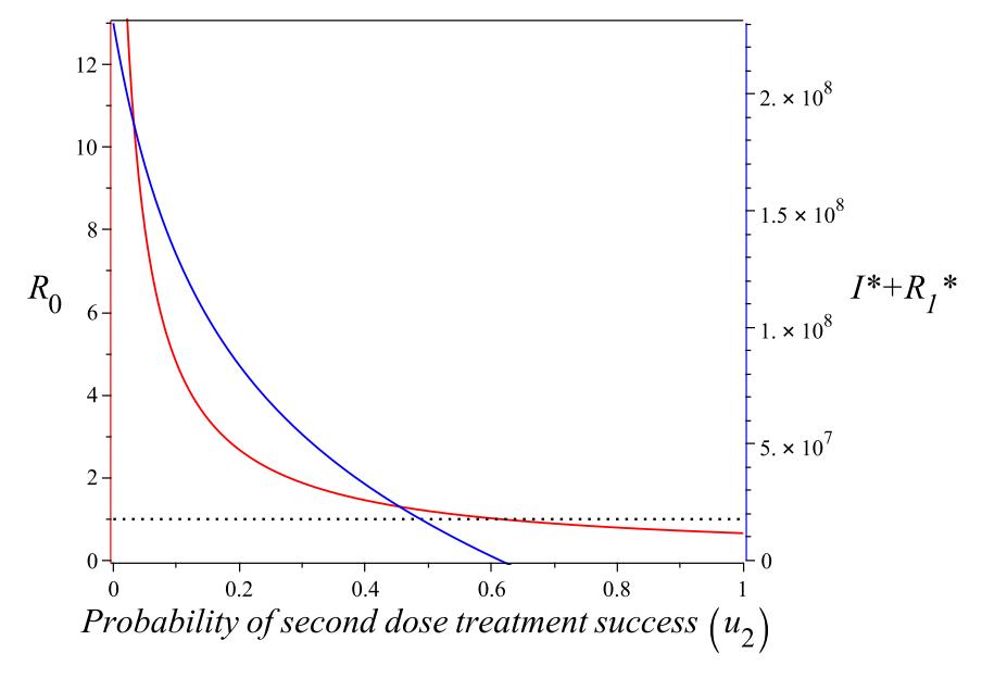
Figure 10: Dependency of R0 and endemic size of I ∗ + R ∗ 1 respect to the probability of success of the second dose of treatment (u2).
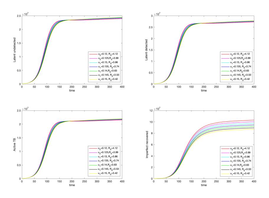
Figure 11: Dynamic of all infected compartments for various values of u2 less than the critical u2.
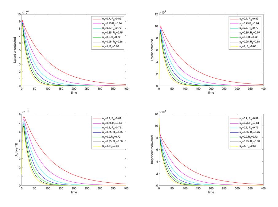
Figure 12: Dynamic of all infected compartments for various values of u2 larger than the critical u2.
7. CONCLUSION
TB is a contagious disease that has become a significant health problem in many countries, including Indonesia, which reported more than 9% of the world's TB cases in 2021 [3]. Various interventions have been implemented by the government and WHO to handle the spread of TB, including mass campaigns, vaccination, treatment, and many more [57], [58]. Many recent reports state that early case detection of TB cases could be an effective strategy for handling the spread of TB. This intervention aims to give early treatment for the latent TB-infected individual as soon as possible such that they can be cured faster before they can spread TB to others. Another critical factor in TB transmission is that TB treatment has a significant potential for failure if the treated individual does not observe discipline in following the treatment. Unlike previous studies presenting TB mathematical models [59], [29], this article aimed to understand the impact of early case detection and treatment failure on TB control programs. The model was constructed as a system of nonlinear ordinary differential equations as shown in model (2), dividing the human population based on their health and treatment status as susceptible individuals, individuals with detected and undetected latent TB, active TB individuals, and imperfectly and perfectly recovered individuals. It has been proved in Propositions 1 and 2 that the proposed model always has a non-negative solution for all non-negative initial conditions. This property is vital since our solutions describe the number of individuals, which has a biological interpretation only when they are non-negative.
Mathematical analysis of the proposed model included the existence of the equilibrium points, the control reproduction number, local and global stability of the TB-free equilibrium, bifurcation analysis, and sensitivity analysis. We find that the TB-free equilibrium is globally asymptotically stable if R0 < 1. Furthermore, we discovered that the TB-endemic equilibrium only exists if R0 > 1. The bifurcation analysis using the Castillo– Song bifurcation theorem [48] showed that the model only could exhibit a forward bifurcation at R0 = 1. Unlike other TB transmission models [60], [61], backward bifurcation phenomena do not appear in this model. Hence, controlling the size of the control reproduction number is essential to finding the best strategy to prevent the spread of TB among the population. We used accumulated data on TB cases in Indonesia from 2017 to 2021 to find the best-fit parameters for our model. These parameters were used in sensitivity analysis and autonomous simulations. Sensitivity analysis was conducted in this study to understand the most significant parameters that can be used to control the control reproduction number. With a combination of the Latin hypercube sampling (LHS) method and the partial rank correlation coefficient (PRCC), we found that the infection parameter is the most dominant one that can affect the control reproduction number. The larger the infection parameter, the larger the control reproduction number. Furthermore, we discovered that increasing the probability of success of the second dose treatment is more significant in reducing the control reproduction number compared with the case detection rate. Our sensitivity analysis of u2 showed that increasing u2 could increase the endemic size of the active TB compartment if the implementation of u2 is smaller than its critical value. Hence, the quality of the second dose treatment should be good enough to prevent the increase of active TB cases in the population.
As with any mathematical modeling framework, we acknowledge that simplifications and assumptions in our model may lead to various limitations on its applicability and implementation. Some of the limitations in our model include that we did not consider possible phenomena of multi-drug resistance (MDR-TB), relapse, or co-infection with other diseases such as HIV or COVID-19. Despite these limitations, we maintain that our model is applicable in real-life scenarios in any community induced by tuberculosis disease. Therefore, future research can be done by incorporating the listed limitation, which can help to improve our model.
ACKNOWLEDGEMENTS
The authors would like to acknowledge the anonymous editor and reviewers. This research is funded by Directorate of Research and Development, Universitas Indonesia with PUTI Q2 research grant scheme 2023 (ID number NKB-759/UN2.RST/HKP.05.00/2023).