

1. Introduction
Cancer is characterized by out-of-control cell growth and tissue invasion. It is one of the leading causes of death globally. According to the World Health Organization (WHO), there were an estimated 19.3 million cases in 2020. This number is projected to rise to 28.4 million cases by 2040 [32]. The majority of cancer cases occur in developed countries such as the USA and Europe [23]. There are numerous types of cancer, including prostate, stomach, colorectal, lung, melanoma, breast, uterine, liver, bladder, kidney, and many other types. Among these, the most common types are lung, breast, colon, melanoma, stomach, and prostate cancers [23], [26].
Cancer can be classified into a group of diseases that begin when normal cells transform into cancerous cells, also known as tumor cells. These cancerous cells have the ability to multiply and spread. However, as cancerous cells develop and proliferate within the body, the immune system identifies them as abnormal and potentially hazardous, mobilizing to eliminate them from the host organism.
1.1. The immune system
The immune system consists of specialized types of cells and molecules whose function is to protect the host against infection. These components are divided into two main categories: innate (or natural) and acquired (or adaptive), according to their operational mechanisms and time of response to the infections.
When it comes to combating tumor cell proliferation, a particular set of immune cells known as tumor-infiltrating cytotoxic lymphocytes (TICLs), plays a crucial role. These TICLs represent a distinct subset of immune cells that target and destroy cancer cells. They include components from both the innate and adaptive immune systems. Moreover, this group includes CD8<sup>+</sup> T lymphocytes (CD8<sup>+</sup> T cells), CD4<sup>+</sup> T lymphocytes (CD4<sup>+</sup> T cells), natural killer (NK) cells, B lymphocytes (B cells), and several other relevant cell types.
*Corresponding author
Received October \(27^{th}\), 2023, Revised March \(4^{th}\), 2024 (first), Revised June \(18^{th}\), 2024 (second), Accepted for publication June \(27^{th}\), 2024. Copyright ©2024 Published by Indonesian Biomathematical Society, e-ISSN: 2549-2896, DOI:10.5614/cbms.2024.7.1.7
1.2. Dynamics of converting normal cells into tumor cells
Normal cells convert into tumor cells when gene mutations occur, a process clearly observed in many types of cancer, such as breast cancer, known for its genetic mutations [38]. Furthermore, studies have demonstrated that the cytokine transforming growth factor-beta (TGF-β) can initiate the conversion of normal cells into tumor cells, playing a significant role in cancer onset. For instance, Roberts et al. [37] demonstrated that TGF-β can induce malignant behavior in normal fibroblasts, enabling them to acquire malignant properties and become cancerous.
It is well-established that normal cells, platelets, osteoblasts, and other bone cells are major sources of TGF-β secretion. Additionally, activated immune cells such as lymphocytes, macrophages, and neutrophils are also known to secrete TGF-β. Moreover, tumors and tumor cell lines contribute to the production of TGF-β [12].
However, while TGF-β suppresses cancer in the early stages of tumorigenesis by inhibiting cell proliferation and promoting cell death, it can paradoxically promote cancer in advanced stages. At these later stages, TGFβ facilitates cancer progression by stimulating tumor angiogenesis, progression, and metastasis. It promotes tumor angiogenesis, aiding in the formation of new blood vessels to support tumor growth [39]. Additionally, TGF-β enhances the growth and metastasis of tumor cells by inducing a mesenchymal transition in epithelial cells. This process results in epithelial cells losing their characteristics and acquiring mesenchymal-like properties, making cancer cells more motile and capable of migrating and invading surrounding tissues from their primary site [40].
1.3. Cancer treatments
Cancer treatment can be categorized into surgery, radiotherapy, chemotherapy, small interfering RNA (siRNA), and other hospitalizations [4], [34]. Various methods can be employed for treating cancer, and at times, a combination of two or more treatments is necessary, such as chemotherapy and radiation, surgery and radiation therapy, or surgery and chemotherapy [16], [17], [24]. Here, we focus on chemotherapy and siRNA as primary therapeutic approaches for cancer treatment.
Chemotherapy stands out as one of the most effective and widely used treatments for diverse types of cancer, including anal, bladder, breast, and gastroesophageal cancer. While chemotherapy yields positive effects on tumor cells, it also causes side effects impacting the skin, hair, bone marrow, blood, gastrointestinal tract, kidneys, heart, lungs, and brain. These side effects arise from the fact that chemotherapy not only targets cancer cells but also affects normal and immune cells [3], [7], [30].
Another method in cancer treatment involves the use of siRNA. SiRNA finds application in treating various diseases and cancer types [5], [21], though challenges persist in achieving effective delivery to the cancer site [21]. In cancer treatments, siRNA is designed to directly target and silence specific genes involved in cancer growth and proliferation through enzymatic cleavage of target mRNA [2], [22], [31]. Additionally, siRNA can effectively suppress the activity of TGF-β expression in tumors by targeting its mRNA molecules [47], [1], resulting in reduced invasiveness of cancer cells.
While siRNA is generally considered less toxic compared to chemotherapy [46], it is not without side effects. One possible side effect is the off-target effect, where siRNA delivery may not accurately reach its intended target cells, leading to the unintended suppression of genes in other cell types [21]. Moreover, siRNA may induce an inflammatory response by activating immune cells that recognize siRNA as foreign [46].
1.4. Mathematical models of tumor-immune interaction dynamics
Over the past few decades, several mathematical models such as those in [10], [11], [18], [20], [25] and more recently [36], have been developed to understand the mechanisms and dynamics of tumor growth and their interactions with the immune system. De Pillis et al. [10] presented a model describing the competition between cancer cells, normal cells, immune cells, and chemotherapy. They qualitatively simulated the asynchronous tumor-drug interaction known as "Jeff's phenomenon." The model successfully captured the behavior of asynchronous response. In their subsequent work [11], they developed another model describing the interaction between the same cell types. They investigated pulsed therapy and optimal control therapy to determine how each treatment can lead to a desirable basin of attraction. Their findings show that optimal control therapy successfully drives the system into a desirable basin of attraction, whereas pulsed chemotherapy does not.
Itika et al. [18] discussed the interaction between tumor and immune cells, and they used linear time-varying (LTV) optimal control to investigate the dynamical evolution of tumor cells in a tumor environment. Their study demonstrated a significant reduction in the number of tumor cells with a small dose of chemotherapy and a short duration of treatment. Ku-Carrilloa et al. [20] developed a simple tumor model along with normal and immune cells. Their model focused more on the relationship between cancer and obesity, which investigates the negative effects of obesity on cancer and the effects of a low or high-caloric diet. Their findings revealed that a low-calorie diet has a therapeutic effect, which can be used as an adjuvant in anticancer treatment. Oke et al. [25] developed a model of interaction between tumor, normal, and immune cells. Additionally, their model includes estrogen as a tumor promoter. To effectively eliminate tumor cells, the researchers employed a combination of chemotherapy and ketogenic diet treatments while utilizing optimal control techniques for treatment administration.
Furthermore, cytokines play a crucial role in tumor-immune cell communication and are often integrated into mathematical models that study these interactions. Numerous mathematical models, encompassing both earlier works cited in [1], [8], [19], [35], and more recent contributions by [15], [33], [36], have been developed to illustrate the dynamics of tumor cell growth, the immune system response, and the role of cytokines, which can either enhance immune responses or promote tumor progression.
Kirschner et al. [19] incorporated the cytokine interleukin-2 (IL-2) into their model to enhance the resistance of immune cells and aid in the elimination of tumor cells. Their study findings indicated that IL-2 by itself is not effective in eradicating tumors. However, promising outcomes in cancer eradication were observed when IL-2 was used in combination with adoptive cellular immunotherapy. Arciero et al. Arciero et al. [1] extended the work done by Kirschner et al. [19] by incorporating TGF-β and siRNA treatment, where TGF-β promotes tumor growth, while siRNA suppresses TGF-β production. Their study showed that siRNA alone is not capable of eradicating tumor cells from the body; rather, it reduces their size. Other studies, such as [8], [35], have also incorporated various cytokines into their mathematical models to enhance the immune response against cancer cells.
In this study, we first analyze the dynamics of tumor growth promoted by the cytokine TGF-β and examine the response of the immune system in the absence of any treatment effects. Secondly, in the optimal control section, we investigate the effects of chemotherapy and siRNA. Chemotherapy is employed to inhibit the growth of cancer cells, while siRNA technology targets TGF-β, which converts normal cells into tumor cells. Specifically, siRNA was employed to effectively suppress the activity of TGF-β by targeting its mRNA molecules [47], [1].
We chose the combination of chemotherapy and siRNA for tumor treatment due to their numerous advantages. Chemotherapy remains one of the top selections for cancer treatment for many considerations, including its ability to target and destroy cancer cells. It can be effectively combined with other treatments, such as surgery, radiotherapy, or immunotherapy, and improve survival rates. Additionally, chemotherapy can shrink tumors, alleviating symptoms and improving life quality in advanced-stage cancers where cancer is not possible to treat [41], [42].
On the other hand, siRNA presents a promising approach for cancer treatment due to its ability to target and silence oncogenes or genes responsible for tumor growth and enhance sensitivity to chemotherapy. Silencing these oncogenes reduces tumor cells' resistance to chemotherapy. Furthermore, siRNA plays a crucial role in helping stop metastasis by suppressing the activity of TGF-β in the tumor [43], [44], [47].
This paper is structured as follows. In Section (2), we briefly describe how our model is obtained and what assumptions are made. In Section (3), we discuss the positivity and boundedness of the solutions in our model. Additionally, we discuss reducing the number of parameters in the model using the non-dimensionalization technique. Finally, we explore the existence of equilibria and their stability in both tumor-free and coexistence cases. Section (4) presents the numerical simulations of the system without treatment (without control). In Section (5), optimal control strategies are formulated. Additionally, we present the numerical simulations for the optimal control and its discussion. In Section (6), we summarize and present our conclusion.
2. MODEL FORMULATION
In this section, we introduce a new mathematical model that describes the interactions among tumor cells, normal cells, immune cells, and TGF-\(\beta\). The cell populations and cytokine concentration at time t are denoted as follows:
- T(t), the population of tumor cells,
- N(t), the population of normal cells,
- I(t), the population of immune cells,
- K(t), the concentration of TGF-\(\beta\).
To model the interactions between these populations, we propose a system of ordinary differential equations, represented as follows:
\[\frac{dT}{dt} = \alpha_T T - d_T T - \alpha_c I T + \beta_K K N, \frac{dN}{dt} = \alpha_N N \left( 1 - \frac{N}{N_{Max}} \right) - d_N N - \xi_N K N, \frac{dI}{dt} = s + \frac{pIT}{q+T} - d_I I, \frac{dK}{dt} = \alpha_K T - d_K K,\] (1)
with non-negative initial conditions \(T(0) = T_0\), \(N(0) = N_0\), \(I(0) = I_0\), and \(K(0) = K_0\).
In the system (1), the first equation describes the dynamics of tumor cells, which are assumed to grow exponentially, as indicated by the term \(\alpha_T T\), where \(\alpha_T\) represents the growth rate. This type of exponential growth has been confirmed in various cancer types, including breast cancer [55] and lung cancer [56]. The natural death of tumor cells is given by the term \(d_T T\), where \(d_T\) represents the death rate. This natural death results from a lack of nutrients and oxygen. We assume that tumor cells are killed by TICLs, represented by the term \(\alpha_c IT\), where \(\alpha_c\) denotes the killing rate. Additionally, the term \(\beta_K KN\) represents the increase in the tumor population through the conversion of normal cells into tumor cells due to their interactions with TGF-\(\beta\). Converted normal cells will now form the class of tumor cells, and therefore, the tumor cell population will increase at a rate \(\beta_K\), resulting in a growth factor of \(\beta_K KN\) on the tumor cell population.
The dynamics of normal cells are described by the second equation of the system (1). Normal cells are assumed to grow logistically, as described by the term \(\alpha_N N(1-\frac{N}{N_{Max}})\), where \(\alpha_N\) represents the growth rate and \(N_{Max}\) represents the maximum carrying capacity. The term \(d_N N\) denotes the natural death of normal cells, with \(d_N\) representing the death rate. This natural death results from competition for resources such as nutrients and oxygen or from the accumulation of substances released from cell metabolism within the cells themselves. TGF-\(\beta\) is assumed to prompt the conversion of normal cells into tumor cells, represented by the term \(\xi_N K N\), where \(\xi_N\) denotes the conversion rate (or rate of tumor formation).
The third equation of the system (1) describes the dynamics of immune cells (TICLs). TICLs are assumed to have a constant source rate, s. Additionally, TICLs are recruited in response to the presence of tumor cells, with this recruitment given by the Michaelis-Menten term \(\frac{pIT}{q+T}\), where p represents the maximum recruitment rate, and q is the Michaelis-Menten constant, representing the concentration of tumor antigens required to achieve half-maximal activation of TICLs. The term \(d_II\) denotes the natural death of immune cells, with \(d_I\) representing the death rate.
The final equation of the system (1) represents the kinetics of TGF-\(\beta\) production. Malignant tumor cells are assumed to produce TGF-\(\beta\). This production is represented by the term \(\alpha_K T\), where \(\alpha_K\) represents the production rate. The term \(d_K K\) represents the decay of TGF-\(\beta\), where \(d_K\) represents the decay rate.
The parameter values in model (1) were collected from published literature and experimental data, and they are given in Table 1. However, longitudinal data for parameters governing interactions between normal cells and TGF-\(\beta\) are not available. Therefore, we made assumptions that are consistent with our model.
| Parameter | Description | Estimated value | Units | Source | |
|---|---|---|---|---|---|
| \(\alpha_T\) | Tumor cells growth rate | 1.5 | day 1 | [11] | |
| \(d_T\) | Tumor cells death rate | \(1 \times 10^{-6}\) | day 1 | [53] | |
| \(\alpha_c\) | Killing rate of tumor cells by immune cells | \(1 \times 10^{-2}\) | cell 1 | [51] | |
| \(\beta_K\) | Rate of tumor cell growth from the converted normal cells | 0.5 | cell.day 1 | Assumed | |
| \(\alpha_N\) | Normal cells growth rate | 1 | day 1 | [11] | |
| \(N_{Max}\) | Normal cells carrying capacity | \(3 \times 10^{5}\) | cell 1 | Assumed | |
| \(d_N\) | Normal cells death rate | 0.29 | day 1 | Assumed | |
| \(\xi_N\) | Conversion rate of normal cells into tumor cells | \(1 \times 10^{-12}\) | day 1 | Assumed | |
| s | Constant source of immune cells | \(1.3 \times 10^{4}\) | cells 1 | [10], [25] | |
| \(d_I\) | Immune cells death rate | 0.2 | day 1 | [11] | |
| p | Maximum immune cells recruitment rate by tumor cells | 0.2 | cell.day 1 | [14], [25] | |
| q | Half-saturation constant of tumor antigens | \(3 \times 10^{5}\) | cell | [25], [27] | |
| \(\alpha_K\) | Production rate of TGF-\(\beta\) by tumor cells | \(2 \times 10^{-4}\) | IU.day - 1 | [1] | |
| \(d_K\) | decay rate of TGF-\(\beta\) | \(7 \times 10^{-3}\) | IU.day 1 | [52] | |
| \(C_T\) | Killing rate of tumor cells by chemotherapy | 0.8 | pg.day 1 | [9], [13] | |
| \(C_N\) | Killing rate of normal cells by chemotherapy | 0.6 | pg.day 1 | [9], [13] | |
| \(C_I\) | Killing rate of immune cells by chemotherapy | 0.6 | pg.day 1 | [9], [13] | |
Table 1: Parameter definitions, values, and their sources for model system (1).
3. MODEL ANALYSIS
In this section, we discuss the positivity and boundedness of solutions. Additionally, we conduct a qualitative analysis to establish the long-term behavior of the system.
3.1. Model well-posedness
In this subsection, we show that the solutions of the model system (1) have biological meaning. In order to show that, it is required to prove that the solutions of the system are both positive and bounded for all time.
Theorem 3.1 (Positivity). Given positive initial conditions T(0), N(0), I(0), K(0), then the solutions T(t), N(t), I(t), K(t) of the model system (1) will always be non-negative.
Proof: Since all the parameters used in the model system (1) are positive, we obtain the following inequality from the first equation of the model system (1)
\[\frac{dT}{dt} = \alpha_T T - d_T T - \alpha_c IT + \beta_K KN \ge -d_T T - \alpha_c IT,\] by separating variables and integrating both sides, we get:
\[T(t) \geq T(0)e^{-\int_0^t \left(d_T + \alpha_c I(t)\right)dt}\] this proves that \(T(t) \ge 0\) for all t > 0.
Similarly, from the second, third, and fourth equations in the model system (1), we have
\[N(t) \ \geq \ N(0)e^{-\int_0^t \Big(d_N \, + \, \xi_N K(t)\Big) dt} \ , \ I(t) \ \geq \ I(0)e^{-d_I t}, \ \text{and} \ K(t) \ \geq \ K(0)e^{-d_K t}.\]
This proves that all the solutions of model system (1) are positive.
Theorem 3.2 (Boundedness). Assume that the following condition holds:
\[d_I > \lambda_I\], then, all solutions T(t), N(t), I(t), K(t) of model system (1) with positive initial conditions \(T_0\), \(N_0\), \(I_0\), \(I_0\), are bounded in the region
\[\Delta = \left\{ (T, N, I, K) \in \mathbb{R}_+^4 : T(t) \le \frac{\lambda_T}{d_T}, N(t) \le N_{Max}, I(t) \le \frac{s}{d_I - \lambda_I}, K(t) \le \frac{\lambda_K}{d_K} \right\}.\]
Proof: From the second equation of the model system (1), we have
\[\frac{dN}{dt} \le \alpha_N N \left( 1 - \frac{N}{N_{Max}} \right) \le \alpha_N N - \lambda_N N^2, \tag{2}\] where
\[\lambda_N = \frac{\alpha_N}{N_{Max}},\] by using Bernoulli's method, we have
\[N \le \frac{\alpha_N}{\lambda_N + C\alpha_N e^{-\alpha_N t}},\] where
\[C = \frac{\alpha_N - N_0 \lambda_N}{\alpha_N N_0},\] and
\[N_0 = \frac{\alpha_N}{\lambda_N + C\alpha_N}.\]
Consequently,
\[N \le \frac{\alpha_N}{\lambda_N + \frac{\alpha_N - N_0 \lambda_N}{N_0} e^{-\alpha_N t}},\]
\[\lim_{t\to\infty}\sup\,N(t)\ \le\ \frac{\alpha_N}{\lambda_N}\le N_{Max},\] this proves that N(t) is bounded.
Similarly, respectively, from the first, fourth, and third equations of the model system (1), we have
\[\frac{dT}{dt} \le \lambda_T - d_T T,\] where λT = αN βKK λN . By integrating both sides, we have
\[T \le \frac{\lambda_T}{d_T} + T_0 e^{-d_T t}\]
\[\lim_{t\to\infty} \sup T(t) \ \le \ \frac{\lambda_T}{d_T}.\]
\[\frac{dK}{dt} \le \lambda_K - d_K K,\] where λK = αKλT dT .
\[K \le \frac{\lambda_K}{d_K} + K_0 e^{-d_K t},\]
\[\lim_{t\to\infty}\sup K(t) \ \le \ \frac{\lambda_K}{d_K}.\]
\[\frac{dI}{dt} \le s + (\lambda_I - d_I)I \le s - (d_I - \lambda_I),\] where \(\lambda_I = \frac{\lambda_T}{qd_T + \lambda_T}\).
\[I \le \frac{s}{d_I - \lambda_I} + I_0 e^{-(d_I - \lambda_I)t},\]
\[\lim_{t \to \infty} \sup I(t) \le \frac{s}{d_I - \lambda_I}.\]
Therefore, the solutions of model system (1) are bounded.
3.2. Non-dimensionalization
To simplify the analysis of our system (1), we begin by re-scaling the system equations using the following substitutions:
\[T = \hat{T}\bar{T}, \quad N = \hat{N}\bar{N}, \quad I = \hat{I}\bar{I}, \quad K = \hat{K}\bar{K}, \quad \text{and} \quad t = \hat{t}\bar{t}.\] (3)
The non-dimensionalized system can be written as follows:
\[\frac{d\bar{T}}{d\bar{t}} = \bar{T} - \phi_1 \bar{T} - \phi_2 \bar{I}\bar{T} + \phi_3 \bar{K}\bar{N},\] \[\frac{d\bar{N}}{d\bar{t}} = \psi_1 \bar{N} \left( 1 - \bar{N} \right) - \psi_2 \bar{N} - \psi_3 \bar{K}\bar{N},\] \[\frac{d\bar{I}}{d\bar{t}} = 1 - \delta_1 \bar{I} + \frac{\delta_2 \bar{I}\bar{T}}{\delta_3 + \bar{T}},\] \[\frac{d\bar{K}}{d\bar{t}} = \bar{T} - \chi \bar{K},\] (4)
with non-negative initial conditions \(\bar{T}(0)=\bar{T}_0, \ \bar{N}(0)=\bar{N}_0, \ \bar{I}(0)=\bar{I}_0, \ \text{and} \ \bar{K}(0)=\bar{K}_0.\) Where
\[\begin{split} \hat{t} &= \frac{1}{\alpha_T} \quad , & \hat{T} &= \frac{\beta_K}{\alpha_T} \quad , & \phi_1 &= \frac{d_T}{\alpha_T} \quad , & \phi_2 &= \frac{\alpha_c s}{\alpha_T^2} \\ \phi_3 &= \frac{\alpha_K \beta_K N_{Max}}{\alpha_T^2} \quad , & \hat{N} &= N_{Max} \quad , & \psi_1 &= \frac{\alpha_N}{\alpha_T} \quad , & \psi_2 &= \frac{d_N}{\alpha_T} \\ \psi_3 &= \frac{\xi_N \alpha_K \beta_K}{\alpha_T^3} \quad , & \hat{I} &= \frac{s}{\alpha_T} \quad , & \delta_1 &= \frac{d_I}{\alpha_T} \quad , & \delta_2 &= \frac{p}{\alpha_T} \\ \delta_3 &= \frac{q \alpha_T}{\beta_K} \quad , & \hat{K} &= \frac{\alpha_K \beta_K}{\alpha_T^2} \quad , & \chi &= \frac{d_K}{\alpha_T} \end{split}\]
The dimensionless parameter values are given in Table 2.
3.3. Stability analysis of the tumor-free equilibrium
We find the equilibrium solutions in the absence of tumor cells and TGF-\(\beta\) by equating the right-hand side of the equations in model system (4) to zero, with \(\bar{T} = \bar{K} = 0\). We obtain a dead equilibrium point:
\[E_1^*(\bar{T}_1^*, \bar{N}_1^*, \bar{I}_1^*, \bar{K}_1^*) = E_1^*\left(0, 0, \frac{1}{\delta_1}, 0\right),\] (5)
| Parameters | Value |
|---|---|
| \(\phi_1\) | \(6.7 \times 10^{-7}\) |
| \(\phi_2\) | 57.778 |
| \(\phi_3\) | 13.333 |
| \(\psi_1\) | 0.667 |
| \(\psi_2\) | 0.193 |
| \(\psi_3\) | \(2.962 \times 10^{-17}\) |
| \(\delta_1\) | 0.1333 |
| \(\delta_2\) | 0.1333 |
| \(\delta_3\) | \(9 \times 10^{5}\) |
| χ | \(5 \times 10^{-3}\) |
Table 2: Dimensionless parameters.
and the tumor-free equilibrium point:
\[E_2^*(\bar{T}_2^*, \bar{N}_2^*, \bar{I}_2^*, \bar{K}_2^*) = E_2^*\left(0, \frac{\psi_1 - \psi_2}{\psi_1}, \frac{1}{\delta_1}, 0\right). \tag{6}\]
The tumor-free equilibrium point (6) is biologically meaningful if:
\[\psi_1 - \psi_2 = \frac{\alpha_N - d_N}{\alpha_T} > 0,\tag{7}\]
that is, the growth rate of normal cells should be greater than their natural death rate.
Theorem 3.3. The dead equilibrium point \(E_1^*\) of system (4) is locally asymptotically stable if
\[\psi_1 < \psi_2\] and \(\delta_1 \phi_1 + \phi_2 > \delta_1\), otherwise unstable.
Proof: To linearize the system (4) around the dead equilibrium point \(E_1^*\), we need to find the Jacobian matrix, which is given as follows:
\[J = \begin{pmatrix} 1 - \phi_1 - \phi_2 \bar{I} & \phi_3 \bar{K} & -\phi_2 \bar{T} & \phi_3 \bar{N} \\ 0 & \psi_1 - 2\psi_1 \bar{N} - \psi_2 - \psi_3 \bar{K} & 0 & -\psi_3 \bar{N} \\ \frac{\delta_2 \delta_3 \bar{I}}{\left(\delta_3 + \bar{T}\right)^2} & 0 & -\delta_1 + \frac{\delta_2 \bar{T}}{\delta_3 + \bar{T}} & 0 \\ 1 & 0 & 0 & -\gamma \end{pmatrix}.\](8)
Evaluating (8), at the dead equilibrium point \(E_1^*\), gives
\[J(E_1^*) = \begin{pmatrix} 1 - \phi_1 - \frac{\phi_2}{\delta_1} & 0 & 0 & 0\\ 0 & \psi_1 - \psi_2 & 0 & 0\\ \frac{\delta_2}{\delta_1 \delta_3} & 0 & -\delta_1 & 0\\ 1 & 0 & 0 & -\chi \end{pmatrix}, \tag{9}\]
the eigenvalues of (9) are given by
\[\lambda_1 = 1 - \phi_1 - \frac{\phi_2}{\delta_1}\] , \(\lambda_2 = \psi_1 - \psi_2\) , \(\lambda_3 = -\delta_1\) , \(\lambda_4 = -\chi\).
wo note that \(\lambda_3\) and \(\lambda_4\) are always negative, while \(\lambda_1\) and \(\lambda_2\) are negative if \(\psi_1 < \psi_2\) and \(\delta_1 \phi_1 + \phi_2 > \delta_1\) respectively. This implies that the dead equilibrium point \(E_1^*\) is locally asymptotically stable if.
\[\psi_1 < \psi_2\] and \(\delta_1 \phi_1 + \phi_2 > \delta_1\), or
\[\alpha_N < d_N \quad \text{ and } \quad \alpha_T < \frac{\alpha_c s}{d_I} + d_T.\]
Biological interpretation: Theorem (3.3) suggests that the dead equilibrium point exists and is stable when the natural death rate of normal cells exceeds their growth rate and when the immune system effectively competes with tumor cells.
Theorem 3.4. The tumor-free equilibrium point \(E_2^*\) of system (4) is locally asymptotically stable if
\[\phi_1 + \frac{\phi_2}{\delta_1} + \chi > 1\]
otherwise unstable.
Proof: To linearize the system (4) around the tumor-free equilibrium point \(E_2^*\), we need to calculate the Jacobian matrix, which is given as follows:
\[J = \begin{pmatrix} 1 - \phi_1 - \phi_2 \bar{I} & \phi_3 \bar{K} & -\phi_2 \bar{T} & \phi_3 \bar{N} \\ 0 & \psi_1 - 2\psi_1 \bar{N} - \psi_2 - \psi_3 \bar{K} & 0 & -\psi_3 \bar{N} \\ \frac{\delta_2 \delta_3 \bar{I}}{\left(\delta_3 + \bar{T}\right)^2} & 0 & -\delta_1 + \frac{\delta_2 \bar{T}}{\delta_3 + \bar{T}} & 0 \\ 1 & 0 & 0 & -\chi \end{pmatrix}. \tag{10}\]
Evaluating (10), at the tumor-free equilibrium point \(E_2^*\), gives
\[J(E_2^*) = \begin{pmatrix} \theta_{11} & 0 & 0 & -\frac{\phi_3}{\psi_1} \theta_{22} \\ 0 & \theta_{22} & 0 & \frac{\psi_3}{\psi_1} \theta_{22} \\ \frac{\delta_2}{\delta_1 \delta_3} & 0 & -\delta_1 & 0 \\ 1 & 0 & 0 & -\gamma \end{pmatrix}, \tag{11}\]
where
\[\theta_{11} = 1 - \phi_1 - \frac{\phi_2}{\delta_1}\] , \(\theta_{22} = \psi_2 - \psi_1\).
The eigenvalues of (11) are given by
\[\lambda_1 = \theta_{22}\] , \(\lambda_2 = -\delta_1\) , \(\lambda_{3,4} = \frac{1}{2}(\theta_{11} - \chi) \left( 1 \pm \sqrt{1 + \frac{4}{\theta_{11}^2} \left( \theta_{11} \chi - \frac{\phi_3}{\psi_1} \theta_{22} \right)} \right)\).
By condition (7), \(\lambda_1\) and \(\lambda_2\) are negative. The tumor-free equilibrium point \(E_2^*\) is locally asymptotically stable if \(\theta_{11} - \chi < 0\), that is
\[\phi_1 + \frac{\phi_2}{\delta_1} + \chi > 1 \quad \Rightarrow \quad \delta_1 \phi_1 + \phi_2 + \chi \delta_1 > \delta_1,\] or
\[\frac{d_I \alpha_T}{d_I (d_T + d_K) + \alpha_c s} < 1 \quad \Rightarrow \quad \alpha_T < \frac{\alpha_c s}{d_I} + d_T + d_K.\]
Biological interpretation: Theorem (3.4) suggests that the tumor-free equilibrium point exists and is stable if \(\alpha_T < \frac{\alpha_c s}{d_I} + d_T + d_K\). This condition connects the tumor cells' growth rate, \(\alpha_T\), with the "resistance coefficient" \(\frac{\alpha_c s}{d_I}\), which measures the effectiveness of the immune system in competing with the tumor cells. In instances of weak resistance from the immune system, the tumor-free equilibrium becomes unstable.
In Figures (1), (2), (3), and (4), we have conducted numerical simulations to verify the conditions of stability and instability as outlined in Theorems (3.3) and (3.4). Figure (1) depicts the dynamics of tumor cells, normal cells, immune cells, and TGF-\(\beta\). The results demonstrate that under the stability conditions for the dead equilibrium, the populations of tumor cells, normal cells, and TGF-\(\beta\) approach zero. Conversely, the population of immune cells stabilizes at \(\frac{1}{\delta_1}\), corroborating the predictions made in Theorem (3.3). Additionally, Figure (2) shows that failure to meet the dead equilibrium's stability conditions leads to the emergence of a co-existing equilibrium point.
Similarly, Figure (3) shows the behavior of the same cell types under the conditions for tumor-free equilibrium stability. In this scenario, tumor cell size and TGF-\(\beta\) concentration decrease to zero, while normal and immune cells reach steady-state values of \(\frac{\psi_1-\psi_2}{\psi_1}\) and \(\frac{1}{\delta_1}\), respectively. This supports the assertions made in Theorem (3.4). Figure (4) further shows that the absence of stability conditions for the tumor-free equilibrium results in the formation of a dead equilibrium point.
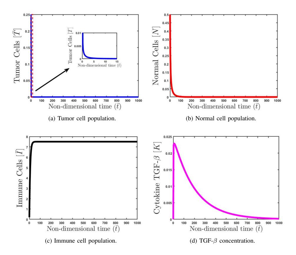
Figure 1: The plot shows the growth behavior of tumor cells, normal cells, immune cells, and the concentration of TGF-\(\beta\). It confirms the stability of the dead equilibrium when \(\psi_1 < \psi_2\) and \(\delta_1 \phi_1 + \phi_2 > \delta_1\). We selected \(\psi_2 = 0.7\), while all other parameters remain constant, as specified in Table 2. The Initial conditions are \(\bar{T} = 0.25, \bar{N} = 0.5, \bar{I} = 0.2\) and \(\bar{K} = 1 \times 10^{-5}\).
3.4. Stability analysis of the coexistence equilibrium
We now find the equilibrium solutions in the presence of tumor cells and TGF-\(\beta\). By equating the equations in model system (4) to zero, the biologically meaningful solutions are:
\[\bar{N}^{**} = \eta_4 - \eta_5 \bar{T}^{**}, \qquad \bar{I}^{**} = \frac{\delta_3 + \bar{T}^{**}}{\eta_2 + \eta_3 \bar{T}^{**}}, \qquad \bar{K}^{**} = \eta_1 \bar{T}^{**},\] (12)
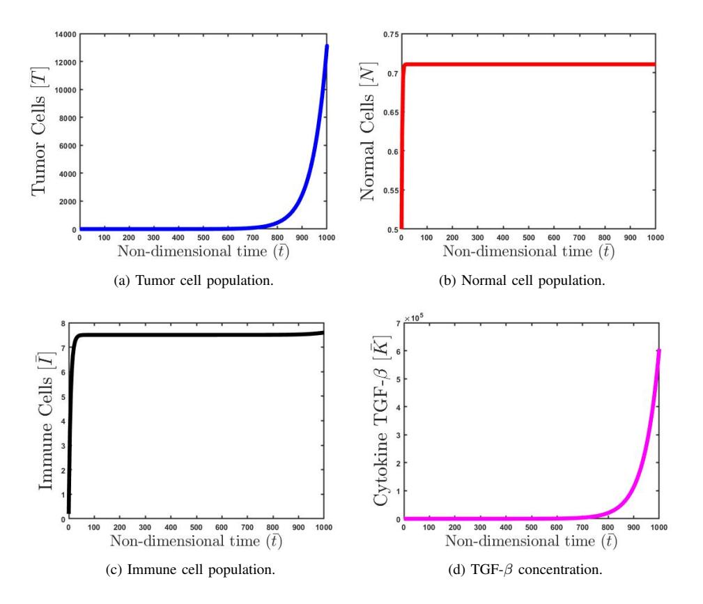
Figure 2: The plot shows the growth behavior of tumor cells, normal cells, immune cells, and the concentration of TGF-β. It confirms the instability of the dead equilibrium when ψ1 > ψ2. All other parameters remain constant, as specified in Table 2. The Initial conditions are T¯ = 0.25, N¯ = 0.5, I¯ = 0.2 and K¯ = 1 × 10⁻⁵ .
where T¯∗∗ satisfy the quadratic equation
\[a_2\bar{T}^2 + a_1\bar{T} + a_0 = 0, (13)\]
with
\[\eta_1 = \frac{1}{\chi}, \qquad \eta_2 = \delta_1 \delta_3, \qquad \eta_3 = \delta_1 - \delta_2, \qquad \eta_4 = \frac{\psi_1 - \psi_2}{\psi_1}, \qquad \eta_5 = \frac{\eta_1 \psi_3}{\psi_1},\] and
\[\begin{split} a_2 &= \eta_1 \eta_3 \eta_5 \phi_3, \\ a_1 &= \phi_2 + \eta_1 \eta_2 \eta_5 \phi_3 + \phi_1 \eta_3 - \eta_1 \eta_3 \eta_4 \phi_3 - \eta_3, \\ a_0 &= \phi_1 \eta_2 + \phi_2 \delta_3 - \eta_2 - \eta_1 \eta_2 \eta_4 \phi_3. \end{split}\]
Note that for positive solutions, the following should satisfy
\[\frac{\psi_2 \chi + \psi_3 \bar{T}^{**}}{\chi \psi_1} < 1 \quad \text{and} \quad \frac{\delta_1 \delta_3 + \delta_1 \bar{T}^{**}}{\delta_2 \bar{T}^{**}} > 1,\] \[a_2 = \eta_1 \eta_3 \eta_5 \phi_3 = \left(\frac{\alpha_K \beta_K}{d_K}\right)^2 \left(\frac{\xi_N N_{Max}}{\alpha_N}\right) \left(\frac{1}{\alpha_T^3}\right) (d_I - p).\] (14)
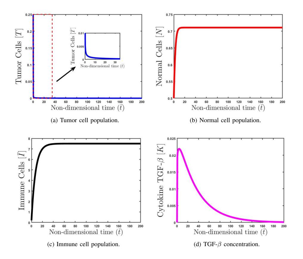
Figure 3: The plot shows the growth behavior of tumor cells, normal cells, immune cells, and the concentration of TGF-\(\beta\). It confirms the stability of the tumor-free equilibrium when \(\delta_1\phi_1+\phi_2+\chi\delta_1>\delta_1\). We have chosen \(\chi=0.05\), and all other parameters remain constant, as specified in Table 2. The Initial conditions are \(\bar{T}=0.25, \bar{N}=0.5, \bar{I}=0.2\) and \(\bar{K}=1\times10^{-5}\).
We can impose that \(p > d_I \implies a_2 < 0\).
\[\begin{split} a_1 &= \phi_2 + \eta_1 \eta_2 \eta_5 \phi_3 + \phi_1 \eta_3 - \eta_1 \eta_3 \eta_4 \phi_3 - \eta_3 \\ &= \left( \frac{\alpha_c s + d_T d_I}{(\alpha_T)^2} + \frac{p d_I \xi_N \alpha_K^2 \beta_K^2}{\alpha_N \alpha_T^4 d_K^2} + \frac{p}{\alpha_T} + \frac{p \alpha_K \beta_K d_N N_{max}}{\alpha_N \alpha_T^2 d_K} \right) - \left( \frac{p d_T}{\alpha_T^2} + \frac{d_I}{\alpha_T} + \frac{d_I \alpha_K \beta_K d_N N_{max}}{d_K \alpha_N \alpha_T^2} \right) \\ &= \frac{\alpha_c s}{\alpha_T^2} + \frac{(d_T - \alpha_T)(d_I - p)}{\alpha_T^2} + \frac{p d_I \xi_N \alpha_K^2 \beta_K^2}{\alpha_N \alpha_T^4 d_K^2} + \frac{\alpha_K \beta_K d_N N_{max}}{d_K \alpha_N \alpha_T^2} (p - d_I). \end{split}\]
Assume that \(\alpha_T > d_T\), and then \(a_1 > 0\), since \(p > d_I\).
\[\begin{split} a_0 &= \phi_1 \eta_2 + \phi_2 \delta_3 - \eta_2 - \eta_1 \eta_2 \eta_4 \phi_3 = \left( \frac{d_I d_T q}{\alpha_T \beta_K} + \frac{q s \alpha_c}{\alpha_T \beta_K} + \frac{q d_I d_N \alpha_K N_{max}}{\alpha_T \alpha_N d_K} \right) - \left( \frac{q d_I}{\beta_k} + \frac{q d_I \alpha_K N_{max}}{\alpha_T d_K} \right) \\ &= \frac{q s \alpha_c}{\alpha_T \beta_K} + \frac{q d_I}{\beta_K} \left( \frac{d_T}{\alpha_T} - 1 \right) + \frac{q d_I \alpha_K N_{max}}{\alpha_T d_K} \left( \frac{d_N}{\alpha_N} - 1 \right). \end{split}\]
We will use Descartes's Rule of signs to discuss the existence of the positive solutions to the equation (13). Table 3 shows all possibilities of positive solutions to equation (13).
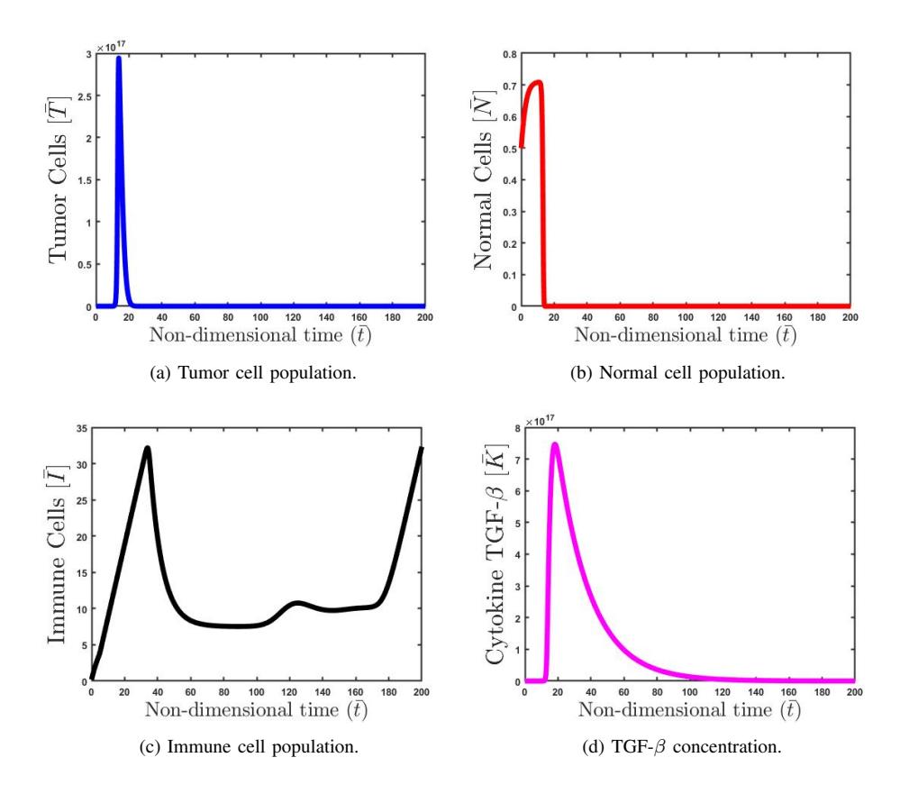
Figure 4: The plot shows the growth behavior of tumor cells, normal cells, immune cells, and the concentration of TGF-\(\beta\). It confirms the instability of the tumor-free equilibrium when \(\delta_1\phi_1+\phi_2+\chi\delta_1<\delta_1\). We have chosen \(\phi_2=0.1,\chi=0.05\), and all other parameters remain constant, as specified in Table 2. The Initial conditions are \(\bar{T}=0.25,\bar{N}=0.5,\bar{I}=0.2\) and \(\bar{K}=1\times 10^{-5}\).
Table 3: Possibilities of positives solutions of Equation (13).
| Case | \(a_2\) | \(a_1\) | \(a_0\) | Number of positive solutions |
|---|---|---|---|---|
| (I) (II) | - | + + | + | 1 2 or 0 |
The solutions of equation (13) are given by
\[\bar{T}^{**} = \frac{-a_1 \pm \sqrt{a_1^2 - 4a_2 a_0}}{2a_2} = \frac{a_1}{2a_2} \left( -1 \pm \sqrt{1 - \frac{4a_0 a_2}{a_1^2}} \right),\tag{15}\]
from Table 3, when \(a_0 > 0\), a unique coexistence equilibrium is obtained as follows:
\[E_1^{**}(\bar{T}_1^{**}, \bar{N}_1^{**}, \bar{I}_1^{**}, \bar{K}_1^{**}) \quad \text{with} \quad \bar{T}^{**} = \frac{a_1}{2a_2} \left( -1 - \sqrt{1 - \frac{4a_0a_2}{a_1^2}} \right),\] (16)
when \(a_0 < 0\), we either have no coexistence equilibrium point when \(\frac{4a_0a_2}{a_1^2} > 1\), or two coexistence equilibrium
points,
\[E_2^{**}(\bar{T}_2^{**}, \bar{N}_2^{**}, \bar{I}_2^{**}, \bar{K}_2^{**})\] and \(E_3^{**}(\bar{T}_3^{**}, \bar{N}_3^{**}, \bar{I}_3^{**}, \bar{K}_3^{**}),\) (17)
as given by equation (15), when \(\frac{4a_0a_2}{a_1^2} < 1\).
Stability analysis of the coexistence equilibrium using Gershgorin circle theorem
To analyze the stability of the coexistence equilibrium point, we will employ the Gershgorin circle theorem [48]. The fundamental idea of this theorem can be outlined as follows:
Let \(J = (J_{ij})_{1 \le i,j \le n}\) be a \(n \times n\) matrix with real coefficients. If the following conditions are satisfied:
1) \[j_{ii} < 0\] for \(1 \le i \le n\).
2) \[R_i < |J_{ii}|\] for \(1 \le i \le n\), where \(R_i = \sum_{j=1, j \ne i}^n |J_{ij}|\)
then, the eigenvalues of J are negative or have negative real parts.
The Jacobean of the model system (4) evaluated at the coexistence equilibrium is
\[J = \begin{pmatrix} 1 - \phi_1 - \phi_2 \bar{I}^{**} & \phi_3 \bar{K}^{**} & -\phi_2 \bar{T}^{**} & \phi_3 \bar{N}^{**} \\ 0 & \psi_1 - 2\psi_1 \bar{N}^{**} - \psi_2 - \psi_3 \bar{K}^{**} & 0 & -\psi_3 \bar{N}^{**} \\ \frac{\delta_2 \delta_3 \bar{I}^{**}}{\left(\delta_3 + \bar{T}^{**}\right)^2} & 0 & -\delta_1 + \frac{\delta_2 \bar{T}^{**}}{\delta_3 + \bar{T}^{**}} & 0 \\ 1 & 0 & 0 & -\gamma \end{pmatrix}, \tag{18}\] where
\[\bar{N}^{**} = \frac{\chi(\psi_1 - \psi_2) - \psi_3 \bar{T_i}^{**}}{\chi \psi_1}, \quad \bar{I}^{**} = \frac{\delta_3 + \bar{T_i}^{**}}{\delta_1 \delta_3 + (\delta_1 - \delta_2) \bar{T_i}^{**}}, \quad \text{and} \quad \bar{K}^{**} = \frac{1}{\chi} \bar{T_i}^{**}, \quad 1 \le i \le 3.\] (19)
By applying conditions (1) and (2) of the Gershgorin circles theorem, the coexistence equilibrium points become locally asymptotically stable if
\[1 - \phi_1 - \phi_2 \bar{I_i}^{**} < 0, \quad \psi_1 - 2\psi_1 \bar{N_i}^{**} - \psi_2 - \psi_3 \bar{K_i}^{**} < 0, \quad \text{and} \quad -\delta_1 + \frac{\delta_2 \bar{T_i}^{**}}{\delta_3 + \bar{T_i}^{**}} < 0, \quad (20)\] or
\[\phi_1 + \phi_2 \bar{I_i}^{**} > 1, \qquad \frac{2\psi_1 \bar{N_i}^{**} + \psi_2 + \psi_3 \bar{K_i}^{**}}{\psi_1} > 1, \qquad \text{and} \qquad \frac{\delta_2 \bar{T_i}^{**}}{\delta_1 (\delta_3 + \bar{T_i}^{**})} < 1, \qquad (21)\]
in the first condition, and the second condition implies
\[\phi_3 \bar{K_i}^{**} + \phi_2 \bar{T_i}^{**} + \left| \phi_3 \bar{N_i}^{**} \right| < \left| 1 - \phi_1 - \phi_2 \bar{I_i}^{**} \right|, \tag{22}\]
\[\psi_3 \bar{N_i}^{**} < \left| \psi_1 - 2\psi_1 \bar{N_i}^{**} - \psi_2 - \psi_3 \bar{K_i}^{**} \right|, \tag{23}\]
\[\frac{\delta_2 \delta_3 \bar{I}_i^{**}}{(\delta_3 + \bar{T}_i^{**})^2} < \left| -\delta_1 + \frac{\delta_2 \bar{T}_i^{**}}{\delta_3 + \bar{T}_i^{**}} \right|, \tag{24}\]
\[\gamma > 1. \tag{25}\]
When we substitute i = 1 into Equations (21), (22), (23), (24), and (25), we obtain the stability conditions for the unique coexistence equilibrium (16). Similarly, substituting i = 2 and i = 3 into Equations (21), (22), (23), (24), and (25), provides us with the stability conditions for the scenario in which we have two coexistence equilibrium points (17).
4. MODEL SIMULATIONS WITHOUT CONTROL VARIABLES
In this section, we present the numerical simulations of model system (1) using MATLAB. The parameter values used in these simulations are given in Table 1. For some of the parameters, we did not find any available data; for that reason, we assumed their values to the point where their numerical simulation became reasonable. The variables in Figure 5 have initial values of \(T(0) = 1 \times 10^3\), \(N(0) = 2 \times 10^4\), \(I(0) = 1 \times 10^2\), and \(K(0) = 1 \times 10^{-3}\). Figure 5 shows the behavior of population interactions over 500 days. The simulations reveal that after 450 days of interaction, tumor cells overcome both normal and immune cells. This numerical solution showed that the host immune system alone is not effective enough to stop the progression of tumor cells. Consequently, the introduction of treatment becomes imperative to impede tumor cell growth. In the next section, we introduce chemotherapy and siRNA treatments in order to eliminate tumors.
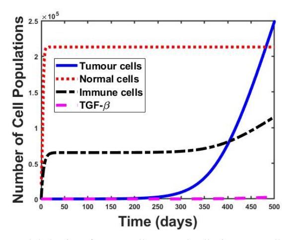
Figure 5: The plot shows the growth behavior of tumor cells, normal cells, immune cells, and the concentration of TGF-\(\beta\) without treatment (without control). It demonstrates that the immune system is not able to eradicate the tumor. The initial conditions are \(T=1\times 10^3\), \(N=2\times 10^4\), \(I=1\times 10^2\), and \(K=1\times 10^{-3}\). The parameter values used in this simulation are listed in Table (1).
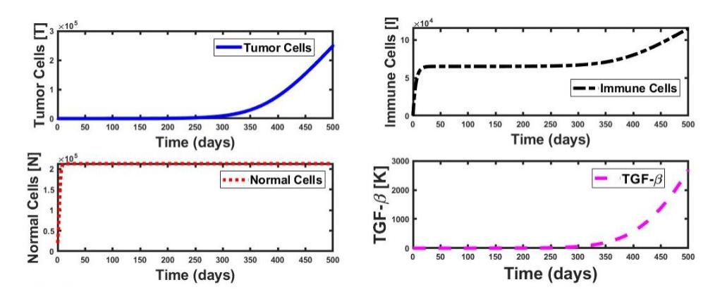
Figure 6: Individual plots depict the behavior of tumor cells (T), normal cells (N), immune cells (I), and the concentration of TGF-\(\beta\) (K) without treatment (control). They illustrate the immune system's inability to eradicate the tumor. The initial conditions are \(T=1\times 10^3\), \(N=2\times 10^4\), \(I=1\times 10^2\), and \(K=1\times 10^{-3}\). The parameter values used in this simulation are listed in Table (1).
5. OPTIMAL CONTROL
In this section, we formulate an optimal control problem for the model system (1) by incorporating the combined effects of chemotherapy and siRNA. The objective is to minimize not only the tumor size and concentration of TGF-\(\beta\), but also the drug-induced toxicity of the treatments to patients. The control variables, \(u_1(t)\) for chemotherapy and \(u_2(t)\) for siRNA, denote the externally administered rates of each drug. These variables are then integrated into the model system (1), resulting in the following control system, which we refer to as the state system
\[\frac{dT}{dt} = (1 - u_1(t))\alpha_T T - d_T T - \alpha_c IT + \beta_K KN - C_T u_1(t)T,\] \[\frac{dN}{dt} = \alpha_N N \left(1 - \frac{N}{N_{Max}}\right) - d_N N - \xi_N KN - C_N u_1(t)N,\] \[\frac{dI}{dt} = s + \frac{pIT}{q+T} - d_I I - C_I u_1(t)I,\] \[\frac{dK}{dt} = (1 - u_2(t))\alpha_K T - d_K K,\] (26)
The term \(1-u_1(t)\) in the first equation represents the drug's primary function blocking tumor cells replication. The last terms \(C_Tu_1(t)T, C_Nu_1(t)N\), and \(C_Iu_1(t)I\), in the first, second, and third equations, respectively, represent toxicity effects of the chemotherapy drug on tumor, normal, and immune cells, with \(C_T, C_N\), and \(C_I\) denoting the toxicity rates. The term \(1-u_2(t)\) in the last equation represents the inhibition of TGF-\(\beta\) production in the presence of siRNA drug. The side effects of siRNA are ignored.
The objective function which is to be minimized is defined as:
\[J(u_1, u_2) = \int_0^{t_f} \left( \mathbf{A}_1 T(t) + \mathbf{A}_2 K(t) + \frac{1}{2} \mathbf{A}_3 u_1^2(t) + \frac{1}{2} \mathbf{A}_4 u_2^2(t) \right) dt \qquad 0 \le t \le t_f, \tag{27}\]
where the coefficients \(A_1\) and \(A_2\) are balancing coefficients associated with the cost of clearing tumor cells and TGF-\(\beta\), while coefficients \(A_3\) and \(A_4\) are associated with the cost of implementing chemotherapy and siRNA, respectively. \(t_f\) represents the termination time of the treatment. The optimal combination of control variables \(u_1\) and \(u_2\) will be adequate to minimize tumor size and TGF-\(\beta\) concentration, as well as negative side effects over a fixed period. The first and second terms of the integrand function represent the tumor size and TGF-\(\beta\) concentration, while the third and fourth terms represent the effectiveness of the applied treatment. In this context, we employ an optimal control problem related to the model to minimize chemotherapy and siRNA administration, aiming to reduce side effects.
We made the assumption that the control variables \(u_1\) and \(u_2\) are bounded and Lebesgue integrable. Consequently, we aim to find an optimal control pair \((u_1^*, u_2^*) \in \Omega\), which minimizes the objective function (27), where
\[\Omega = \{u_1, u_2 : 0 \le u_1(t) \le 1, 0 \le u_2(t) \le 1, 0 \le t \le t_f\},\tag{28}\]
represents the set of admissible controls, with \(u_1(t) = 1\) and \(u_2(t) = 1\) indicating the maximum administration of chemotherapy and siRNA treatments, respectively, and \(u_1(t) = 0\) and \(u_2(t) = 0\) indicating no treatment.
5.1. Necessary conditions for optimality
To find the necessary conditions for our optimal control, we use Pontriagin's Maximum Principle [28]. We begin the optimality by defining the Hamiltonian [29], which is given as follows:
\[H = A_{1}T(t) + A_{2}K(t) + \frac{1}{2}A_{3}u_{1}^{2}(t) + \frac{1}{2}A_{4}u_{2}^{2}(t) + \lambda_{1}\left((1 - u_{1})\alpha_{T}T - d_{T}T - \alpha_{c}IT + \beta_{K}KN - C_{T}u_{1}T\right) + \lambda_{2}\left(\alpha_{N}N\left(1 - \frac{N}{N_{Max}}\right) - d_{N}N - \xi_{N}KN - C_{N}u_{1}N\right) + \lambda_{3}\left(s + \frac{pIT}{q+T} - d_{I}I - C_{I}u_{1}I\right) + \lambda_{4}\left((1 - u_{2})\alpha_{K}T - d_{K}K\right),\] (29)
where λi , 1 ≤ i ≤ 4 are co-state variables satisfying the equations
\[\frac{d\lambda_{1}}{dt} = -\frac{\partial H}{\partial T} = -A_{1} - \lambda_{1} \left( (1 - u_{1})\alpha_{T} - d_{T} - \alpha_{c}I - C_{T}u_{1} \right) - \lambda_{3} \frac{pqI}{(q+T)^{2}} - \lambda_{4}(1 - u_{2})\alpha_{K},\] \[\frac{d\lambda_{2}}{dt} = -\frac{\partial H}{\partial N} = -\lambda_{1}\beta_{K}K - \lambda_{2} \left( \alpha_{N} - \frac{2\alpha_{N}N}{N_{Max}} - d_{N} - \xi_{N}K - C_{N}u_{1} \right),\] \[\frac{d\lambda_{3}}{dt} = -\frac{\partial H}{\partial I} = \lambda_{1}\alpha_{c}T - \lambda_{3} \left( \frac{pT}{q+T} - d_{I} - C_{I}u_{1} \right),\] \[\frac{d\lambda_{4}}{dt} = -\frac{\partial H}{\partial K} = -A_{2} - \lambda_{1}\beta_{K}N + \lambda_{2}\xi_{N}N + \lambda_{4}d_{K},\] (30)
with transversality conditions
\[\lambda_1(t_f) = \lambda_2(t_f) = \lambda_3(t_f) = \lambda_4(t_f) = 0. \tag{31}\]
The optimal controls (u ∗ 1 , u∗ 2 ) ∈ U × U minimizing the Hamiltonian are obtained by solving the equations
\[\frac{\partial H}{\partial u_1} = A_3 u_1 - \lambda_1 \alpha_T T - \lambda_1 C_T T - \lambda_2 C_N N - \lambda_3 C_I I = 0,\] \[\frac{\partial H}{\partial u_1} = A_4 u_2 - \lambda_4 \alpha_K T = 0.\] (32)
Consequently,
\[u_1^* = \frac{\lambda_1 \alpha_T T + \lambda_1 C_T T + \lambda_2 C_N N + \lambda_3 C_I I}{A_3},\tag{34}\]
\[u_2^* = \frac{\lambda_4 \alpha_K T}{A_4}. (35)\]
Imposing the constraints 0 ≤ ui ≤ 1, 1 ≤ i ≤ 2, gives
∂u2
\[u_1^* = \min\left\{\max\left(0, \frac{\lambda_1\alpha_T T + \lambda_1 C_T T + \lambda_2 C_N N + \lambda_3 C_I I}{A_3}\right), 1\right\},\tag{36}\] and u2 ∗ = min max 0, λ4αKT A4 , 1 . (37)
In the next subsection, we will discuss the numerical solutions of our optimal control problem and the treatment strategies we will follow to effectively eradicate cancer.
5.2. Numerical simulations of the model under the effect of chemotherapy and siRNA
In this subsection, we numerically solve our optimal control systems (26) and (30) to observe how the presence of chemotherapy and siRNA treatments can affect the dynamics of tumor cell growth and aid in controlling the tumor. To determine the optimal controls, we employed the forward-backward method to solve the optimality systems (26) and (30). First, we solve the state system (26) forward in time using an initial guess for the optimal controls \((u_1, u_2)\). Then, applying the transversality conditions (31), we solve the costate system (30) backward in time.
As demonstrated in subsection (3.3), tumor-free equilibrium can be obtained via sufficient immune surveillance. In our optimal control model simulations, we choose a scenario where the tumor has escaped immune surveillance and then apply treatments. Chemotherapy is commonly administered for a specific period of time, such as 6 months or a year [45], whereas siRNA can be administered for days or even years [1]. In our simulations, we will extend the treatment period to cover 200 days.
The parameters used in the numerical simulations are the same parameters in Table 1. In all numerical simulations initial conditions for state variables are given by \(T(0) = 9 \times 10^4\), \(N(0) = 1 \times 10^5\), \(I(0) = 5 \times 10^2\) and \(K(0) = 1 \times 10^{-3}\). The weights are given by, \(A_1 = 1 \times 10^5\), \(A_2 = 1 \times 10^2\), \(A_3 = 3 \times 10^3\), \(A_4 = 10\).
We will consider three different treatment scenarios: a) First scenario: chemotherapy only; b) Second scenario: siRNA only; c) Third scenario: Combination of chemotherapy and siRNA. Discussing these three scenarios will allow us to explore the efficacy of each treatment individually and their combined efficacy.
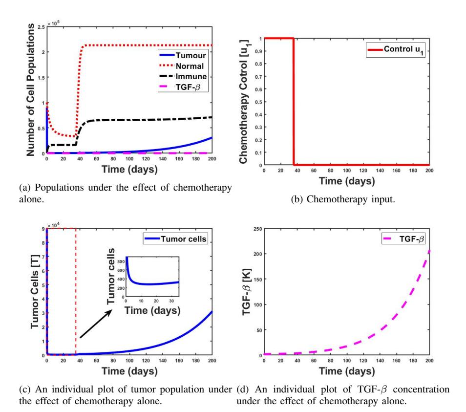
Figure 7: The plot shows the growth behavior of tumor cells (T), normal cells (N), immune cells (I), and the concentration of TGF-\(\beta\) (K) under chemotherapy control. The results show the ability of tumor regrowth and an increase in the concentration of TGF-\(\beta\) during the treatment period. The initial conditions are \(T=9\times10^4\), \(N=1\times10^5\), \(I=5\times10^2\), and \(K=1\times10^{-3}\). The parameter values used in these simulations are listed in Table (1).
a) First scenario: chemotherapy
We examine the scenario where chemotherapy is the only treatment administered to the patient. Throughout our simulation, we maintain \(u_2=0\), for the entire duration, and the results are depicted in Figure 7. During the treatment period, which lasts just under 40 days, as shown in Figure (7b), there is a notable reduction in tumor size as shown in Figure 7c. However, Figure 7c also illustrates that the tumor begins to regrow 20 days after the cessation of treatment. Additionally, an increase in TGF-\(\beta\) levels during this period is observed, alongside the impact of toxicity on normal cells, as depicted in Figure 7a.
b) Second scenario: small interfering RNA (siRNA)
In this scenario, only the molecular therapy of siRNA is administered to the patient. Throughout our simulation, we maintain \(u_1=0\), for the entire duration, and the results are shown in Figure 8. The results demonstrate a rapid decrease in the size of the tumor, which is kept at a low level for most of the treatment period. However, as shown in Figure 8c, there is a possibility of tumor regrowth. Additionally, there is an increase in the levels of TGF-\(\beta\) during this same period, as shown in Figure 8d.
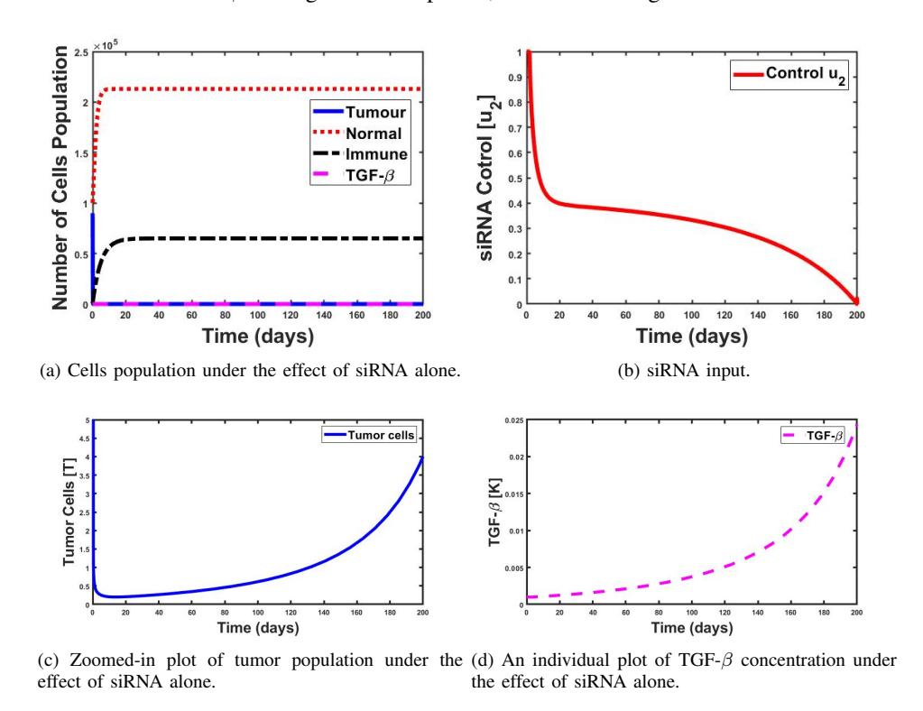
Figure 8: The plot shows the growth behavior of tumor cells (T), normal cells (N), immune cells (I), and the concentration of TGF-\(\beta\) (K) under siRNA control. The results show the ability of tumor regrowth and an increase in the concentration of TGF-\(\beta\) during the treatment period. The initial conditions are \(T=9\times10^4\), \(N=1\times10^5\), \(I=5\times10^2\), and \(K=1\times10^{-3}\). The parameter values used in these simulations are listed in Table (1).
c) Third scenario: chemotherapy and siRNA
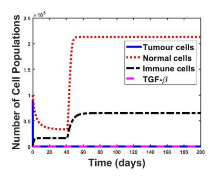
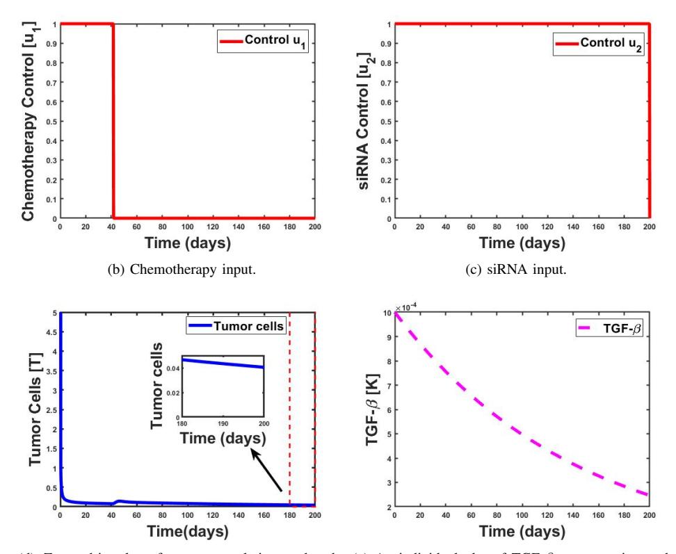
In our final scenario, we aim to prevent tumor regrowth and the increase in the concentration of TGF-\(\beta\) by combining both chemotherapy and siRNA. The results are shown in Figure 9, demonstrate a rapid decrease in tumor size to very low levels during the treatment period, as presented in Figure 9d. Furthermore, it is worth noting the decrease in TGF-\(\beta\) levels during this time, as shown in Figure 9e.
(a) Cell populations under the effect of chemotherapy and siRNA.
(d) Zoomed-in plot of tumor population under the (e) An individual plot of TGF-\(\beta\) concentration under effect of chemotherapy and siRNA.
Figure 9: The plot shows the growth behavior of tumor cells (T), normal cells (N), immune cells (I), and the concentration of TGF-\(\beta\) (K) under the combined control of chemotherapy and siRNA. The results show a decrease in tumor size and in the concentration of TGF-\(\beta\) during the treatment period. The initial conditions are \(T = 9 \times 10^4\), \(N = 1 \times 10^5\), \(I = 5 \times 10^2\), and \(K = 1 \times 10^{-3}\). The parameter values used in these simulations are listed in Table (1).
By comparing the cases of chemotherapy, siRNA treatment, and their combination, we conclude that the combined approach is the most effective in reducing tumor size. However, it should be noted that while this combined approach showed better results, it did not completely eliminate tumor cells but rather reduced them to very low levels.
Figure 9 demonstrates that tumor size and TGF-β concentration can be significantly reduced by administering a combination of chemotherapy and siRNA for 200 days. Our optimal control strategy suggests ceasing chemotherapy after 40 days and continuing siRNA until the end of the treatment period. This approach is meaningful for several reasons. Firstly, ceasing chemotherapy after 40 days, once the tumor cells have been reduced to a very low level, helps minimize the side effects that chemotherapy could cause to normal and immune cells. Additionally, continuing siRNA treatment for 200 days is crucial to prevent cancer recurrence by reducing the concentration of TGF-β to a very low level. Furthermore, an increase in TGF-β can contribute to cancer recurrence, making prolonged siRNA treatment necessary.
Moreover, these results align with clinical evidence. Barnard et al. [54] demonstrated that chemotherapy can extend for 40 days or more. For siRNA treatment implementations, we found variations in clinical trial durations [1], [57], [58]. The protocol in this paper approximates the best treatment strategy, pending further clinical trials.
6. CONCLUSION
In this paper, we investigated the dynamic interactions among tumor cells, normal cells, immune cells, and TGF-β. These interactions are modeled using a system of non-linear differential equations. The stability analysis of the system was conducted, examining dead, tumor-free, and coexistence equilibrium states through eigenvalues and Gershgorin circle theorem criteria. Numerical simulations were performed to observe the system's behavior in the absence of treatment. These simulations showed that tumor cells could overcome normal and immune cells after 450 days of interactions.
We examined the model under the effects of chemotherapy and siRNA treatments. Optimal control theory using Pontryagin's maximum principle is applied to determine the optimal drug dosing strategy. This strategy aimed at minimizing tumor size, the concentration of transforming growth factor-beta, and reducing chemotherapy and siRNA-induced toxicity in patients. Three scenarios were examined to assess the efficacy of these treatments individually and in combination.
The first scenario focused on chemotherapy as the primary approach for tumor therapy, but it demonstrated limited effectiveness in eradicating tumor cells. Where a full dosage of chemotherapy is given for nearly 40 days, and after 20 days of stopping the treatment, tumor cells regrew, accompanied by an increase in the concentration of TGF-β during the treatment period. In the second scenario, we focused on siRNA treatment. By reducing the dosage of siRNA and extending the treatment period to nearly 200 days, tumor cell levels were reduced to a very low level. However, despite this initial success, tumor regrowth occurred subsequently. Additionally, an increase in the concentration of TGF-β is observed, which has the potential to stimulate tumor regrowth. The third and final scenario explored a combination therapy involving both chemotherapy and siRNA, which showed promising outcomes in reducing the population of tumor cells and the concentration of TGF-β. Despite not achieving complete eradication, this approach involved administering full dosages of chemotherapy and siRNA for approximately 40 and 200 days, respectively. Overall, it resulted in significant decreases in tumor size and TGF-β concentration.
The findings presented here align with those reported in [1], [49], [50]. Teicher et al. [49] reported that tumors secreting high levels of TGF-β are more resistant to chemotherapy. Figure (7d) substantiates this finding, illustrating the increase in siRNA concentration, which, in turn, promotes tumor regrowth, as depicted in Figure (7c). Arciero et al. [1] demonstrated that siRNA alone is not capable of eradicating tumor cells from the body; instead, it reduces their size. Figure (8c) shows tumor regrowth after reduction to low levels, providing robust evidence for this observation. Furthermore, Chen et al. [50] indicated that targeting the pathways of TGF-β by siRNA enhances chemotherapy efficacy. Figures (9d) and (9e) serve as compelling evidence, showing a substantial decrease in both tumor cells and TGF-β to extremely low levels.
ACKNOWLEDGEMENT
We are thankful for the financial support from the University of KwaZulu-Natal.