

1. Introduction
The COVID-19 pandemic, which originated in Wuhan, China, has taken a significant toll on the world's population and global economy. The world's first COVID-19 patient was reported in late January 2020, who was a Chinese national [1]. In the middle of 2023, over 600,000,000 people were infected with COVID-19 and over 5,000,000 people died. Further, over 500,000,00 people have been recovered [2]. Concerning the disease, it is consisted of basic symptoms like cough, fever, and sore throat and the mortality rates are relatively high due to pneumonia and alveolar damage caused by the virus. Thus, on March 08, 2020, the World Health Organization (WHO) declared COVID-19 as a pandemic [3]. Nevertheless, it is possible for viruses that spread among humans to change from their original strains over time. When these changes are significantly different from the original virus, they are called "variants". As the SARS-CoV-2 virus, the virus that causes COVID-19 was spreading globally, its variants were identified in many countries around the world and due to the extreme spread of COVID-19, every country paid close attention to controlling its spread [4]. Moreover, Sri Lanka started reporting cases of COVID-19 from 10th of March 2020. Since the main reason for the spread of any virus is the mobility of people, the main measures taken by almost every country, including Sri Lanka, to control COVID-19 can be mentioned as limiting public gatherings, banning travel to
*Corresponding author
Received June \(23^{rd}\), 2023, Revised September \(8^{th}\), 2023 (first), Revised March \(4^{th}\), 2024 (second), Accepted for publication April \(15^{th}\), 2024. Copyright ©2024 Published by Indonesian Biomathematical Society, e-ISSN: 2549-2896, DOI:10.5614/cbms.2024.7.1.2
selected countries, and closing airports to control the arrival of tourists from other countries, closing schools all over the island and finally imposing lockdown laws in rural or urban or the whole country, etc [5]. In such a situation, each and every government expected to deficit the spread of COVID-19 by minimizing the interaction between infected and susceptible populations.
Many countries were not successful in clearly identifying the periods that they should implement and remove lockdown to minimize the harm that it causes to the economy. As a result, several nations had to experience severe economic calamities. Especially the importation of vaccines for the control of COVID-19 and the collapse of the tourism industry, which is a major source of foreign exchange inflows to Sri Lanka, undoubtedly indicates a drain on Sri Lanka's dollar reserves. Hence, various epidemic models related to COVID-19 and the Optimal Control Theory were developed and this particular study is also a result of that.
Concerning the global context, the SEIVR model has been developed using three control variables for isolation, vaccine efficacy and treatment enhancement [6]. An extended SEIR model has been proposed to control the spread of COVID-19 utilizing Kalman filter (ENKF) models as a data assimilation method [3]. Further, deterministic compartmental epidemiological model was also designed to study the third wave of the epidemic in the country using the Optimal control measures to reduce the burden of the disease. Nevertheless, it is noted that they have not considered demographic features in that study [7]. The optimal control of the COVID-19 pandemic can be considered with Non-Pharmaceutical Interventions. Thus, a study has been conducted using the optimal control analysis of a mathematical model of SARS-CoV-2 transmission from May 2020 to December 2021 [8]. Furthermore, a two-stage epidemic model with a dynamic control strategy was further developed to define the spread of the 2019 Coronavirus. In that study, appropriate controlling mechanisms were brought out to minimize the controlling cost of the disease and to ensure the effective functioning of society [9].
The SIR model has been formulated in this research using optimal control theory to identify how human mobility can be controlled to reduce the spread of COVID-19. Thus, three collective main regions in Sri Lanka were considered. The values for the normal mobility rate between and within the regions were calculated using the population data of Sri Lanka and the gravity model. In each region, COVID-19 data of infected, susceptible and recovery populations in 2021 was retrieved from March to April [10]. Further, the disease transmission rate and recovery rate were calculated using the COVID-19 data and the least square estimation. In developing this SIR model, two control variables were used to control human mobility within and between the region. Therefore, by examining the behavior of the control variables, it was possible to get a clear idea regarding the timelines to maintain the lockdown conditions between and within the regions to deficit the spread of COVID-19. Thus, the main purpose of this model is to present an idea regarding the systematic imposition and removal of lockdown laws in the event of a disaster like COVID-19 in the future.
2. MODEL FORMULATION
2.1. Model and optimal control strategy
The optimal control theory has been used in this research for a susceptible-infected-recovered (SIR) model which is designed based on the mobility of the population for the spread of COVID-19 in Sri Lanka. Thus, it is assumed that human population dynamics (birth and death rates) are insignificant and the human population in each region is constant. Furthermore, optimal control strategies are used to minimize the number of infected populations. The Pontryagin's maximum principle has been mainly used here. For this research, 25 districts in Sri Lanka are divided into three regions. A Region 01 has been created concerning the districts of Colombo, Gampaha, and Kalutara, which are the centre of the spread of COVID-19 in Sri Lanka, and all the other districts around those districts are divided into two more regions. Hence, Region 02 encompasses Puttalam, Kurunegala, Ratnapura, Galle, Matara and kegalla; and Region 03 contains all other districts. Populations percentage of Region 01, Region 02 and Region 03 are depicted by figure 2.1 below and their population density(people per square kilometer) are respectively 1588.3, 391.8 and 180.4.
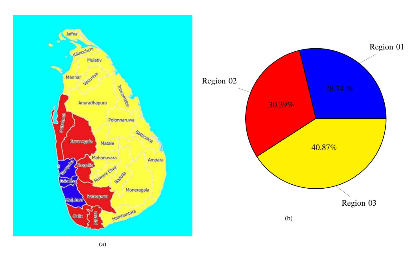
Figure 1: (a). Region 01: Blue Color, Region 02: Red Color , Region 03: yellow Color, (b). Percentage of population
Definitions of variables and parameters used for model formulation in this research are shown in Table 1.
Table 1: Description of parameters.
| Variable/Parameter | Description |
|---|---|
| i | Region number (i = 1, 2, 3) |
| Si(t) | Number of susceptible individuals at region i at time t |
| Ii(t) | Number of infected individuals at region i at time t |
| Ri(t) | Number of recovered individuals at region i at time t |
| N | Total Population (N = Si + Ii + Ri) |
| mij | Rate of mobility from region i and j at time t |
| uij | Rate of mobility from region i and j at time t considering the lockdown effect |
| β | Infection rate |
| γ | Recovery rate |
| wi | Weight constants |
2.2. Mobility
To determine the mobility rate (m11) for the Region 01, the ratio has been computed between the sum of the population density of the districts in the Region 01 and the sum of the population density of all the districts of Sri Lanka. The m11 is around 0.48. The methodology used to compute the mobility rate in the
Region 01 is also used to calculate it in the other two. The mobility rates for the Region 02 and Region 03 are 0.22 (m22) and 0.29 (m33), respectively. The mobility rate between regions was calculated based on the results obtained from the gravity model (P1P2/r2 ) [12]. Nevertheless, in this occasion, the population of the two regions under consideration is used in place of P1 and P2, and r is considered as the average distance between the two regions. To determine the mobility rate between Region 01 and Region 02 (m12), the value obtained from the gravity model between these two regions was divided by the total sum of the values obtained from the gravity model between each of the two regions. The same method was also used to calculate the mobility rates between Region 01 and Region 03, Region 02 and Region 03. Those values are presented in the table below.
Table 2: Mobility rates (between regions).
| Between Regions (i and j) | Mobility Rates (mij ) | Mobility Rate Values |
|---|---|---|
| 1 and 2 | m12 | 0.64 |
| 1 and 3 | m13 | 0.16 |
| 2 and 3 | m23 | 0.19 |
In this research, optimal mobility control variables (u1, u2) were used as a weight term with normal human mobility rates to optimize the effect of normal human mobility rates within and between regions on the spread of disease. The values of these optimal mobility control variables are maintained in the value range between 0 and 1. Thus, depending on the value of these optimal mobility control variables, the human mobility condition within and between the regions can be described as follows.
1. Full lockdown scenario:
u1 = 0 and u2 = 0 are shown to be under full lockdown within and between regions, respectively. The minimum values of u1 and u2 are not maintained to be 0 based on the continuous provision of services like food and medicine to the people and maintaining a certain level of economic activity.
2. Fully open scenario:
When both u1 and u2 are set to 1, travel restrictions are lifted within and between regions.
However, the effect of the disease may occur from time to time until the disease is completely eradicated, so within each region and between each region, a fully open state is not maintained. For this, things such as bringing only essential staff to service stations, using reduced capacity in public transport, etc., can be implemented. Here, the initial and final values of u1 and u2 can be determined according to the disease spread status of each region and according to the opinions of economists, epidemiologists and public health experts. For example, suppose u1 = 0.5 and u2 = 0.4. This means that human mobility within and between the regions is at a moderate level. Then, public transport services can transport passengers and employees to offices, etc., to a certain level. Furthermore, the essential services prescribed by the government can be maintained between the regions as per the advice of experts.
In addition, the mathematical model which was derived by incorporating the mobility and the control to the SIR model can be represented by a system of non-linear ordinary differential equations as follows:
\[\dot{S}_{i} = -\beta u_{1} m_{ii} S_{i} I_{i} - \beta \sum_{\substack{j=1\\i \neq j}}^{3} u_{2} m_{ij} S_{i} I_{j}, \dot{I}_{i} = \beta u_{1} m_{ii} S_{i} I_{i} + \beta \sum_{\substack{j=1\\i \neq j}}^{3} u_{2} m_{ij} S_{i} I_{j} - \gamma I_{i}, \dot{R}_{i} = \gamma I_{i}, \dot{i} = 1, 2, 3.\] (1)
Control system (1) involves three state variables: susceptible human proportion in patch i,Si(t), infected human proportion in patch i, Ii(t), recovered human proportion in patch i, Ri(t) (t ≥ 0). The infection and recovery rates are taken as \(\beta=0.2\) and \(\gamma=0.01\) respectively. These rates were computed using COVID-19 data from 2021 from April 15 to May 15 [10]. Here, the SIR model was implemented least square minimization on the difference of data and model simulation. In this case common mobility rate (m) for all \(m_{ij}\)'s were used instead of those included in the SIR model presented in (1) above. In selecting a value for the common mobility rate, Region 01 and Region 02 (0.64) have been considered, which have been more affected by the spread of COVID-19 in Sri Lanka. For this, the SIR system with a common mobility rate was used as follows:
\[\dot{S} = -m\beta SI,\] \[\dot{I} = m\beta SI - \gamma I,\] \[\dot{R} = \gamma I.\] (2)
2.3. Cost functional and solving tools
The optimal control problem aims to minimize the proportions of infected humans in three regions over a finite time horizon at the lowest possible implementation cost is given as follows:
\[J(I_1, I_2, I_3, u_1, u_2) = \min \int_0^{t_f} \left[ \sum_{i=1}^3 w_i I_i(t) + w_{(j+3)} \sum_{j=1}^2 (1 - u_j(t))^2 \right] dt,\] (3)
where \(w_1, w_2, w_3, w_4\) and \(w_5\) are weight constants on the infected human in Region 01, Region 02, and Region 03 respectively and the control variables. Then, we need to identify an optimal pair \((U^*, X^*)\) such that,
\[J(U^*) = min\{J(U)|U \in \Omega\}\] where \(\Omega=\{u_i(t)\in (L^1(0,t_f))^2\}\|\) \(a_i\leq u_i(t)\leq b_i\), \(t\in (0,t_f)\), i=1,2 subject to state equations (1) with \(X=(S_1,I_1,R_1,S_2,I_2,R_2,S_3,I_3,R_3)\) and \(U=(u_1,u_2)\). Further, \(a_i\) and \(b_i\) are lower and upper bound of the control \((u_i)\). The standard results of optimal control theory provide a guarantee for the existence of optimal controls [13]. The Pontryagin's maximum principle is used to find the necessary conditions for optimal solutions [14]. This principle is used to convert the system (1) into the problem of minimizing the Hamiltonian H given by:
\[H = w_{1}I_{1}(t) + w_{2}I_{2}(t) + w_{3}I_{3}(t) + w_{4}(1 - u_{1}(t))^{2} + w_{5}(1 - u_{2}(t))^{2}\] \[- \lambda_{1}\beta S_{1}(u_{1}m_{11}I_{1} + u_{2}m_{12}I_{2} + u_{2}m_{13}I_{3})\] \[+ \lambda_{2}\beta S_{1}(u_{1}m_{11}I_{1} + u_{2}m_{12}I_{2} + u_{2}m_{13}I_{3}) - (\lambda_{2}\gamma I_{1})\] \[+ \lambda_{3}\gamma I_{1}\] \[- \lambda_{4}\beta S_{2}(u_{1}m_{22}I_{2} + u_{2}m_{12}I_{1} + u_{2}m_{23}I_{3})\] \[+ \lambda_{5}\beta S_{2}(u_{1}m_{22}I_{2} + u_{2}m_{12}I_{1} + u_{2}m_{23}I_{3}) - (\lambda_{5}\gamma I_{2})\] \[+ \lambda_{6}\gamma I_{2}\] \[- \lambda_{7}\beta S_{3}(u_{1}m_{33}I_{3} + u_{2}m_{13}I_{1} + u_{2}m_{23}I_{2})\] \[+ \lambda_{8}\beta S_{3}(u_{1}m_{33}I_{3} + u_{2}m_{13}I_{1} + u_{2}m_{23}I_{2}) - (\lambda_{8}\gamma I_{3})\] \[+ \lambda_{9}\gamma I_{3}\] \[(4)\]
Theorem 2.1. There exist optimal controls \(U^*(t)\) and corresponding state solutions \(X^*(t)\) that minimize J(U) over \(\Omega\) In order for the above statement to be true, it is necessary that there exist continuous functions \(\lambda_i(t)\) such that [15],
\[\frac{\partial \lambda_{1}}{\partial t} = -\frac{\partial H}{\partial S_{1}} = (\lambda_{1} - \lambda_{2})\beta(u_{1}m_{11}I_{1} + u_{2}m_{12}I_{2} + u_{2}m_{13}I_{3}),\] \[\frac{\partial \lambda_{2}}{\partial t} = -\frac{\partial H}{\partial I_{1}} = -w_{1} + (\lambda_{1} - \lambda_{2})\beta u_{1}m_{11}S_{1} + (\lambda_{4} - \lambda_{5})\beta u_{2}m_{12}S_{2} + (\lambda_{7} - \lambda_{8})\beta u_{2}m_{13}S_{3} - \lambda_{3}\gamma + \lambda_{2}\gamma,\] \[\frac{\partial \lambda_{3}}{\partial t} = -\frac{\partial H}{\partial R_{1}} = 0,\] \[\frac{\partial \lambda_{4}}{\partial t} = -\frac{\partial H}{\partial S_{2}} = (\lambda_{4} - \lambda_{5})\beta(u_{1}m_{22}I_{2} + u_{2}m_{12}I_{1} + u_{2}m_{23}I_{3}),\] \[\frac{\partial \lambda_{5}}{\partial t} = -\frac{\partial H}{\partial I_{2}} = -w_{2} + (\lambda_{1} - \lambda_{2})\beta u_{2}m_{12}S_{1} + (\lambda_{4} - \lambda_{5})\beta u_{1}m_{22}S_{2} + (\lambda_{7} - \lambda_{8})\beta u_{2}m_{23}S_{3} - \lambda_{6}\gamma + \lambda_{5}\gamma,\] \[\frac{\partial \lambda_{6}}{\partial t} = -\frac{\partial H}{\partial R_{2}} = 0,\] \[\frac{\partial \lambda_{7}}{\partial t} = -\frac{\partial H}{\partial S_{3}} = (\lambda_{7} - \lambda_{8})\beta(u_{1}m_{33}I_{3} + u_{2}m_{13}I_{1} + u_{2}m_{23}I_{2}),\] \[\frac{\partial \lambda_{8}}{\partial t} = -\frac{\partial H}{\partial I_{3}} = -w_{3} + (\lambda_{1} - \lambda_{2})\beta u_{2}m_{13}S_{1} + (\lambda_{4} - \lambda_{5})\beta u_{2}m_{23}S_{2} + (\lambda_{7} - \lambda_{8})\beta u_{1}m_{33}S_{3} - \lambda_{9}\gamma + \lambda_{8}\gamma,\] \[\frac{\partial \lambda_{9}}{\partial t} = -\frac{\partial H}{\partial R_{3}} = 0.\] (5)
Now we can obtain optimality conditions by using transversality conditions λi(tf ) = 0 for i = 1, 2, 3, ..., 9 [14].
\[u_{1}^{*} = min \left\{ b_{1}, max \left\{ a_{1}, \frac{2w_{4} + (\lambda_{1} - \lambda_{2})\beta m_{11}S_{1}I_{1} + (\lambda_{4} - \lambda_{5})\beta m_{22}S_{2}I_{2} + (\lambda_{7} - \lambda_{8})\beta m_{33}S_{3}I_{3}}{2w_{4}} \right\} \right\},\] \[u_{2}^{*} = min \left\{ b_{2}, max \left\{ a_{2}, \frac{1}{2w_{5}} \left[ 2w_{5} + (\lambda_{1} - \lambda_{2})\beta (m_{12}S_{1}I_{2} + m_{13}S_{1}I_{3}) + (\lambda_{4} - \lambda_{5})\beta (m_{12}S_{2}I_{1} + m_{23}S_{2}I_{3}) + (\lambda_{7} - \lambda_{8})\beta (m_{13}S_{3}I_{1} + m_{23}S_{3}I_{2}) \right] \right\} \right\}.\] \[(6)\]
As the attainment of analytical solutions for the above model is complicated, a forward-backward sweep has been used to get numerical solutions [14]. A Matlab code is designed and considered getting initial, susceptible, infected, and recovered in each region. Initially, the COVID-19 data report for Sri Lanka from 2021 from April 15 to May 15 were analyzed, and the infected population of the three major regions which has been mentioned previously was recorded [10]. Through the development of the SIR model, it has investigated how human mobility across three regions affected the COVID-19 outbreak. Moreover, it is vital to note that the rates of mobility between the i and j regions as well as j and i in the research have been assumed to be identical. Additionally, it is assumed that everyone who traveled from region i to region j at the beginning of the day will return to region i at the end of the day.
2.4. Effective reproductive number (Rt)
The effective reproductive number can be calculated by the product of the basic reproductive number and the proportion of the host population that is susceptible (S(t)) [11],
\[R_t = R_0 S(t). (7)\]
The basic reproductive number (R0) is calculated by using the the next generation matrix approach. Let x = (I1, I2, I3) T ; f(x) represents all the new infections. The net transition rates out of the corresponding
compartment are represented by v(x) [15]:
\[f(x) = \begin{pmatrix} \beta S_1(u_1 m_{11} I_1 + u_2 m_{12} I_2 + u_2 m_{13} I_3) \\ \beta S_2(u_1 m_{22} I_2 + u_2 m_{12} I_1 + u_2 m_{23} I_3) \\ \beta S_3(u_1 m_{33} I_3 + u_2 m_{13} I_1 + u_2 m_{23} I_2) \end{pmatrix} and \quad v(x) = \begin{pmatrix} \gamma I_1 \\ \gamma I_2 \\ \gamma I_3 \end{pmatrix},\](8)
where the matrices \(\frac{\partial f}{\partial x_i}(x^*)\) and \(\frac{\partial v}{\partial x_i}(x^*)\) at the disease-free equilibrium, \(x^*(i=1,2,3)\) can be defined as follows[16]:
.
\[F = \begin{pmatrix} \frac{\partial f_1}{\partial I_1} & \frac{\partial f_1}{\partial I_2} & \frac{\partial f_1}{\partial I_3} \\ \frac{\partial f_2}{\partial I_1} & \frac{\partial f_2}{\partial I_2} & \frac{\partial f_2}{\partial I_3} \\ \frac{\partial f_3}{\partial I_1} & \frac{\partial f_3}{\partial I_2} & \frac{\partial f_3}{\partial I_3} \end{pmatrix} = \begin{pmatrix} \beta u_1 m_{11} & \beta u_2 m_{12} & \beta u_2 m_{13} \\ \beta u_2 m_{12} & \beta u_1 m_{22} & \beta u_2 m_{23} \\ \beta u_2 m_{13} & \beta u_2 m_{23} & \beta u_1 m_{33} \end{pmatrix},\](9)
\[V = \begin{pmatrix} \frac{\partial v_1}{\partial I_1} & \frac{\partial v_1}{\partial I_2} & \frac{\partial v_1}{\partial I_3} \\ \frac{\partial v_2}{\partial I_1} & \frac{\partial v_2}{\partial I_2} & \frac{\partial v_2}{\partial I_3} \\ \frac{\partial v_3}{\partial I_1} & \frac{\partial v_3}{\partial I_2} & \frac{\partial v_3}{\partial I_3} \end{pmatrix} = \begin{pmatrix} r & 0 & 0 \\ 0 & r & 0 \\ 0 & 0 & r \end{pmatrix}.\] (10)
Next, the matrix \(A=FV^{-1}\) can be defined as follows:
\[V^{-1} = \begin{pmatrix} \frac{1}{r} & 0 & 0\\ 0 & \frac{1}{r} & 0\\ 0 & 0 & \frac{1}{r} \end{pmatrix},\tag{11}\]
\[A = FV^{-1} = \begin{pmatrix} \frac{\beta u_1 m_{11}}{r} & \frac{\beta u_2 m_{12}}{r} & \frac{\beta u_2 m_{13}}{r} \\ \frac{\beta u_2 m_{12}}{r} & \frac{\beta u_1 m_{22}}{r} & \frac{\beta u_2 m_{23}}{r} \\ \frac{\beta u_2 m_{13}}{r} & \frac{\beta u_2 m_{23}}{r} & \frac{\beta u_1 m_{33}}{r} \end{pmatrix}.\](12)
The eigenvalues of matrix A can be calculated by using \(|A - \lambda I| = 0\) as follows:
\[|A - \lambda I| = \left| \begin{pmatrix} \frac{\beta u_1 m_{11}}{r} & \frac{\beta u_2 m_{12}}{r} & \frac{\beta u_2 m_{13}}{r} \\ \frac{\beta u_2 m_{12}}{r} & \frac{\beta u_1 m_{22}}{r} & \frac{\beta u_2 m_{23}}{r} \\ \frac{\beta u_2 m_{13}}{r} & \frac{\beta u_2 m_{23}}{r} & \frac{\beta u_1 m_{33}}{r} \end{pmatrix} - \lambda \begin{pmatrix} 1 & 0 & 0 \\ 0 & 1 & 0 \\ 0 & 0 & 1 \end{pmatrix} \right| = 0, \tag{13}\]
\[|A - \lambda I| = \left| \begin{pmatrix} \left(\frac{\beta u_1 m_{11}}{f} - \lambda\right) & \frac{\beta u_2 m_{12}}{r} & \frac{\beta u_2 m_{13}}{r} \\ \frac{\beta u_2 m_{12}}{r} & \left(\frac{\beta u_1 m_{22}}{f} - \lambda\right) & \frac{\beta u_2 m_{23}}{r} \\ \frac{\beta u_2 m_{13}}{r} & \frac{\beta u_2 m_{23}}{r} & \left(\frac{\beta u_1 m_{33}}{r} - \lambda\right) \end{pmatrix} \right| = 0.\] (14)
Thus, the basic reproductive number (dominant eigenvalue of \(FV^{-1}\)) for the three patch system can be calculated by solving the following cubic equation.
\[\lambda^{3} - \left(\frac{\beta u_{1} m_{11}}{r} + \frac{\beta u_{1} m_{22}}{r} + \frac{\beta u_{1} m_{33}}{r}\right) \lambda^{2} + \left(\frac{\beta^{2} u_{1}^{2} m_{11} m_{22}}{r^{2}} + \frac{\beta^{2} u_{1}^{2} m_{11} m_{33}}{r^{2}} - \frac{\beta^{2} u_{2}^{2} m_{12}^{2}}{r^{2}} - \frac{\beta^{2} u_{2}^{2} m_{13}^{2}}{r^{2}} + \frac{\beta^{2} u_{1}^{2} m_{22} m_{33}}{r^{2}} - \frac{\beta^{2} u_{2}^{2} m_{23}^{2}}{r^{2}}\right) \lambda - \frac{\beta^{3} u_{1}^{3} m_{11} m_{22} m_{33}}{r^{3}} + \frac{\beta^{3} u_{1} u_{2}^{2} m_{11} m_{23}^{2}}{r^{3}} + \frac{\beta^{3} u_{1} u_{2}^{2} m_{12} m_{33}}{r^{3}} - \frac{2\beta^{3} u_{2}^{3} m_{12} m_{23} m_{13}}{r^{3}} + \frac{\beta^{3} u_{1} u_{2}^{2} m_{13}^{2} m_{22}}{r^{3}} = 0.\] (15)
Symbolic expressions for three eigenvalues can be obtained by solving the above cubic equation. By substituting the values for the mobility control variable, mobility rate, infection rate, and recovery rates contained therein, values for three real eigenvalues can be obtained. Then the dominant eigenvalue can be taken as the basic reproductive number. An important point here is that the expressions obtained for the eigenvalues contain control variables that change with time, so it can be indicated that an exact symbolic expression for the dominant eigenvalue cannot be presented. Because the resulting eigenvalue is obtained at a time point, the variation of the basic reproductive number with time is represented graphically in Figure 5.
3. RESULTS
A description of the results of the SIR model designed by the researchers is carried out in two main sections; the first with and without the mobility controls (u1 and u2) and observing how the infected population in three regions changes over time. After that, a sensitivity analysis is done by changing the weight constants (w1, w2, w3) and the upper and lower bounds of u1 and u2 with time to observe the variations in u1 and u2. Further, the weight constants w4 and w5 are set as 0.4 for realistic simulations.
The variation of the infected human proportion with time is shown in Figure 2.
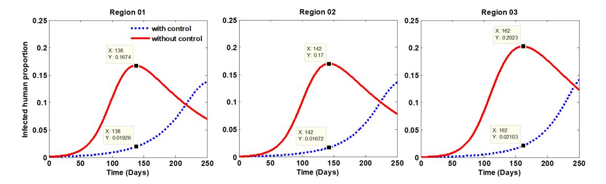
Figure 2: Behavior of the infected human proportion (x= time , y=infected human proportion) (w1 = 1; w2 = 1; w3 = 1; γ = 0.01; β = 0.2; m11 = 0.48; m22 = 0.22; m33 = 0.29; m12 = 0.64; m13 = 0.16; m23 = 0.19; 0.2 ⩽ u1 ⩽ 0.9; 0.1 ⩽ u2 ⩽ 0.8).
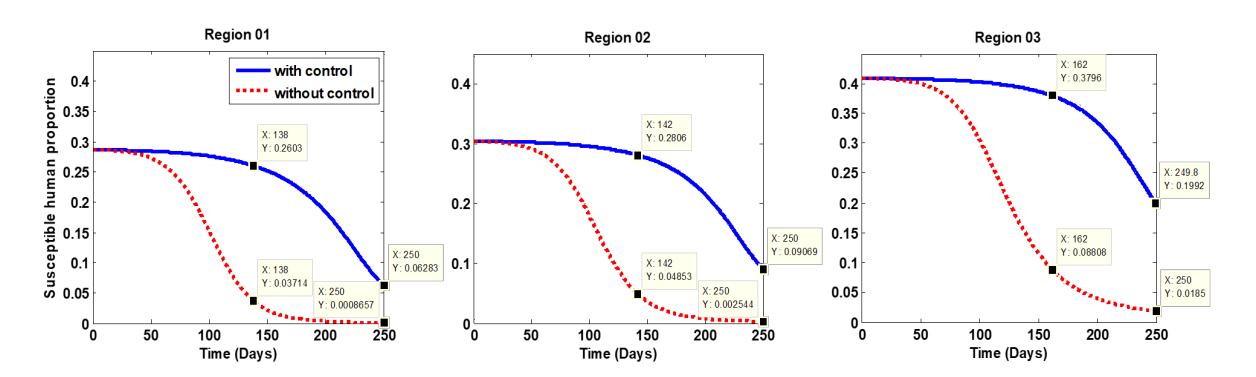
Figure 3: Behavior of the susceptible human proportion (x= time , y= susceptible human proportion) (w1 = 1; w2 = 1; w3 = 1; γ = 0.01; β = 0.2; m11 = 0.48; m22 = 0.22; m33 = 0.29; m12 = 0.64; m13 = 0.16; m23 = 0.19; 0.2 ⩽ u1 ⩽ 0.9 ; 0.1 ⩽ u2 ⩽ 0.8).
After analyzing the infected human proportions over time, it was observed that the infected human proportion has reached peak levels of 0.1674, 0.17, and 0.2023 in the Region 01, Region 02, and Region 03, respectively, at 138 days, 142 days, and 162 days when mobility controls (u1 and u2) were deactivated. The variation of the susceptible human proportion with time is given in Figure 3. After analyzing the susceptible human proportions over time, it was evident that at the end of 250 days, the values of susceptible human proportions in all three regions were higher when mobility controls were activated, compared to when the controls were deactivated.
The variation of the controls (u1 and u2) with time is given in Figure 4.
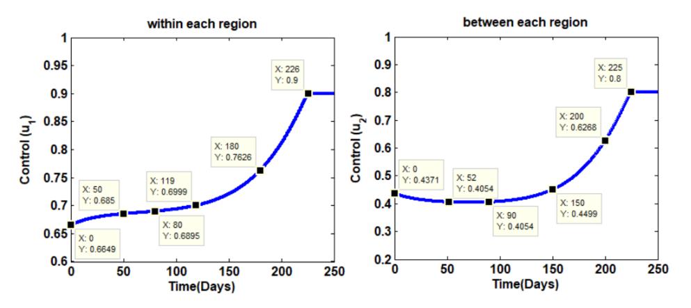
Figure 4: Behavior of the controls (x= time, y= ui values (i = 1, 2)) (w1 = 1; w2 = 1; w3 = 1; γ = 0.01; β = 0.2; m11 = 0.48; m22 = 0.22; m33 = 0.29; m12 = 0.64; m13 = 0.16; m23 = 0.19; 0.2 ⩽ u1 ⩽ 0.9; 0.1 ⩽ u2 ⩽ 0.8).
Examining the variation of u1 it was apparent that although the minimum value of mobility control between regions was 0.2 it was adequate to maintain its value at the initial point as 0.6649. Similarly, it is observed that its value varied in a short range between 0.6649 and 0.6999 from the beginning till 119 days have passed. At this point it was also perceived that from 50 days to 80 days (approximately 30 days), the difference of u1 was almost at 0.0045. Thus, it can be described as a period of the operation of lockdown restrictions. Similarly, it is observed that after 80 days, the value of u1 has increased significantly with time. Hence, after almost 80 days, the lockdown restrictions within regions should be relaxed. It also appears that u1 has reached its maximum value after 226 days. Therefore, the complete removal of the lockdown restrictions within the region has been completed after 226 days since the beginning of the execution.
Examining the variation of u2, it was clear that although the minimum value of mobility control between regions was used as 0.1, it was sufficient to maintain its value at the beginning as 0.4371. Similarly, it is observed that its value has fluctuated in a short range between 0.4371 and 0.4499 from the beginning till 150 days have passed. It is also understood that from 52 days to 90 days (approximately 38 days), the value of u2 was 0.4054 and it can be described as a period of lockdown restrictions. Correspondingly, it is detected that after 90 days the value of u2 has increased significantly with time. After almost 90 days, the lockdown restrictions between regions should be relaxed. It also appears that u2 has reached its maximum value after 225 days. Thus, the complete removal of the lockdown restrictions between the region has been completed after 225 days since the beginning.
The variation of the basic reproductive number (R0) with time is given in Figure 5. It is observed that the value of the basic reproduction number (R0) is at a high value of 21.62 with time when mobility controls were deactivated. When the mobility controls were active, the value of basic R0 was 11.15 at the beginning, and after that, basic R0 remained at a lower value than the initial value until about 120 days have passed. After that, it has undergone some upsurge; however, when the lockdown restrictions were totally removed within the region and between the regions (after 225 days have passed since the beginning), the value of basic R0 has reached 18.04. This is a value lower than basic R0 when mobility controls were deactivated.
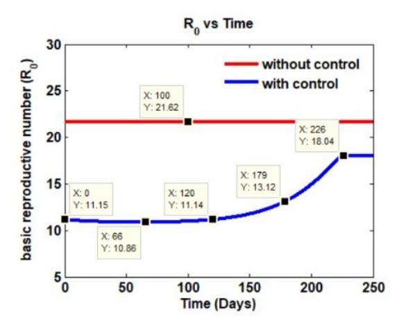
Figure 5: Behavior of the basic reproductive number (x= time , y= R0 value) (w1 = 1; w2 = 1; w3 = 1; γ = 0.01; β = 0.2; m11 = 0.48; m22 = 0.22; m33 = 0.29; m12 = 0.64; m13 = 0.16; m23 = 0.19; 0.2 ⩽ u1 ⩽ 0.9; 0.1 ⩽ u2 ⩽ 0.8).
The variation of the effective reproductive number(Rt) with time is shown in Figure 6.
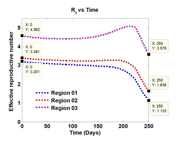
Figure 6: Behavior of the effective reproductive number (x= time , y= Rt value) (w1 = 1; w2 = 1; w3 = 1; γ = 0.01; β = 0.2; m11 = 0.48; m22 = 0.22; m33 = 0.29; m12 = 0.64; m13 = 0.16; m23 = 0.19; 0.2 ⩽ u1 ⩽ 0.9; 0.1 ⩽ u2 ⩽ 0.8).
When checking the variation of the effective reproductive number with time once the mobility controls were active, it appeared that at the beginning the effective reproductive values in the Region 01 , Region 02 and Region 03 were 3.201, 3.391, and 4.562, respectively. Effective reproductive number decreased with time in the Region 01 and Region 02 and at the end of 250 days, its values have reached a low value of 1.133 and 1.636 respectively. In the Region 03 , effective reproductive has increased slightly with time. It can be assumed that it was an outcome of its highly susceptible human proportions. Nevertheless, at the end of 250 days, its value has reached a low value of 3.579.
The variation of the the mobility controls (u1 and u2) with the weight constants (w1, w2, w3) is given in Figure 7.
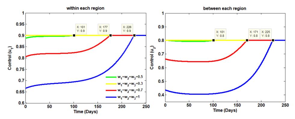
Figure 7: Behavior of the controls with the weight constants (x= time , y=ui values (i = 1, 2)) (γ = 0.01; β = 0.2; m11 = 0.48; m22 = 0.22; m33 = 0.29; m12 = 0.64; m13 = 0.16; m23 = 0.19; 0.2 ⩽ u1 ⩽ 0.9; 0.1 ⩽ u2 ⩽ 0.8).
By changing the values of the weight terms which were used to change the infected proportion in the cost function, the variation of mobility controls within and between regions was studied. It was found that when the size of the Infected proportion used in the study was reduced (that is when the values of the weight terms were reduced), the time limits were also reduced for which the lockdown restrictions ought to be imposed. Furthermore, it was also observed that it was not necessary impose lockdown restrictions once the infected proportion was identically low.
The variation of the controls with the upper bound is given in Figure 8 (the lower bound remains unchanged).
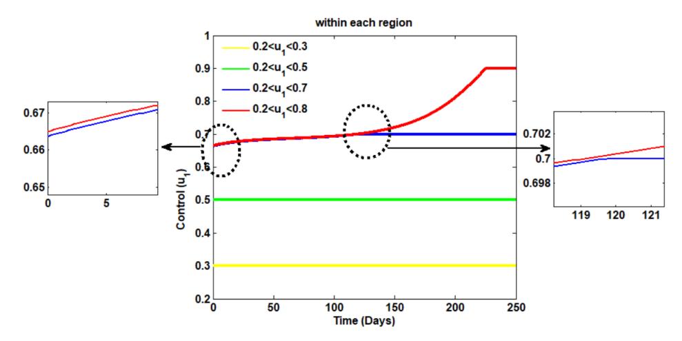
Figure 8: Behavior of the controls with the upper bound (w1 = 1; w2 = 1; w3 = 1; γ = 0.01; β = 0.2; m11 = 0.48; m22 = 0.22; m33 = 0.29; m12 = 0.64; m13 = 0.16; m23 = 0.19; 0.1 ⩽ u2 ⩽ 0.8).
Once the lower bounds of mobility controls were fixed and the maximum mobility values were reduced, it was observed that the initial values of the mobility controls also decreased. It was further observed that there was no requirement to impose lockdown restrictions when reducing the maximum values of mobility controls below a certain limit. For example, when the maximum mobility value within the region was 0.5 and
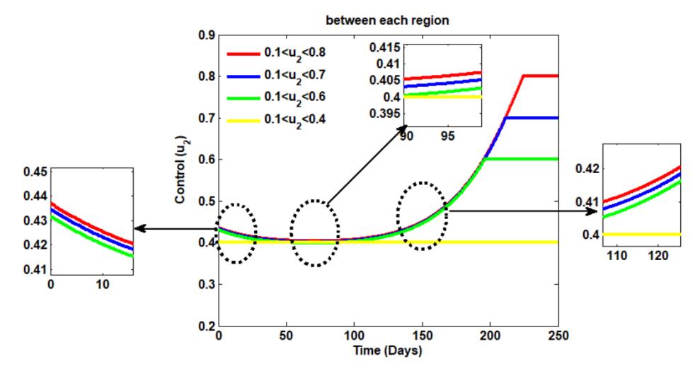
Figure 9: Behavior of the controls with the upper bound (w1 = 1; w2 = 1; w3 = 1; γ = 0.01; β = 0.2; m11 = 0.48; m22 = 0.22; m33 = 0.29; m12 = 0.64; m13 = 0.16; m23 = 0.19; 0.2 ⩽ u1 ⩽ 0.9).
the maximum mobility value between regions was 0.4, it appeared that there was no requirement to impose lockdown restrictions.
The variation of the controls with the lower bound is shown in Figure 10 (the upper bound remains unchanged).
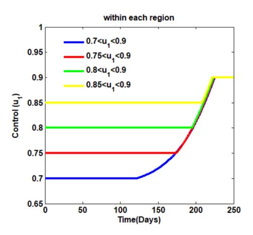
Figure 10: Behavior of the controls with the lower bound (w1 = 1; w2 = 1; w3 = 1; γ = 0.01; β = 0.2; m11 = 0.48; m22 = 0.22; m33 = 0.29; m12 = 0.64; m13 = 0.16; m23 = 0.19; 0.1 ⩽ u2 ⩽ 0.8).
Once keeping the maximum mobility values of mobility controls fixed while increasing the minimum mobility values in within the region, it was observed that the time limits required to impose lockdown restrictions should be increased. Also, it was observed that there was a variation in the same way between the regions, but when the upper bounds and lower bounds were close, it was observed that the time limits for which the lockdown limits should have been imposed decreased by a small amount.
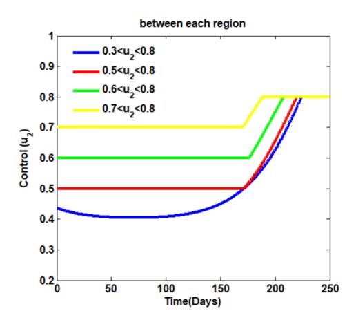
Figure 11: Behavior of the controls with the lower bound (w1 = 1; w2 = 1; w3 = 1; γ = 0.01; β = 0.2; m11 = 0.48; m22 = 0.22; m33 = 0.29; m12 = 0.64; m13 = 0.16; m23 = 0.19; 0.2 ⩽ u1 ⩽ 0.9).
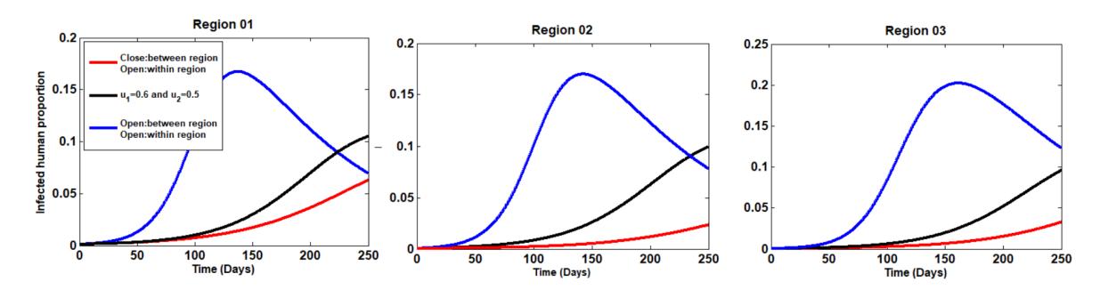
Figure 12: Behavior of the infected human proportion (w1 = 1; w2 = 1; w3 = 1; γ = 0.01; β = 0.2; m11 = 0.48; m22 = 0.22; m33 = 0.29; m12 = 0.64; m13 = 0.16; m23 = 0.19).
The variation of the infected human proportion with time is given in Figure 12. When there is no mobility restriction within and between regions, the increase in the infected human proportion occurs faster than when mobility restriction is maintained between regions. Furthermore, the rate of disease spread is lower when movement restrictions are imposed only on infected persons within and between regions than when there are no movement restrictions within and between regions. One reason for this is the emergence of new clusters of COVID-19 due to the arrival of infected people from one region to another. Another main reason can be the formation of clusters of COVID-19 due to susceptible people travelling to other regions, becoming infected with the disease, and returning to the region they came from at the end of the day. Thus, it appears that human mobility has a greater impact on the spread of COVID-19.
4. DISCUSSION
To propose ways to deficit the spread of COVID-19 in a way that minimizes the damage caused to the country's economy, in the last few years, researchers in the world, including Sri Lanka, have conducted a large amount of research based on the optimal control theory, and a large amount of research is still being conducted related to the present scenario. Thus, the researchers have proposed many mathematical models such as SIR, SEIR, etc., and have used various control variables to control the important factors (human mobility...etc.) to deficit the spread of COVID-19. Here the SIR model was designed by using two control
variables to control human mobility within(u1) and between(u2) regions to get a clear idea about how to impose a lockdown on the country and remove it.
In considering the 9-dimensional mathematical model with high-risk and low-risk exposures which was developed based on Chinese data, three control variables have been used to control the isolate possible infected cases at home(u1), nucleic acid detection ability(u2) and rational allocation of resources in the case of limited medical resources(u3) [17]. Next, it is considered the SEIR model that was designed based on data from Sri Lanka. In that case, three control variables have been used to control, the effort of personal protection such as wearing face marks(u1), measuring the rate of identifying asymptomatic cases through contact tracing, testing and isolating them to treat in designated hospitals(u2) and measures the rate of tracing, testing and isolating of patients with mild symptoms(u3) [18]. Further, a model was presented to control the spread of COVID-19 using disease-free equilibrium points as trivial equilibrium (TE), virus absenteeism equilibrium (VAE) and virus incidence equilibrium (VIE) [19]. Next, the research report, "Predictions on both the number of the first and the second waves of COVID-19 cases in Sri Lanka" has presented a SIR model [20]. Nevertheless, once studying the research related to COVID-19 and its controlling measures it is apparent that not any clear idea has been presented regarding how to apply and remove the lockdown restrictions in a way that does not harm the country's economy while systematically controlling human mobility. Nevertheless, the SIR model designed by the researchers of this study have presented a sound idea about how to apply the lockdown restrictions to save the country's economy.
In our research, Sri Lanka was divided into three main regions(three-patch) and normal human mobility rate values were calculated within and between the regions as explained in section 2.2. Hence, it is observed that the normal human mobility rate (m11) is high compared to others in Region 01 which included the districts that were the center of the spread of COVID-19 in Sri Lanka. Region 03, which represents most of the districts, has the second-highest normal human mobility rate (m33). The reason for that appears to be that the aforementioned districts contain a high job market and they are highly urbanized. Furthermore, as Region 01 contains highly urbanized districts such as Colombo, Kalutara, and Gampha, Region 01 and Regions 02 represent the highest human mobility rate value. Region 01 and Region 03 can be named as the two regions where people move in the least amounts. Moreover, in calculating the disease transmission rate, the value of m12 has been used instead of all other human mobility rate values.
Next, two control variables were used (u1, u2) to control human mobility within and between regions as explained in section 2.2. u1m11, u1m22,u1m33 have been used as the total mobility rate within the region. Moreover, u2m13, u2m12 u2m23 have been also utilized as the total mobility rate between the regions. At this point, the lockdown or relaxation is determined based on the values of u1 and u2. The value of control variables is in the range between 0 and 1, once it reaches 0, it is considered a full lockdown state and once it reaches 1, it is considered a fully open state. But to minimize the damage it causes to the economy of the country, essential services must be operated in the country. Therefore, a minimum value was always set for u1 and u2 that is not 0 and it is decided to maintain as expected. Furthermore, to control unnecessary human mobility in the country until the disease is controlled, a maximum value of u1 and u2 was maintained that is not 1.
Similarly, by changing the upper bound and lower bound values of u1 and u2, as shown in Figures 8, 9, 10 and 11 when checking the behavior of u1 and u2, it was realized that the time limits that should be imposed and the way that the lockdown should be relaxed are different for each situation. Likewise, once changing the values of the weight constants (w1, w2, w3) which were used to control the effect of I1, I2 and I3 in the cost function (Figure 7), the lockdown period which intended to be imposed and relaxed varies in each occasion.
In this research, the variation of the basic reproductive number values with time was checked under the assumption that all individuals may be infected. Nevertheless, as there are people with adequate immunity to protect themselves from the disease in a population, this research mainly carried out the variation of the effective reproductive number when the mobility controls are activated in each region to check the spread of the disease. In conducting the research, some calculations were made under various assumptions. For example, the value of the normal mobility rate between Region 01 and Region 02 (m12) and the value of the normal mobility rate between Region 02 and Region 01 (m21) are approximately equal to each other. Thus, the same assumption is used for other pairs of regions (m12 = m21, m13 = m31, m32 = m23). Similarly, it is not taken into consideration the time a person stays there after arriving in a region. Therefore, it is anticipated to continue the research without using these assumptions in the future.
5. CONCLUSION
In this research paper, the SIR model has been presented by means of two control variables and optimal control theory to control human mobility. The main objective was to provide a clear idea of how to impose lockdown rules to deficit the spread of COVID-19 and how to remove them in a way which does not degenerate the economy of the country. Thus, the data records in Sri Lanka from 2021 from April 15 to May 15 related to COVID-19 have been used [10].
According to Figure 2, the variation of the infected human proportion with and without control variables was examined. It was concluded that the rate of increase in infected proportion in all three regions with time was higher when mobility controls were deactivated than when mobility controls were activated. Furthermore, it was observed that the infected proportion increased to maximum values when the mobility controls were in the deactivated state. Nevertheless, related to those cases it was certainly apparent that the infected proportion was very low in the times when the mobility controls were activated. Also, according to Figure 4, it was observed that the lockdown limits were also being relaxed by that time. Hence, it can be concluded that once mobility controls are activated, the rate of increase in infected proportion is much lower than the deactivated mode of the mobility controls. It was also observed that when the mobility controls are activated, human mobility is at an ordinary value. It can have a strong impact on the economic security of the country.
Furthermore, some people may have immunity to protect themselves from the disease, so the average number of secondary cases per infectious case may be less than the basic reproductive number [11]. Therefore, to obtain a more definite idea about the spread of the disease, the behavior of the effective reproductive number was tested according to the time when the mobility controls were activated for the three regions. According to Figure 6, it was observed that the value of effective reproductive number has decreased with time. Consequently, it can be assumed that the spread of disease is less when mobility controls are activated.
Therefore, the behaviour of the control variables (Figures 7, 8, 9, 10, 11) was checked by changing the upper bound and lower bound of the control variables as well as the weight constants (w1, w2, w3). It can be understood that the behaviour of the control variables is successful through the occurrence of the behaviour of the control variables in a practical manner. Similarly, once examining the behaviour of control variables (Figure 7) by changing the infected proportion which was used in the cost function, it was concluded that it was more appropriate to diminish the lockdown restrictions within the region after a few days of subsequently relaxing the lockdown restrictions between regions. At this point, a full lockdown situation has not been maintained for any reason, and freedom for essential movements has been allowed. In addition, until the disease completely diminishes the country will not be fully opened.