

1. INTRODUCTION
In nature, each system element typically evolves on different time scales. We can gain insights into the system's characteristics and behavior by making assumptions about processes that operate on slower or faster time scales. This phenomenon includes chemical reactions, particle dynamics in fluids, ecological interactions, and evolutionary processes. Systems that exhibit two distinct time scales are known as fast-slow systems [7]. Fast-slow systems are widely utilized across various fields, including physics, biology, ecology, and economics. This concept helps to comprehend the dynamics of systems with two or more components that evolve at different rates.
Fast-slow systems can be examined using various methods. In 1970, Neil Fenichel introduced a geometric technique, leveraging the theory of invariant manifolds to investigate these systems, known as Geometric Singular Perturbation Theory (GSPT). GSPT provides a geometric framework for addressing problems with distinct time scale separation, explicitly aimed at analyzing fast-slow systems [7]. The fundamental concept is to simplify the system by reducing it to a lower-dimensional subsystem that is more manageable to analyze. This approach allows for the overall dynamics of the system to be studied by integrating the dynamics of each individual subsystem.
There are several articles discussing fast-slow systems and GSPT. In the article [8], Jardon et al. discuss the fast–slow framework of epidemiological models, specifically SIR, SIRS, and SIRWS. The article examines these three distinct models and offers an interpretation utilizing GSPT techniques and entry-exit functions. On the other hand, [3] examines singular perturbations in epidemiological models where transmission occurs through vectors. Numerous diseases are transmitted indirectly between humans via these vectors, which often include blood-sucking insects. These insects obtain disease-causing microorganisms by feeding on the blood of an infected host (human) and then transmitting them to a new host during their next feeding. Generally, vectors reproduce much faster than their hosts, leading to fast and slow processes within these systems.
The study of population dynamics among species within an ecosystem is essential for understanding their survival and long-term coexistence [5]. Species interactions often occur on different time scales, which can significantly impact the dynamics of the model [5]. In 1925-1926, Alfred Lotka and Vito Volterra independently addressed this phenomenon by formulating a system of differential equations to describe
*Corresponding author
Received January 11th, 2024, Revised October 18th, 2024, Accepted for publication November 15th, 2024. Copyright ©2024 Published by Indonesian Biomathematical Society, e-ISSN: 2549-2896, DOI:10.5614/cbms.2024.7.2.1
ecosystems comprising two species, one serving as the predator and the other as the prey. This framework is commonly referred to as the predator-prey model [1]. The predation process affects both species' population dynamics, helping to maintain a balance between their populations. When the prey population grows, it provides more food for the predators, leading to a subsequent increase in the predator population after a brief delay [4].
In the article by Owen and Tuwankotta [12], the dynamics of fast-slow behavior in a basic predator-prey system are examined, where neither the prey nor the predator populations have a carrying capacity. In this scenario, both populations can grow indefinitely. One of the aims is to demonstrate how the timescale parameter influences the construction of an approximation for solutions using singular perturbation techniques. They introduce a basic predator-prey model that is converted into a dimensionless form. In addition, it is assumed that the birth rate of the prey is significantly lower than the death rate of the predator.
In this research, the predator-prey model discussed in the article [12] is considered, but with the assumption that the prey population is limited. Therefore, a carrying capacity for the prey population is added to the model. The problem and primary purpose is to know how the solution behaves on the model using a geometric approach, i.e., using entry-exit functions, as done by [8].
2. PRELIMINARIES
2.1. Fast-Slow System
From a mathematical standpoint, one straightforward method to capture different time scales is employing a system of differential equations characterized by two distinct time scales, commonly referred to as a fast-slow system [9].
Definition 2.1. The (m,n)-fast-slow system is a system of differential equations that takes the form.
\[\varepsilon \frac{d\mathbf{x}}{d\tau} = \varepsilon \dot{\mathbf{x}} = \mathbf{f}(\mathbf{x}, \mathbf{y}, \varepsilon), \frac{d\mathbf{y}}{d\tau} = \dot{\mathbf{y}} = \mathbf{g}(\mathbf{x}, \mathbf{y}, \varepsilon),\] (1)
where \((\mathbf{x}, \mathbf{y}) \in \mathbb{R}^m \times \mathbb{R}^n\), \(\mathbf{f} : \mathbb{R}^m \times \mathbb{R}^n \times \mathbb{R} \to \mathbb{R}^m\), \(\mathbf{g} : \mathbb{R}^m \times \mathbb{R}^n \times \mathbb{R} \to \mathbb{R}^n\), and \(\varepsilon\), with \(0 < \varepsilon \ll 1\), is a time scale parameter. The variables \(\mathbf{x}\) are referred to as fast variables and \(\mathbf{y}\) are referred to as slow variables [9].
The parameter \(\varepsilon\), which tends towards zero and is very small, is used to differentiate the time scales between two different variables. Let \(t = \frac{\tau}{\varepsilon}\), then
\[\varepsilon \frac{d\mathbf{x}}{d\tau} = \varepsilon \frac{d\mathbf{x}}{dt} \frac{dt}{d\tau} = \varepsilon \frac{d\mathbf{x}}{dt} \frac{1}{\varepsilon} = \mathbf{x}' = \mathbf{f}(\mathbf{x}, \mathbf{y}, \varepsilon)\] and
\[\frac{d\mathbf{y}}{d\tau} = \frac{d\mathbf{y}}{dt}\frac{dt}{d\tau} = \frac{d\mathbf{y}}{dt}\frac{1}{\varepsilon} = \frac{1}{\varepsilon}\mathbf{y}' = \mathbf{g}(\mathbf{x}, \mathbf{y}, \varepsilon) \Longleftrightarrow \mathbf{y}' = \varepsilon\mathbf{g}(\mathbf{x}, \mathbf{y}, \varepsilon),\]
thus obtaining a system equivalent to the system (1) as follows:
\[\frac{d\mathbf{x}}{dt} = \mathbf{x}' = \mathbf{f}(\mathbf{x}, \mathbf{y}, \varepsilon), \frac{d\mathbf{y}}{dt} = \mathbf{y}' = \varepsilon \mathbf{g}(\mathbf{x}, \mathbf{y}, \varepsilon),\] (2)
where t being the fast time scale and dan \(\tau\) being the slow time scale. The variables \(\mathbf{x}\) and \(\mathbf{y}\) in system (2) are the updated variables \(\mathbf{x}\) and \(\mathbf{y}\) in the system (1) after time scaling. The notation \(\dot{\mathbf{x}}\) represents \(\frac{d\mathbf{x}}{d\tau}\) and \(\mathbf{x}'\) represents \(\frac{d\mathbf{x}}{dt}\).
2.2. Geometric Singular Perturbation Theory (GSPT)
The fundamental idea behind Geometric Singular Perturbation Theory (GSPT) for analyzing fast-slow systems is to investigate the singular limit cases, particularly when \(\varepsilon=0\). Subsequently, perturbation techniques are utilized to describe the dynamics of the fast-slow system [8]. This approach is anticipated to simplify the analysis of systems (1) and (2) compared to scenarios where \(\varepsilon>0\) [8]. By substituting \(\varepsilon=0\) into system (1), we derive a set of differential-algebraic equations known as the slow subsystem, which is expressed as follows:
\[\mathbf{0} = \mathbf{f}(\mathbf{x}, \mathbf{y}, 0), \dot{\mathbf{y}} = \mathbf{g}(\mathbf{x}, \mathbf{y}, 0),\] (3)
where the system (3) is the reduced problem or a differential equation with a constraint \(\mathbf{f}(\mathbf{x}, \mathbf{y}, 0) = \mathbf{0}\). The slow subsystem (3) is constrained to a critical set or critical manifold \(C_0\)
\[C_0 = \{ (\mathbf{x}, \mathbf{y}) \in \mathbb{R}^{m+n} | \mathbf{f}(\mathbf{x}, \mathbf{y}, 0) = \mathbf{0} \}.\]
Definition 2.2. A manifold is a generalization of curves and surfaces to higher dimensions. It is classified as having dimension n if all its connected components share this dimension. Specifically, a one-dimensional manifold is called a curve, a two-dimensional manifold is called a surface, and an n-dimensional manifold is known as an n-manifold [14].
It means that \(C_0\) is an m+n-manifold. Some properties of the manifold used are defined as follows:
Definition 2.3. Let \(M \subset \mathbb{R}^m\) be a connected and compact \(\mathbb{C}^k\)-manifold. Let \(\phi_t(\cdot)\) denoted trajectories of solutions of the system (1). M are called invariant manifolds if for every \(\mathbf{p} \in M\), it holds that \(\phi_t(\mathbf{p}) \in M\) for all \(t \in \mathbb{R}\). M are called local invariant manifolds if for every \(\mathbf{p} \in M\), there exists a time interval \(I_{\mathbf{p}} = (t_1, t_2)\), such that \(0 \in I_{\mathbf{p}}\) and \(\phi_t(\mathbf{p}) \in M\) for all \(t \in I_{\mathbf{p}}\) [9].
Definition 2.4. Let \(M,N \subset \mathbb{R}^m\) are an manifold-m. M and N called diffeomorphic if there exist a diffeomorfism map, i.e. the map \(\mathcal{F}: M \to N\) that has inverse \(\mathcal{F}^{-1}: N \to M\), where \(\mathcal{F}\) and \(\mathcal{F}^{-1}\) both are \(\mathcal{C}^k\) functions [14].
When \(\varepsilon = 0\) is substitute to the system (2), we obtained the parameterized system of differential equation called fast subsystem, i.e.
\[\mathbf{x}' = \mathbf{f}(\mathbf{x}, \mathbf{y}, 0), \mathbf{y}' = \mathbf{0},\](4)
where the system (4) is also called layer equation or layer problem [9]. The relationship between equilibrium points of the fast subsystem (4) and the critical manifold \(C_0\), i.e.
Proposition 2.1. Equilibrium points of the fast subsystem (4) are in one-to-one correspondence with points in \(C_0\) [9].
Proof: Let us consider any value \(\mathbf{y} = \mathbf{y}_0\). If \(\mathbf{x}_0\) is an equilibrium point of the fast flow \(\mathbf{x}' = \mathbf{f}(\mathbf{x}, \mathbf{y}_0, 0)\), then \(\mathbf{f}(\mathbf{x}_0, \mathbf{y}_0, 0) = 0\), and it can be concluded that \((\mathbf{x}_0, \mathbf{y}_0) \in C_0\). Similarly, the reverse is also true.
The bases of GSPT is the Fenichel's theorem, which requires certain assumptions about \(C_0\). Specifically, it is assumed that there is a compact submanifold S of dimension n (or with a boundary), contained in \(C_0\) [8]. Consider the (m, n)-fast-slow system (1), with the functions \(\mathbf{f}\) and \(\mathbf{g}\) being sufficiently smooth [9].
Definition 2.5. Let \(S \subset C_0\). Submanifold S is said to be normally hyperbolic if for all \(\mathbf{p} \in S\), the \(m \times m\) matrix \((D_{\mathbf{x}}\mathbf{f})(\mathbf{p},0)\) has no eigenvalues with real part equal to zero [9].
Definition 2.6. Let \(S \subset C_0\) be normally hyperbolic. If all eigenvalues of \((D_{\mathbf{x}}\mathbf{f})(\mathbf{p},0)\) have negative real parts, then S is called attracting. If all eigenvalues of \((D_{\mathbf{x}}\mathbf{f})(\mathbf{p},0)\) have positive real parts, then S is called repelling, and if otherwise, S is of saddle type [9].
For the next theorem, the definition of Hausdorff distance is required:
Definition 2.7. Let \(U, V \subset \mathbb{R}^m\) be manifolds. The Hausdorff distance between U and V is defined as
\[d_H(U,V) = \max \Big\{ \max_{u \in U} \min_{v \in V} d(u,v), \max_{v \in V} \min_{u \in U} d(u,v) \Big\},\] where d(u, v) is the distance between u and v [9].
Theorem 2.1. [9] Suppose \(S = S_0 \subset C_0\) is a compact normally hyperbolic submanifold of the critical manifold \(C_0\) of (1) and that \(f, g \in C^r\) \((r < \infty)\), then for \(\varepsilon > 0\) sufficiently small, the following hold:
- (i) There exist a locally invariant manifold \(S_{\varepsilon}\) that diffeomorphic to \(S_0\).
- (ii) As \(\varepsilon \to 0\), \(S_{\varepsilon}\) has Hausdorff distance of order \(\mathcal{O}(\varepsilon)\) from \(S_0\), and the flow on \(S_{\varepsilon}\) converges to the slow flow
- (iii) \(S_{\varepsilon}\) is \(C^r\)-smooth.
- (iv) \(S_{\varepsilon}\) is normally hyperbolic and has the same stability properties with respect to the fast variables as \(S_0\).
(v) \(S_{\varepsilon}\) is usually not unique.
The manifold \(S_{\varepsilon}\) is known as the slow manifold. All distinct slow manifolds \(S_{\varepsilon}\) are closely aligned, exhibiting a proximity characterized by an order of \(\mathcal{O}(\varepsilon^{-\xi/\varepsilon})\), for some \(\xi > 0\). Consequently, the selection of \(S_{\varepsilon}\) does not significantly impact the overall analysis or the numerical results obtained [8].
2.3. Entry-Exit Function
One of the GSPT methods for establishing the relationship between fast and slow flow. This function yields a version of the Poincaré mapping between two regions of the phase space, allowing for an approximation of the trajectory behavior around points on the critical manifold where stability shifts (from attracting to repelling) [8].
Definition 2.8. Consider an n-dimensional system given by \(\mathbf{x}' = \mathbf{f}(\mathbf{x})\). Let \(\Sigma\) represent (n-1)-dimensional surface of section. The Poincaré Mapping \(\Pi\) is defined as a mapping from \(\Sigma\) back to itself. If \(\mathbf{x}_i \in \Sigma\) denotes the i-th intersection of the trajectory with the surface, then the Poincaré mapping is defined as
\[\mathbf{x}_{i+1} = \Pi(\mathbf{x}_i).\] and the illustration is shown in the Figure 1 below
Figure 1: Sketch of the Poincaré mapping [13].
Let \(\mathbf{x}^*\) be an equilibrium point of \(\Pi\), i.e., \(\Pi(\mathbf{x}^*) = \mathbf{x}^*\), then trajectories starting from the point \(\mathbf{x}^*\) return to \(\mathbf{x}^*\) and form homoclinic trajectories of the system \(\mathbf{x} = \mathbf{f}(\mathbf{x})\) [13].
Consider the (1,1)-fast-slow system in the form
\[\begin{aligned} x' &= x u(x, y, \varepsilon), \\ y' &= \varepsilon v(x, y, \varepsilon), \end{aligned} \tag{5}\] with \((x,y) \in \mathbb{R}^2\), v(0,y,0) > 0, and u(0,y,0) < 0 for \(y \in C^-\), and u(0,y,0) > 0 for \(y \in C^+\). Here, \(C^{-} = \{(x,y) \in \mathbb{R}^2 | x = 0 \text{ and } 0 < y < \tilde{y}\}, \text{ and } C^{+} = \{(x,y) \in \mathbb{R}^2 | x = 0 \text{ and } y > \tilde{y}\}, \text{ where } \tilde{y} \text{ is the } \tilde{y} \in \mathbb{R}^2\)ordinate of the point on the critical manifold where stability changes.
When \(\varepsilon = 0\), the y-axis contains equilibrium points of the slow subsystem from (6), which are given by
\[0 = x u(x, y, \varepsilon), y' = v(x, y, \varepsilon),\] (6)
resulting in the critical manifold \(C_0=\{(x,y)\in\mathbb{R}^2|x=0 \text{ or } u(x,y,\varepsilon)=0\}\). These equilibria are normally attracting for \(y \in C^-\) because \(D_x(xu(x,y,\varepsilon))|_{C^-} < 0\) and normally repelling for \(y \in C^+\) because \(D_x(xu(x,y,\varepsilon))|_{C^+} > 0\) (using Definition 2.6), with \(C^- \cup C^+ \subset C_0\).
When \(\varepsilon > 0\), if the solution starts at \((x_0, y_0)\) with \(x_0 > 0\) and \(y_0 \in C^-\), the solution will quickly approach the y-axis because \(C^-\) is attracting. When the solution is close enough to the y-axis, meaning \(\varepsilon \to 0\) and \(x \to 0\),
\[\frac{dx}{dy} = \frac{x u(x, y, \varepsilon)}{\varepsilon v(x, y, \varepsilon)} \to \frac{u(0, y, 0)}{v(0, y, 0)} < 0,\] then the solution will move upward along the y-axis and gradually move away from the y-axis because \(C^+\) is repelling. Therefore, the solution will intersect the line \(x=x_0\) at a point with y-coordinate denoted as \(p_{\varepsilon}(y_0)\). The visualization can be seen in Figure 2.
Figure 2: Visualization of the entry-exit mapping on the line \(x = x_0\). The blue-colored line segment represents \(C^-\), and the red-colored segment represents \(C^+\).
To achieve the balancing, from the system (6), the limit of the gradient of the tangent lines of the solution approaching zero can be used, which is expressed as
\[\int_{y_0}^{p_{\varepsilon}(y_0)} \frac{dx}{dy} \, dy = \int_{y_0}^{p_{\varepsilon}(y_0)} \frac{u(x, y, \varepsilon)}{v(x, y, \varepsilon)} \, dy = 0. \tag{7}\]
When \(\varepsilon \to 0\) and \(x_0 = \mathcal{O}(\varepsilon)\), then \(x_0 \to 0\), so \(p_{\varepsilon}(y_0)\) approaches the function \(p_0(y_0)\), given implicitly as
\[\int_{y_0}^{p_0(y_0)} \frac{u(0, y, 0)}{v(0, y, 0)} \, dy = 0.\] (8)
3. MODEL FORMULATION
The model employed is a basic predator-prey model in [12], with slight modifications to incorporate the assumption that the birth rate of the prey is significantly lower than the death rate of the predator. It also assumes a limited prey population, indicating that the prey population grows logistically. Let p and q denote the predator and prey population densities at time t, respectively. The system of ordinary differential equations that describes the simple predation process with a constrained prey population is expressed as follows:
\[\frac{dp}{dt} = p(\beta q - \gamma), \frac{dq}{dt} = \alpha q \left(1 - \frac{q}{K}\right) - \beta p q,\] (9)
where \(\alpha\) is the prey birth rate, \(\gamma\) is the predator death rate, and \(\beta\) is the predation rate. The variables \(p, q, \alpha, \beta, \gamma\) are all positive. And the detail about all variables and parameters see Table 1.
| Variables and Parameters | Dimensions |
|---|---|
| p | [population dimension] |
| \(\overline{q}\) | [population dimension] |
| \(\alpha\) | 1 [time] |
| \(\gamma\) | 1 [time] |
| \(\beta\) | [population dimension][time] |
| K | [population dimension] |
Table 1: Variables and parameters along with dimensions of the predator-prey model (9).
To simplify the analysis without the dimension of each variable and parameter, the system (9) is transformed into a dimensionless form by introducing the substitutions \(x = \frac{\beta}{\alpha}p\), \(y = \frac{1}{K}q\), and \(\tilde{t} = \gamma t\). Simplifying further by removing the tilde notation, the system (9) can be written as follows:
\[\frac{dx}{dt} = x' = x(\eta y - 1), \frac{dy}{dt} = y' = \varepsilon y(1 - x - y),\] (10)
where, \(\varepsilon = \frac{\alpha}{\gamma} \ll 1\), \(\eta = \frac{\beta K}{\gamma}\), and using the transformation \(\tau = \varepsilon t\), the equivalent system is obtained:
\[\varepsilon \frac{dx}{d\tau} = \varepsilon \dot{x} = x (\eta y - 1), \frac{dy}{d\tau} = \dot{y} = y(1 - x - y),\] (11)
where, t represents the fast time scale, and \(\tau\) represents the slow time scale. The functions in the form of the system (2) are \(f(x,y,\varepsilon)=x(\eta y-1)\) and \(g(x,y,\varepsilon)=y(1-x-y)\).
4. MODEL ANALYSIS
The predator-prey model in the form of the fast-slow system that has been presented will be analyzed as follows:
4.1. The existence of equilibrium points
In analyzing the dynamic system (10), the initial step is to identify the equilibrium points. To determine the equilibrium points of the system (10), we solve the system of equations given by setting the right-hand sides of the equations equal to zero. This involves finding the values of the variables that satisfy the following conditions
\[x(\eta y - 1) = 0, (12a)\]
\[\varepsilon y(1-x-y) = 0. \tag{12b}\]
From Equation (12a), we find that x=0 or \(y=\frac{1}{\eta}\). From Equation (12b), we derive y=0 or y=1-x. This leads us to three equilibrium points:
- 1. \(E_0 = (0,0)\). This point indicates the absence of both prey and predator populations, signifying extinction,
- 2. \(E_1 = (0,1)\). Here, the prey population is at its carrying capacity K, while the predator population becomes extinct, as its death rate is lower than the predation rate, and
- 3. \(E_2 = \left(1 \frac{1}{\eta}, \frac{1}{\eta}\right)\). This point represents a coexistence equilibrium, where both prey and predator populations exist at specific levels. Since populations must be positive, we require \(1 \frac{1}{\eta} > 0\), which implies that \(\eta > 1\) for \(E_2\) to exist.
4.2. GSPT analysis on Model
To analyze when \(\varepsilon > 0\), we consider the singular limit case \(\varepsilon = 0\) for the system (11), resulting in the slow subsystem
\[0 = x (\eta y - 1), \dot{y} = y(1 - x - y),\] (13)
where the critical manifold is the set
\[C_0 = \{(x, y) \in \mathbb{R}^2 | x(\eta y - 1) = 0 \}\] and for the system (10), we obtain the fast subsystem
\[x' = x (\eta y - 1),\]
\(y' = 0.\) (14)
The equilibrium points of the slow subsystem (13) are \((x^*, y^*) = (0, 0)\) and \((x^*, y^*) = (0, 1)\). The fast flow along \(C_0\) is given by \(\dot{y} = y(1 - x - y)\). Based on Definition 2.5, Definition 2.6, and Proposition 2.1, a submanifold of \(C_0\) is defined as hyperbolic normal, i.e.
\[\begin{split} C_0^- &= \left\{ (x,y) \in \mathbb{R}^2 | x = 0 \text{ and } 0 < y < \frac{1}{\eta} \right\} \quad \text{ and } \\ C_0^+ &= \left\{ (x,y) \in \mathbb{R}^2 | x = 0 \text{ and } y > \frac{1}{\eta} \right\}. \end{split}\]
Therefore, \((D_x f)(x,y,0)|_{C_0^-} < 0\), making \(C_0^-\) attracting, and \((D_x f)(x,y,0)|_{C_0^+} > 0\), making \(C_0^+\) repelling, with a loss of normally hyperbolicity at \(y = \frac{1}{\eta}\). All of these are illustrated in Figure 3.
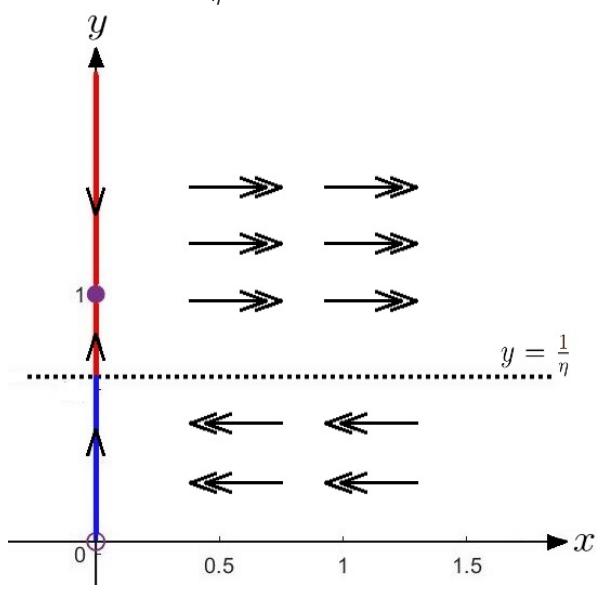
Figure 3: Fast and slow flow diagram. Single arrows: slow flow, and double arrows: fast flow. Blue line segment: stable manifold \(C_0^-\), and red line segment: unstable manifold \(C_0^+\).
Next, we determine the trajectories of the layer equation (fast subsystem (14)). From Figure 3, it can be observed that if the initial point is at (x,y) with x>0 and \(y>\frac{1}{\eta}\), its trajectory moves away from \(C_0^+\) towards infinity. To obtain the constant of motion describing the trajectory of (14) at a relatively large value of x, i.e. \(x=\frac{\tilde{x}}{\varepsilon}\), the system (10) can be written as:
\[\tilde{x}' = \tilde{x} (\eta y - 1), y' = \varepsilon y (1 - y) - \tilde{x} y,\] (15)
Thus, when \(\varepsilon = 0\) is substituted into (15), the fast subsystem (14) becomes
\[\tilde{x}' = \tilde{x} (\eta y - 1), y' = -\tilde{x} y.\] (16)
From the system (16) obtained the constant of motion for (14) is \(\Gamma(\tilde{x}, y) = \eta y - \ln(y) + \tilde{x}\), which describes the trajectory of the layer equation (16).
4.3. Applying the Entry-Exit Function to the Model
Next, we determine the relationship between fast and slow flow or vice versa. By using the entry-exit formula, the behavior of trajectories around the normal non-hyperbolic point \((x,y)=(0,\frac{1}{\eta})\) can be explained. Based on the form of (6), from the system (10), where \(u(0,y,0)=\eta y-1\) and v(0,y,0)=y(1-y), when \(x_0>0\) and \(y\in(0,1),\) v(0,y,0)>0. Also, for \(y\in\left(0,\frac{1}{\eta}\right),\) u(0,y,0)<0, and for \(y\in\left(\frac{1}{\eta},1\right),\) u(0,y,0)>0. Therefore, the entry-exit formula can be applied by implementing the integral equation (8). This yields \(p_0(y_0)\), which is a positive root of the equation
\[\int_{y_0}^{p_0(y_0)} \frac{\eta y - 1}{y(1 - y)} dy = 0,\] \[(\eta - 1) \ln \left( \frac{1 - y_0}{1 - p_0(y_0)} \right) + \ln \left( \frac{y_0}{p_0(y_0)} \right) = 0.\] (17)
Let us consider a mapping
\[\Pi_1: \mathbb{R} \times \left(\frac{1}{\eta}, 1\right) \to \mathbb{R} \times \left(0, \frac{1}{\eta}\right).\]
and
\[\Pi_2: \mathbb{R} \times \left(0, \frac{1}{\eta}\right) \to \mathbb{R} \times \left(\frac{1}{\eta}, 1\right),\] as illustrated in Figure 4.
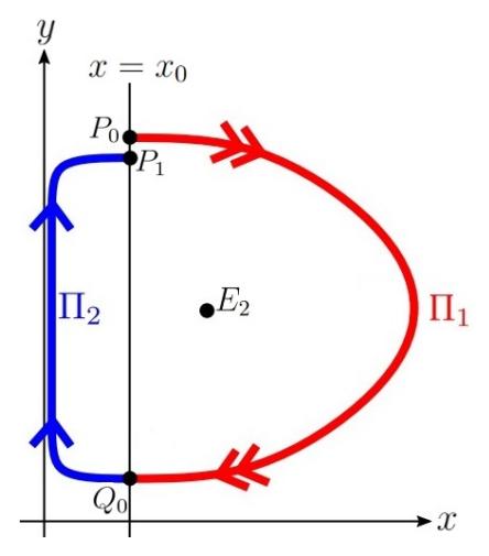
Figure 4: Sketch of \(\Pi_1\) and \(\Pi_2\).
Examining the composition of \(\Pi_1\) and \(\Pi_2\) provides a Poincaré mapping
\[\Pi: A \to B,\] where A = n (x, y) ∈ R 2 |x = x0, y ∈ [yE2 , 1)o and B = n (x, y) ∈ R 2 |x = x0, Π2(Π1(y)) ∈ [yE2 , 1)o . With Σ = {(x, y)|x = x0} is the 1-dimensional surface of section. Thus, starting from the point P0 ∈ Σ, this composition will map it to P1 ∈ Σ.
As a notation, let us define Q0 = Π1(P0) and P1 = Π2(Q0). Then, Equation (17) can be written as:
\[(\eta - 1) \ln \left( \frac{1 - Q_0}{1 - y} \right) + \ln \left( \frac{Q_0}{y} \right) = 0.\]
P1 is the exit point, which is a positive root greater than Q0, of the function
\[F(y; Q_0) = (1 - \eta) \ln \left( \frac{1 - Q_0}{1 - y} \right) - \ln \left( \frac{Q_0}{y} \right).\]
In other words, Pi+1 is a positive root of F(y; Qi) = 0, for i = 0, 1, 2, . . . , then we obtain
\[y(1-y)^{\eta-1} - Q_i(1-Q_i)^{\eta-1} = 0. (18)\]
Equation (18) can be expanded into the polynomial form using binomial expansion, i.e.
\[\begin{cases} y \sum_{i=0}^{\eta-1} \frac{(\eta-1)!}{i!(\eta-1-i)!} (-y)^i - Q_i (1-Q_i)^{\eta-1} = 0, & (\eta > 1) \in \mathbb{Z}, \\ y \sum_{i=0}^{\infty} \frac{(\eta-1)!}{i!(\eta-1-i)!} (-y)^i - Q_i (1-Q_i)^{\eta-1} = 0, & (\eta > 1) \in \mathbb{R}. \end{cases}\] (19)
Note that Π(P0) < P0 if and only if Π2(Q0) < Π −1 1 (Q0). Based on Γ(x0, y) = Γ(x0, P0), then Π −1 1 (Qi) > Qi is a root of the function
\[G(y; P_i) = \eta(y - P_i) + \ln\left(\frac{P_i}{y}\right).\]
In other words, Qi is a positive root of G(y; Pi) = 0, for i = 0, 1, 2, · · · , then we obtain
\[y = -\frac{1}{\eta}W\left[-\eta P_i e^{-\eta P_i}\right]. \tag{20}\] where W[.] is the Lambert W function. Using the properties of W[.], then the value of Qi is given by
\[Q_{i} = \frac{1}{\eta} W_{-1} \left[ -\eta P_{i} e^{-\eta P_{i}} \right]. \tag{21}\]
Based on the functions F(y; Qi) and G(y; Pi), we obtain a sequence that converges to 1 η , i.e.
\[P_0, P_1 = \Pi_2(Q_0), \dots, P_i = \Pi_2(Q_{i-1}), \tag{22}\]
and
\[Q_0 = \Pi_1(P_0), Q_1 = \Pi_1(P_1), \dots, Q_i = \Pi_1(P_i).\] (23)
Proposition 4.1. The sequences {Pi} and {Qi}, given by (22) and (23), both converge to 1 η .
Proof: It is known that the sequence Pi can be obtained from the equation (18), which is
\[y(1-y)^{\eta-1} - c(Q_i) = 0, (24)\]
with c(Qi) = Qi(1 − Qi) η−1 , and Pi+1 is a positive root of (24) that is greater than Qi . The monotonicity of c(Qi) can be determined using its derivative set to zero, i.e.,
\[\begin{split} \frac{dc(Q_i)}{dQ_i} &= 0, \\ (1-Q_i)^{\eta-1} - (\eta-1)Q_i(1-Q_i)^{\eta-2} &= 0, \\ (1-Q_i)^{\eta-1} \left(1 - (\eta-1)Q_i(1-Q_i)^{-1}\right) &= 0, \end{split}\]
resulting in \(Q_i=1\) or \(Q_i=\frac{1}{\eta}\). Thus, in the interval \(Q_i<\frac{1}{\eta}\), the function \(c(Q_i)\) is monotonically increasing, in the interval \(\frac{1}{\eta}< Q_i<1\), it is monotonically decreasing, and in the interval \(Q_i>1\), it increases when \(\eta\) is odd and decreases when \(\eta\) is even, so \(c(Q_i)\leq \frac{1}{\eta}\). Using the same property, \(y(1-y)^{\eta-1}\) is monotonically increasing in the interval \(0< y<\frac{1}{\eta}\) and monotonically decreasing in the interval \(\frac{1}{\eta}< y<1\). In other words, the graph of \(y(1-y)^{\eta-1}\) opens downwards in the interval 0< y<1. Since \(P_{i+1}\) is a root of (24), then
\[P_{i+1}(1 - P_{i+1})^{\eta - 1} - c(Q_i) = 0,\]
Choose \(Q_a,Q_b\in\left(0,\frac{1}{\eta}\right)\), with \(Q_b>Q_a\). When \(c(Q_i)\) is monotonically increasing, the graph of \(P_{i+1}(1-P_{i+1})^{\eta-1}-c(Q_i)\) is a shift of the graph of \(P_{i+1}(1-P_{i+1})^{\eta-1}\) downward by \(c(Q_i)\). This means \(P_{i+1}=P_b< P_a\). And due to the monotonicity property of \(y(1-y)^{\eta-1}, P_i\) is bounded below by \(\frac{1}{\eta}\). Therefore, since \(P_i\) is bounded below and monotonically decreasing, it is proved that the sequence \(P_i\) converges to \(\frac{1}{\eta}\). Next, for the sequence \(Q_i\) obtained from Equation (21), to prove the convergence of \(Q_i\), we can easily use the limit, i.e
\[\lim_{i \to \infty} Q_i = \lim_{i \to \infty} \left( -\frac{1}{\eta} W_{-1} [-\eta P_i e^{-\eta P_i}] \right).\]
Since \(P_i\) converges to \(\frac{1}{n}\), then
\[\lim_{i \to \infty} \left( -\frac{1}{\eta} W_{-1} \left[ -\eta P_i e^{-\eta P_i} \right] \right) = -\frac{1}{\eta} W_{-1} \left[ -\eta \frac{1}{\eta} e^{-\eta \frac{1}{\eta}} \right] = -\frac{1}{\eta} W_{-1} \left[ -e^{-1} \right] = \frac{1}{\eta}.\]
Thus, it is proven that the sequence \(Q_i\) converges to \(\frac{1}{\eta}\).
4.4. Fast-Slow Structure conditions
According to Proposition 4.1 and the monotonicity property of the function G, each trajectory of the solution to the system (10) when \(y=\frac{1}{\eta}\) indicates that the value of x reaches a minimum at \(x_{\min}=\mathcal{O}(\varepsilon)=\varepsilon\mathcal{K}\), where \(\mathcal{K}>0\) is a constant. Next, we will determine the conditions for the distance between the initial point and the point \(E_2\) using the singular perturbation technique, as done by [12]. Let x=X and \(\eta y-1=\varepsilon^\sigma Y\), obtained
\[X' = \varepsilon^{\sigma} XY,\] \[Y' = \varepsilon^{1-\sigma} (\varepsilon^{\sigma} Y + 1) \left( 1 - X - \frac{1}{\eta} (\varepsilon^{\sigma} Y + 1) \right).\] (25)
Choose \(\sigma = 0.5\), and let \(\varepsilon^{0.5} = \mu\). Thus, the system (25) can be written as
\[X' = \mu XY, Y' = \mu (1 + \mu Y) \left( 1 - X - \frac{1}{\eta} (\mu Y + 1) \right).\] (26)
With the scaling \(\tau = \mu t\), the system (26) becomes
\[\dot{X} = XY,\] \(\dot{Y} = (1 + \mu Y) \left( 1 - X - \frac{1}{\eta} (\mu Y + 1) \right).\) (27)
Then, as \(\varepsilon \to 0\), \(\mu \to 0\), and the system (27) becomes
\[\dot{X} = XY,\] \(\dot{Y} = 1 - \frac{1}{\eta} - X.\) (28)
From (28) we get
\[\Phi(x_0, y_0) = \left(1 - \frac{1}{\eta}\right) \ln\left(\frac{x_0}{\varepsilon \mathcal{K}}\right) - x_0 - \frac{1}{2\varepsilon} (\eta y_0 - 1)^2 + \varepsilon \mathcal{K} = 0.\] (29)
The curve \(\Phi(x_0, y_0) = 0\) represents the boundary of the initial values for which the solutions of the system (10) exhibit a fast-slow structure.
5. SIMULATION
In the analysis results using GSPT, it is obtained that the equilibrium points are stable with global asymptotic stability when \(\eta > 1\), and two converging sequences are formed towards a single value, namely \(\frac{1}{\eta}\). As an illustration, let us determine the values of \(P_i\) and \(Q_i\) with \(\eta = 2\). Given the known value of \(P_0\), from Equation (21), we obtain that \(Q_i\) is
\[Q_{i} = -\frac{1}{n}W_{0}\left[-2P_{i}e^{-2P_{i}}\right].\]
The value of \(Q_i\) is then used to determine the value of \(P_{i+1}\) using Equation (19), which is
\[y(1-y) - Q_i(1-Q_i) = 0,\]
\[y^2 - y + Q_i(1-Q_i) = 0,\]
(30)
so the values of y that satisfy the equation are \(y = \frac{1 \pm (2Q_i - 1)}{2}\), namely \(y = Q_i\) or \(y = 1 - Q_i\), and thus \(P_{i+1} = 1 - Q_i\).
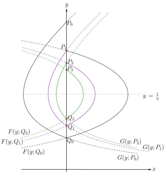
Figure 5: Graphs of functions \(F(y; Q_i)\) and \(G(y; P_i)\) for \(\eta = 2\) and \(P_0 = 0.98\).
The numerical results using Wolfram Mathematica can be seen in Table 2, where the values of \(P_i\) and \(Q_i\) converge to the value 0.5.
Table 2: Values of \(P_i\) and \(Q_i\) up to the \(100^{th}\) iteration, with \(\eta = 2\) and \(P_0 = 0.98\).
| i | \(P_i\) | \(Q_i\) | i | \(P_i\) | \(Q_i\) |
|---|---|---|---|---|---|
| 0 | 0.98 | 0.210161 | |||
| 1 | 0.789839 | 0.291578 | : | : | : |
| 2 | 0.708422 | 0.337117 | 90 | 0.508186 | 0.491903 |
| 3 | 0.662883 | 0.366272 | 91 | 0.508097 | 0.491989 |
| 4 | 0.633728 | 0.386555 | 92 | 0.508011 | 0.492074 |
| 5 | 0.613445 | 0.401486 | 93 | 0.507926 | 0.492157 |
| 6 | 0.598514 | 0.412939 | 94 | 0.507843 | 0.492238 |
| 7 | 0.587061 | 0.422004 | 95 | 0.507762 | 0.492318 |
| 8 | 0.577996 | 0.429357 | 96 | 0.507682 | 0.492395 |
| 9 | 0.570643 | 0.435443 | 97 | 0.507605 | 0.492472 |
| 10 | 0.564557 | 0.440563 | 98 | 0.507528 | 0.492547 |
| 99 | 0.507453 | 0.492620 | |||
| : | : | : | 100 | 0.507380 | 0.492692 |
To verify the analysis results using GSPT, a stability analysis of equilibrium points is conducted. First, the Jacobian matrix of the system (10) is determined, which is
\[J(x,y) = \begin{pmatrix} \frac{\partial f(x,y,\varepsilon)}{\partial x} & \frac{\partial f(x,y,\varepsilon)}{\partial y} \\ \frac{\partial g(x,y,\varepsilon)}{\partial x} & \frac{\partial g(x,y,\varepsilon)}{\partial y} \end{pmatrix} = \begin{pmatrix} \eta y - 1 & \eta x \\ -\varepsilon y & \varepsilon (1-x-2y) \end{pmatrix}.\]
For \(E_0\), its Jacobian matrix is
\[J(E_0) = J(0,0) = \begin{pmatrix} -1 & 0 \\ 0 & \varepsilon \end{pmatrix},\] which has eigenvalues \(\lambda_1 = -1 < 0\) and \(\lambda_2 = \varepsilon > 0\). The stability type is a saddle point. The matrix \(J(E_0)\) also has a determinant value of \(\det(J(E_0)) = -\varepsilon < 0\). We know that the stability type of the point \(E_0\) is also unstable (saddle point). For \(E_1\), its Jacobian matrix is
\[J(E_1) = J(0,1) = \begin{pmatrix} \eta - 1 & 0 \\ -\varepsilon & -\varepsilon \end{pmatrix},\] which has eigenvalues \(\lambda_1 = \eta - 1\) and \(\lambda_2 = -\varepsilon < 0\). When \(\eta < 1\), the type of stability is a stable node, and when \(\eta > 1\), it is a saddle point. The matrix \(J(E_1)\) also has a determinant value of \(\det(J(E_1)) = -\varepsilon(\eta - 1)\) and a trace value of \(trace(J(E_1)) = (\eta - 1) - \varepsilon\). Therefore, the stability is also as follows.
Table 3: Stability of point \(E_1\).
| Value of \(\eta\) | \(trace(J(E_1))\) or \((r)\) | \[\det(J(E_1))\] (s) | Value of \(r^2 - 4s\) | Stability Type |
|---|---|---|---|---|
| < 1 | < 0 | > 0 | > 0 | Stable (stable node) |
| > 1 | Indeterminate | < 0 | < 0 | Unstable (saddle point) |
For \(E_2\), its Jacobian matrix is
\[J(E_2) = J(1 - \frac{1}{\eta}, \frac{1}{\eta}) = \begin{pmatrix} 0 & \eta - 1 \\ -\frac{\varepsilon}{\eta} & -\frac{\varepsilon}{\eta} \end{pmatrix},\] which has eigenvalues \(\lambda_{1,2}=\frac{-\varepsilon\pm\sqrt{\varepsilon^2-4\varepsilon\eta(\eta-1)}}{2\eta}\). When \(\eta<1\), the values of \(\lambda_1\) and \(\lambda_2\) are real and have opposite signs, so the stability type is a saddle point. When \(1<\eta<\frac{2+\sqrt{4+\varepsilon}}{4}\), the values of \(\lambda_{1,2}\) are negative, making the stability type a stable node. Finally, when \(\eta>\frac{2+\sqrt{4+\varepsilon}}{4}\), the values of \(\lambda_{1,2}\) become complex, with \(\mu=-\frac{\varepsilon}{2\eta}<0\), leading to a stable spiral stability type. The matrix \(J(E_2)\) also has determinant value \(\det(J(E_2))=\frac{\varepsilon}{\eta}(\eta-1)\) and trace value \(trace(J(E_2))=-\frac{\varepsilon}{\eta}\). Therefore, for simplicity we write \(\frac{2+\sqrt{4+\varepsilon}}{4}=\eta_0\), then the stability is also presented in Table 4.
Based on the calculations above, the phase portraits of the system (10) are illustrated in Figure 6. For certain initial values, when \(\eta < 1\), the solution's trajectories converge towards the point \(E_1\), and when \(\eta > 1\), the solution trajectories converge towards the point \(E_2\). (Note: Magenta points represent equilibrium points, with filled points indicating stable equilibrium and unfilled points indicating unstable equilibrium). In Figure 6a and Figure 6b, the parameter values used is \(\varepsilon = 1\).
In Figure 6a, solution trajectories, when x < 0 and for certain y, tend to approach the point \(E_2\) but then are attracted to point \(E_1\), and some move away from \(E_2\) over time. When x > 0 and y > 0, trajectories tend to approach the point \(E_0\) and then are attracted to point \(E_2\). In Figure 6b, solution trajectories do not converge
Table 4: Stability of point \(E_2\).
| Value of \(\eta\) | \(trace(J(E_2))\) | \[\det(J(E_2))\] (s) | \(r^2 - 4s\) | Stability Type |
|---|---|---|---|---|
| < 1 | < 0 | < 0 | > 0 | Unstable (saddle point) |
| \(> 1\) and \(< \eta_0\) | < 0 | > 0 | > 0 | Stable (stable node) |
| \(> \eta_0\) | < 0 | > 0 | < 0 | Stable (stable spiral) |
to any equilibrium point when x < 0 and y > 0, and also when x > 0 and y > 0, solution trajectories spiral towards point \(E_2\).
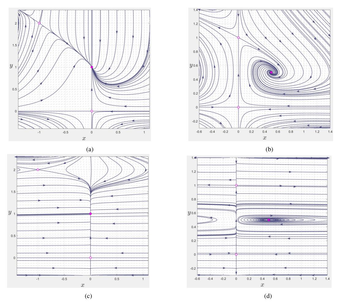
Figure 6: Phase portraits when \(\varepsilon=1\), (a) when \(\eta=0.5\), and (b) when \(\eta=2\), as well as when \(\varepsilon=0.01\), (c) when \(\eta=0.5\), and (d) when \(\eta=2\). The magenta-colored points represent equilibrium points. Filled points indicate stable equilibrium, while unfilled points indicate unstable equilibrium.
However, for a population considered only in quadrant I, it can be observed that when \(\eta < 1\), solution trajectories converge to point \(E_1 = (0,1)\). This implies that the predator population will decrease because the predation rate is smaller than the predator death rate. Eventually, there will be a point of extinction. Due to the initial assumption \(y = \frac{1}{K}q\), the prey population will reach the carrying capacity K. When \(\eta > 1\), solution trajectories converge to point \(E_2 = \left(1 - \frac{1}{\eta}, \frac{1}{\eta}\right)\). This implies that the predator and prey populations will grow alternately and approach the same level, which is \(\frac{1}{2}\).
For Figure 6c and Figure 6d, the values used are \(\varepsilon=0.01\). On Figure 6c, the behavior of the solution trajectories is similar to Figure 6a, where for certain values of x<0 and y, trajectories tend to approach the point \(E_2\) but then are attracted to point \(E_1\). Some trajectories move away from \(E_2\) throughout the time. When x>0 and y>0, trajectories tend to approach the point \(E_0\) and then are attracted to point \(E_2\). However, as \(\varepsilon\) approaches zero, point \(E_2\) will disappear slowly, and all solution trajectories will be attracted to the y-axis, which is part of the critical manifold \(C_0\). As shown in Figure 6d, as the value of \(\varepsilon\) decreases, the initially spiraling solution curves will vanish and approach the critical manifold, corresponding to the illustration in
Figure 3.
Next, for the fast-slow structure conditions of (10), the curve (29) can be observed depicted in the x0y0 plane as in Figure 7. Region I represents the initial value region where the solution curves of the system (10) have a fast-slow structure, and vice versa for region II. For example, two initial values are selected, and their solution curves are plotted in Figure 8. The dashed black curve represents the solution curves for prey and predator at the initial values (x0, y0) = (0.5, 0.45). In contrast, the solid black curve represents the solution curves for prey and predator at the initial values (x0, y0) = (0.5, 1).
The dashed curves remain relatively stable, while the solid curves exhibit significant changes at certain times, indicating a considerable impact. Furthermore, in specific intervals, the variation in the predator population x(t) is much more pronounced than that of the prey population y(t) in the system (10). The prey population can demonstrate rapid dynamics, quickly increasing or decreasing in response to predation rates and resource availability. In contrast, the predator population typically responds slower due to its reliance on prey availability. This observation strongly reinforces the idea that x(t) functions as a fast variable, while y(t) acts as a slow variable. A biological example of this can be seen in parasites like malaria (the predator) that infect human red blood cells (the prey). Red blood cells can increase to a maximum capacity (carrying capacity). When these parasites invade the cells, they consume nutrients and cause cell death, which affects the number of healthy red blood cells and triggers an immune response.
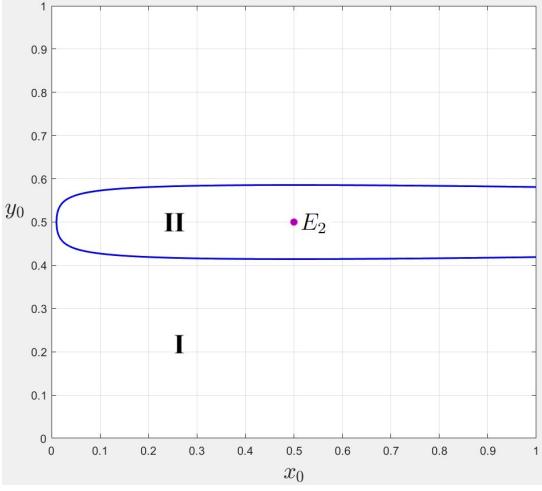
Figure 7: The graph of the curve (29), when η = 2, ε = 0,01, K = 1.
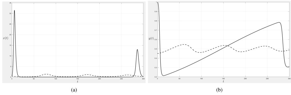
Figure 8: Fast-slow structure on the population of (a) predator and (b) prey.
6. CONCLUSION
We have investigated the behavior of the predator-prey model with carrying capacity. The model exhibits two saddle-type equilibria and one stable spiral equilibrium. Specifically, solution trajectories converge to the unique equilibrium point \((E_2)\) in the first quadrant.
Using GSPT, the model is divided into two subsystems: the slow flow given by \(\dot{y} = y(1-x-y)\) and the fast flow dependent on the critical manifold \(C_0\) when \(\varepsilon = 0\). The critical manifold is attracting for \(0 < y < \frac{1}{\eta}\), repelling for \(y > \frac{1}{n}\), and loses its hyperbolic normality at \(y = \frac{1}{n}\).
repelling for \(y>\frac{1}{\eta}\), and loses its hyperbolic normality at \(y=\frac{1}{\eta}\). Specifically, the solution behavior from the slow subsystem to the fast subsystem is analyzed, finding functions F and G. It has been demonstrated that these solutions converge to the equilibrium point \(E_2\). In conclusion, this research shows that GSPT can be used to analyze and understand the predator-prey model with carrying capacity on prey. Initial conditions have been identified where the predator-prey model with carrying capacity on prey exhibits a fast-slow structure.
ACKNOWLEDGEMENT
R.R. gratefully acknowledges financial support from Directorate of Research and Development, Universitas Indonesia under Hibah PUTI 2023 Grant No. NKB-486/UN2.RST/HKP.05.00/2023.