

1. INTRODUCTION
In the world, a sudden unexpected increase in the number of infected humans with an infectious disease can be experienced at any time. According to the Centers for Disease Control and Prevention, such an increment in the number of infected humans, which occurs in a specific geographical area is considered as an epidemic [1]. From the Plague of Athens during 430 - 426 B.C.E to COVID-19 since 2019, human society has been replete with various kinds of epidemics such as the Black Death, Cholera, Russian Flu, MERS, etc [2], [3]. Those occurrences of epidemics make people motivated continuously to study epidemics.
An epidemic occurs in a sudden disease outbreak. A large number of people in a particular population, region, or community, is affected by an epidemic [4]. Epidemic modeling plays a significant role in providing insight into the transmission dynamics of communicable diseases [5], [6], [7]. The spread of those diseases through a community can be described from such epidemic models [8]. Those models consist of a set of equations that translate the assumptions into a mathematical representation [9].
Human dispersal behaviors play a major role in infectious disease spread. Due to globalization and transportation development, an increase in human dispersal behavior can be observed. Due to the increment of human dispersal behaviors, the transmission speed of infectious diseases got faster [10].
The classical compartmental models are not feasible for incorporating the disease spread with spatial interactions [11]. A more accurate model can be obtained by concentrating on spatially distributed subpopulations [12]. Since the gravity model which is based on Newton's gravitational laws is a spatial interaction model, it is motivated to consider a multi-patch model with the gravity model approach incorporating a compartmental model [13]. The classical epidemic models are mostly based on the assumption that the entire population is well-mixed, and they live in one area. But usually, humans live in different areas and the disease spread is affected by spatial heterogeneity [14]. In epidemiology, such areas are called patches. Metapopulations occur if those patches are connected through human dispersal behaviors [2]. Human dispersal behaviors play a major role in the COVID-19 spread as it is an infectious disease [15].
*Corresponding author
Received May 1st, 2024, Revised October 20th, 2024, Accepted for publication December 11th, 2024. Copyright ©2024 Published by Indonesian Biomathematical Society, e-ISSN: 2549-2896, DOI:10.5614/cbms.2024.7.2.5
In the early stages of COVID-19, traveling restrictions and lockdowns were some of the pivotal nonpharmaceutical interventions (NPIs) used to limit human dispersal behaviors and NPIs dropped off the speed of the spread [16]. Several studies have been conducted to model epidemics with human dispersal behaviors. A study that is focused on understanding the impact of mobility on COVID-19 spread presents the relationship between the spatial interactions and the distance between patches. The spatial interaction is inversely proportional to the distance [16].
According to Newton's law of gravity, the gravitational force between two masses is directly proportional to the product of the two masses and it is inversely proportional to the square of the distance between them. The typical gravity model is based on the Newton's law of gravity. It can be written as:
\[F = \frac{Gm_1m_2}{r^2},\tag{1}\]
where F is the gravitational force, m1 and m2 are the masses of two objects, r is the distance between them and G is a constant [17]. Steward, who was a Princeton astronomer, noticed that Newton's law of gravity is resembled by the spatial interactions. Then the gravity law is incorporated with the spatial interactions by Steward during 1940s. He expressed it as:
\[F = \frac{GP_iP_j}{d_{ij}^2},\tag{2}\]
where F is the demographic force, Pi and Pj are the populations of the origin and the destination respectively, dij is the distance between them and G is a constant [18].
Various forms of gravity models inspired by Newton's law of gravity are widely used in different areas which are incorporated with the spatial interactions. The gravity model has been used in the area of international trade, traffic flows, and human mobility [19], [20]. In 1962, Tinbergen introduced the gravity model concepts into international trade [21]. The gravity model was used for migration flows by Ravenstein in 1889 [22].
The gravity model is developed for human dispersal behaviors. It says that the demographic force is directly proportional to the size of the populations in the patches and inversely proportional to the distance between them [18]. Then the gravity model is written as follows:
\[F_{ij} = K \frac{P_i^n P_j^m}{d_{ij}^{\gamma}}. (3)\]
Since the gravity model is adapted in various domains, generally it can be written as:
\[F_{ij} = K P_i^{\ n} P_j^{\ m} f_\gamma(d_{ij}). \tag{4}\]
With the various studies which have been conducted, the form of a gravity model for the human dispersal behaviors has been generalized and modified. It is influenced by a form of distance decay function (fγ(dij )) where the spatial and social interactions increase as the distance between two locations i and j (dij ) decreases [16]. The distance decay function can be a power law-based function or an exponential law-based function. However, it depends on the distance between the two locations [23].
Table 1: The description of the gravity model used for calculating human dispersal behaviors.
| Symbol | Description |
|---|---|
| Fij | th patch to th patch Number of people moving from i j |
| Pi, Pj | th and th patches Population in i j |
| dij | Geographical distance between patch i and j |
| K | Proportionality constant |
| n, m, γ | Parameters to be estimated |
| N | Number of patches. |
To model a compartmental model with a gravity model approach, creating a mobility matrix is a major concern. If someone uses the gravity model for human dispersal behaviors within a patch, Fij becomes undefined because the distance from a patch to the same patch dij is zero. There was a lot of literature that tried to overcome that problem. In literature, the gravity model was used to find the number of trips between two geographical locations. The probability of mobility within a patch was explained with weighted average methods [24]. In some literature, the volume of interactions (contacts) between patches is given by a gravity model approach. There they used the typical gravity equation in Equation 2 for modeling the contacts between two patches. The radius of a circle with an area equal to the area of the patch is used to \(d_{ij}\) instead of the distance to model the contacts within the patch [12].
The researchers are interested in using a gravity model approach to model an epidemic in a patchy environment. A study on a two-patch system brings out the gravity model to model the rate of change of the number of humans in a particular patch. That does not model human mobility within a patch [25]. The rate of mobility within and between patches is modeled separately in previous incidences. Therefore, it is interesting to look for a method that can incorporate the rate of human dispersal behaviors within and between patches in the same gravity model approach. The gravity model is used as a model to measure human dispersal behaviors. In a study on the influenza epidemic in the United States of America, the major aspects of workflows are apprehended using a piece-wise gravity model [26].
The infectious diseases are classified as human-to-human transmitted diseases, food and waterborne diseases, and vector-borne diseases [2]. Since the study is directed to a gravity model approach with human dispersal behavior, the study is focused on human-to-human transmitted diseases. The recent infectious disease; COVID-19 which later became a global epidemic is a viral infectious disease that emerged in Wuhan City, Hubei province, China in December 2019 [27]. It was caused by Severe Acute Respiratory Syndrome Coronavirus 2 (SARS-CoV-2). It transmits from human to human by direct contact and droplets. It was spread all over the world with a 2% - 3% fatality rate [28], and resulted in 775,132,086 cases including 7,042,222 deaths globally [29]. Including Sri Langka, 229 countries and territories were burdened by COVID-19. In Sri Lanka, the first patient found on the \(27^{th}\) of January 2020 was a Chinese woman, and the first confirmed local case was reported on the \(11^{th}\) of March 2020 in Sri Lanka [30]. Then the whole population was susceptible and 672 754 confirmed cases with 16 889 deaths were reported [31].
Sri Lanka is divided into 9 provinces for administrative purposes which are named Western, Southern, Central, North Western, North Central, Uva, Sabaragamuwa, Northern, and Eastern. Human dispersal behaviors spread through those provinces due to educational purposes, career purposes, freight transportation, and various other reasons.
In Sri Lanka, the gravity model approach is used to study the apparel exports, exports, trade, and decision support areas [32], [33]. There is room to research about the transmission of COVID-19 from a Sri Lankan perspective by a gravity model approach with human dispersal behaviors. To address these gaps, a gravity model approach to model human-to-human transmitted epidemic with human dispersal behaviors with a specific focus on studying the spread of COVID-19 within and between different provinces with human dispersal behaviors in Sri Lanka can be started.
The main objective of this research is to formulate a multi-patch epidemic model via a gravity model approach by identifying a way to model human dispersal behaviors within a patch using the gravity model. It incorporates the probability matrix of human dispersal behaviors by using the gravity model concept to investigate the transmission patterns of an epidemic numerically with human dispersal behaviors.
2. MODEL FORMULATION
2.1. Modified gravity model
The gravity model discussed in Equation 4 is used to create the mobility matrix for human dispersal behaviors. Since the generalized gravity model discussed in Equation 3 can not express the mobility within a patch, a need to find a way to express the mobility within a patch is raised. The distance from a patch to the same patch is zero. The mobility will be undefined if the gravity model in Equation 3 is used. Because a division of zero occurs then. Hence, a suitable function for the distance decay function \((f_{\gamma}(d_{ij}))\) mentioned in Equation 4 must be chosen.
The gravity models can be studied in two ways concerning the type of distance decay functions. The power-based gravity model and the exponential-based gravity models are the two types. In the power-based gravity model, an inverse power function is used as the distance decay function. A negative exponential function is used as the distance decay function for the exponential-based gravity model. In Newton's gravity model, the distance decay function is an inverse power function.
An action at a distance that properly reflects the spatial interaction nature is suggested by the inverse power function. But a reflection of spatial interactions between distant patches can not be gained by the negative exponential function [34].
There are two laws of Geography stated as follows by Waldo R. Tobler and G. Arbia.
- 1) "Everything is related to everything else, but near things are more related than distant things [35]."
- 2) "Everything is related to everything else, but things observed at a coarse spatial resolution are more related than things observed at a finer resolution [36]."
These laws are based on the typical gravity model and action at a distance. The inverse proportional property of the distance and the direct proportional property of the sizes of populations are reflected by the above laws respectively. But the negative exponential distance decay function refuses it. Also power based gravity model can express complex networks. Hence, choosing the inverse power function as the distance decay function is more appropriate than choosing the negative exponential distance decay function [34].
In a study for understanding the impact of human dispersal behaviors on the spread of infectious disease, the human dispersal behaviors within and between patches are captured based on the relationship between distance. A model is presented as an inverse power distance decay function by considering that relationship as,
\[f_{\gamma}(d_{ij}) = \frac{1}{(1+d_{ij})^{\gamma}},\tag{5}\] where dij is the distance between patch i and j and γ is a parameter to be estimated [16]. This solves the problematic scenario of division by zero that occurs in the gravity model discussed in Equation 3. Hence, the modified gravity model can be written as follows:
\[F_{ij} = K \frac{P_i^{\ n} P_j^{\ m}}{(1 + d_{ij})^{\gamma}}.\] (6)
All the symbols that are used in Equation 6 are described in Table 1.
2.2. Parameter estimation
1) Using OLS method: The typical gravity model explained in Equation 1, has its' population exponents as 1 and the distance exponent as 2. But in the context of epidemiology, the gravity model concept is used to capture the human dispersal behaviors. According to many studies, the exponents in the modified gravity model in Equation 6 rarely be the same as the typical gravity model in Equation 1 [23], [25], [26]. Hence, a parameter estimation must be executed to find the appropriate values for the parameters n, m, γ, and K in the modified gravity model (Equation 6).
The most common way to estimate the gravity parameters is the ordinary least squares (OLS) method. To perform the OLS estimation, the modified gravity model equation must be log-linearised as follows:
\[\ln F_{ij} = \ln K + n \ln P_i + m \ln P_j - \gamma \ln (1 + d_{ij}). \tag{7}\]
Then the mobility data, population data, and the distances related to the nine provinces in Sri Lanka are used to fit the log-linearised model in Equation 7. The built-in function 'minimize' in scipy.optimize in SciPy python library, is used to minimize the sum of squares of the residual sum. Here initial guesses for the parameters n, m, γ and K must be provided to complete the procedure.
2) Initial guesses: The initial guesses for n, m, and γ are guessed from literature. A study of disease spread with a piecewise gravity model that incorporates workflows gives two sets of values for n, m, and γ such as (0.30, 0.64, 3.05) and (0.24, 0.14, 0.29) [26]. Also, γ is found to be in the range of (0.5 − 3.0) in various studies for different data sets [20]. Hence, the initial guesses are chosen as n = 0.27, m = 0.39, and γ = 1.67.
To make an initial guess for the proportionality constant K, the following steps that are widely used in the area of physics are taken into consideration. First, the modified gravity model in Equation 6 must be written in the form of y = m0x where Fij acts as the dependent variable (y) and Pi nPj m (1 + dij ) γ acts as the independent variable (x). Then the K starts to work as the slope (m0).
\[\underbrace{F_{ij}}_{y} = \underbrace{K}_{m_0} \underbrace{\frac{P_i^n P_j^m}{(1 + d_{ij})^{\gamma}}}_{x} \tag{8}\]
Here the parameter values used in sub-section 2.2.2 are used to evaluate the x values in Equation 8. To find the value of K, a polynomial with degree 1 which is a line is fitted to the data. The built-in function 'polyfit()' in Python NumPy library is used to do that task. Then ln K is given as the initial guess to the OLS method where ln K = 4.83. Therefore, (0.27, 0.39, 1.67, 4.83) are given as the initial guesses for (n, m, γ, ln K) in OLS method.
- 3) Using NLS method: The OLS method for a log linearised model has some drawbacks in estimating parameters. It can not perform parameter estimation if the dependent variable of the model becomes zero. In the context of our study, parameter estimation could not be done by OLS if there is zero mobility from patch i to patch j.(i.e. Fij = 0). Because when we log-linearise the model, then ln Fij becomes undefined as ln 0 has not been defined. This problem is not encountered with the nonlinear least squares (NLS) method. Also, it can estimate parameters without log linearising the model. The built-in function 'least_squares' in scipy.optimize in SciPy python library, is used to minimize the sum of squares of the residual sum. Here also initial guesses for the parameters n, m, γ, and K must be provided to complete the procedure.
- 4) Using the Hybrid OLS-NLS method: The NLS method is sensitive to the initial guesses. Therefore, it is important to have proper initial guesses for the parameter values to be estimated before using the NLS method.
Considering all aspects, the hybrid OLS-NLS method is introduced to estimate parameters by combining OLS and NLS methods. The steps are discussed below.
- 1) Choose appropriate initial guesses for the parameters to be estimated as discussed in sub-section 2.2.2.
- 2) Log linearise the modified gravity model as Equation 6.
- 3) Estimate parameters using the OLS with above mentioned initial guesses.
- 4) Use the estimated parameters from the OLS, as the initial guesses for the NLS method.
- 5) Estimate the parameters using the NLS method.
The estimated parameters will be discussed in Section 3.1
2.3. Mobility matrix
In this stage, the parameters in the modified gravity model 6 have been estimated as relevant to the mobility data of the provinces in Sri Lanka. The gravity model gives the number of people traveling from patch i to patch j. The mobility rate from patch i to j is denoted as pij . It is calculated by considering the proportion of patch i humans who are traveling in patch j. And it gives the probability of moving a human from patch i to patch j. Also, the mobility matrix which is the probability matrix of human dispersal behaviors can be denoted as,
\[\pi = (\pi_{ij})_{9 \times 9}, \quad i, j = 1, 2, ..., 9,\] (9)
where i and j are the provinces.
Then the mobility rate from province i to j can be determined by,
\[\pi_{ij} = \frac{F_{ij}}{9}, \qquad (10)\] \[\sum_{j=1}^{9} F_{ij}\]
where i, j = 1, 2, ..., 9. Therefore,X 9 j=1 πij = 1. Also the diagonal entries of the mobility matrix (πii), ∀i ∈ {1, 2, ..., 9}
provide the probability of moving a human from his residence patch to the same. The calculated mobility matrix which gives the probability matrix of human dispersal behaviors within and between the 9 provinces in Sri Lanka will be discussed in the Section 3.1.
2.4. Residence budgeting time matrix
The residence budgeting time matrix for the nine provinces in Sri Lanka is linked with the mobility matrix for nine provinces which is given in Equation 9. Most humans in Sri Lanka make short-term movements within and between provinces because of education and career purposes. Generally, Sri Lankan people have 8 working hours and we assume that it takes 2 hours to travel from home to the workplace and back to home. Therefore, we assume the proportion of time that a human travels from province i to other provinces \((t_i)\) is \(\frac{10}{24}\) Then,
\[P = \frac{14}{24}I_9 + \frac{10}{24}\pi,\tag{11}\]
where \[\pi = (\pi_{ij})_{9\times 9}\], \(P = (p_{ij})_{9\times 9}\), and \(I_9\) is the identity matrix of size 9. Also, \(\sum_{j=1}^{9} \pi_{ij} = \sum_{j=1}^{9} p_{ij} = 1\), \(\forall i \in \{1, 2, ..., 9\}\).
2.5. Multi-patch SIR model with human dispersal behaviors
The classical SIR model is formulated on a well-mixed population that lives in the same area. However, in real-world scenarios, the spatial heterogeneity must be included in the model. The spatial interactions and the connection between different populations in patches occur with the human dispersal behaviors [2]. The movements of individuals that are caused by human dispersal behaviors can be classified as short-term movements and long-term movements.
When humans spend more time in their residence patch and visit another patch or patches to spend less time in that patch, such a movement is called a short-term movement. They come back to their residence patch after spending a certain proportion of time in another patch. Humans settle in another patch which is not their residence patch and those movements are called long-term movements. The modeling approaches are different concerning the type of dispersal behavior. The Lagrangian approach which is related to fluid dynamics is used when it comes to short-term movements and it becomes the Eularien approach with long-term movements [37]. The study highlights the Lagrangian approach.
First, we assume that the total population consists of N number of patches that are connected with human dispersal behaviors. Those patches can be geographical locations or any groups of people. We assumed that any individual in a patch visits another patch to spend some time and return to the residence patch. An individual can infect another individual in his residence patch or any other patch. Also, a healthy individual can be infected at his residence patch or any other patch [2].
In each patch, there are three compartments which are susceptible, infected, and recovered classes. The summation of those three compartments gives the total number of humans in a patch. \(N_i = S_i + I_i + R_i\).
The total population \[N_{total}\] is given by, \(N_{total} = \sum_{i=1}^{N} N_i\).
Table 2: The description of the symbols used in multi-patch SIR model.
| Symbol | Description |
|---|---|
| \(\overline{S_i}\) | The number of susceptible individuals in patch \(i\) |
| \(I_i\) | The number of infected individuals in patch \(i\) |
| \(R_i\) | The number of recovered individuals in patch \(i\) |
| \(N_i\) | The total population in patch \(i\) |
| N | Number of patches |
| \(p_{ij}\) | The proportion of time that humans in patch \(i\) move in patch \(j\) |
| \(\beta_j\) | Transmission rate in patch \(i\) |
| \(\alpha_i\) | Recovery rate in patch i |
The multi-patch (meta-population) model represents its model in a large system of ordinary differential equations [2]. The ODE system can be written as follows [38]:
\[\frac{dS_i}{dt} = -S_i \sum_{j=1}^N \beta_j p_{ij} \left( \frac{\sum_{k=1}^N p_{kj} I_k}{\sum_{k=1}^N p_{kj} N_k} \right), \qquad S_i(t_0) \ge 0,\] \[\frac{dI_i}{dt} = S_i \sum_{j=1}^N \beta_j p_{ij} \left( \frac{\sum_{k=1}^N p_{kj} I_k}{\sum_{k=1}^N p_{kj} N_k} \right) - \alpha_i I_i, \quad I_i(t_0) \ge 0,\] \[\frac{dR_i}{dt} = \alpha_i I_i, \qquad R_i(t_0) \ge 0,\] (12)
where \[i, j, k = 1, 2, ..., N\] and \(\sum_{i=1}^{N} p_{ij} = 1\).
j=1 In Sri Lanka, there are nine distinct provinces for administrative purposes [39]. They can be considered as patches that are connected with human dispersal behaviors. A type of multi-patch compartmental model discussed in the Equation 12, which is a nine-patch SIR model is used to investigate the COVID-19 spread within and between Sri Lanka. The results calculated by the residence budgeting time matrix are used for the pij values in Equation 12.
The transmission rate βj , captures the risk of infection in patch j. And the infection rate of the patch i is,
\[\sum_{j=1}^{9} \beta_j p_{ij} \left( \frac{\sum_{k=1}^{9} p_{kj} I_k}{\sum_{k=1}^{9} p_{kj} N_k} \right).\]
Here the number of newly infected humans belonging to patch i who got infected while moving within their residence patch i is given by,
\[S_i \beta_i p_{ii} \left( \frac{\sum_{k=1}^9 p_{ki} I_k}{\sum_{k=1}^9 p_{ki} N_k} \right).\]
The number of new infected humans belongs to patch i who got infected while moving between their residence patch i and the other patches j is given by,
\[S_{i} \sum_{j=1, j \neq i}^{9} \beta_{j} p_{ij} \left( \frac{\sum_{k=1}^{9} p_{kj} I_{k}}{\sum_{k=1}^{9} p_{kj} N_{k}} \right).\]
Also, the proportion of time that residents from patch j spend in patch j is denoted by pjj and pij denotes the proportion of time that residents from patch i spend in patch j.
Here all the infected humans are assumed to be infectious and all the recovered humans are assumed not to be susceptible again. Since the time duration of the disease is negligible compared to the lifetime of a human, the total population in the country is assumed to be constant.
2.6. Basic reproduction number \((\mathcal{R}_0)\)
The next generation matrix method which is introduced by Diekmann, is widely used to derive the reproduction number for models that incorporate the spatial structures [40]. The next generation matrix G is created as, \(G = FV^{-1}\), where F and V are the jacobians of the new infections appearance rate in the \(i^{th}\) compartment \((\mathcal{F}_i(\vec{\mathbf{x}}))\) and the difference of the transfer rate of individuals into the compartment i and out of the compartment i (\(\mathcal{V}_i(\vec{\mathbf{x}})\)) at the disease free equilibrium point.
\[F = \frac{\partial \mathcal{F}_i(x_0)}{\partial x_i}\] and \(V = \frac{\partial \mathcal{V}_i(x_0)}{\partial x_i}\).
Here the vector \(\vec{\mathbf{x}}\) is denoted as, \(\vec{\mathbf{x}} = x_i, i = 1, 2, ..., q\) where q is the number of compartments in the system and \(x_i\) is the size of the \(i^{th}\) compartment or the proportion of individuals in the \(i^{th}\) compartment. Then the dominant eigenvalue of matrix G which is the spectral radius of G is defined as the reproduction number \((\mathcal{R}_0)\) [41].
3. Numerical Results
3.1. Parameter estimation of the gravity model
The parameter estimation for the modified gravity model in Equation 6 is performed using OLS, NLS, and hybrid OLS-NLS methods as discussed in Section 2.2. The values described in sub-section 2.2.2 are given as the initial guesses for the estimation. The following are the estimated values for the gravity model parameters relevant to each estimation method.
Table 3: The estimated parameter values for the gravity model using OLS, NLS, and hybrid OLS-NLS methods,
| OLS method | NLS method | Hybrid OLS-NLS method | |
|---|---|---|---|
| \(\overline{n}\) | 0.69994 | 0.27105 | 0.38326 |
| m | 0.94025 | 0.39114 | 0.60072 |
| \(\gamma\) | 0.83117 | 1.66548 | 0.77417 |
| K | 1.00007 | 124.72659 | 1.00977 |
From the three types of above estimation methods, three sets of parameters are obtained as the gravity model parameters. The following set of parameters which is obtained by the hybrid OLS-NLS method, is used as the parameters of the modified gravity model in Equation 6 in this research. The reason behind choosing this set of parameters is discussed in Section 4 considering the model evaluation metrics.
\[n = 0.38326, \quad m = 0.60072, \quad \gamma = 0.77417, \quad K = 1.00977\] (13)
3.2. The mobility matrix
The gravity model approach is used to create the mobility matrix by following the method discussed in Section 2.3. The distances between the nine provinces, populations in the nine provinces, and the parameter values estimated in Equations 13 are provided to the modified gravity model in Equation 6. Then the mobility matrix \(\pi\) is created as the above Figure 1. It shows that the probability within a province takes a higher value than between provinces.
Generally, the mobility within a patch takes a higher value than between the patches. That aspect is also captured by this gravity model approach and represented in diagonal values \((\pi_{ii}), \forall i \in \{1, 2, ..., 9\}\) of the mobility matrix \(\pi\).
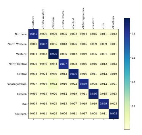
Figure 1: The mobility matrix for nine provinces in Sri Lanka obtained by the gravity model approach.
3.3. Visualization of the probabilities between provinces
Here we visualize the pattern of mobility between provinces. Mobility within a province is not included here.
1) Visualization with distances: Figure 2 shows how the human dispersal behaviors between provinces behave concerning the distance between the provinces. The values of the x-axis of each plot in Figure 2 are sorted in ascending order concerning the distance from each province to the other provinces.
The probabilities of human dispersal behaviors are almost reduced with the increment of the distance between provinces according to Figure 2. However, an increment is observed in the Western province in each plot though some other provinces have higher distances than the Western Province. According to the Equation 6, the populations of the provinces and the distance between them affect the human dispersal behaviors. The Western province has the highest population and it is the reason for the above-mentioned observation.
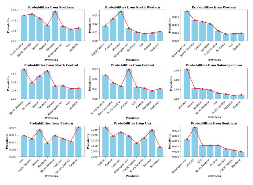
Figure 2: Human dispersal behaviors with the distances between provinces in each province in Sri Lanka.
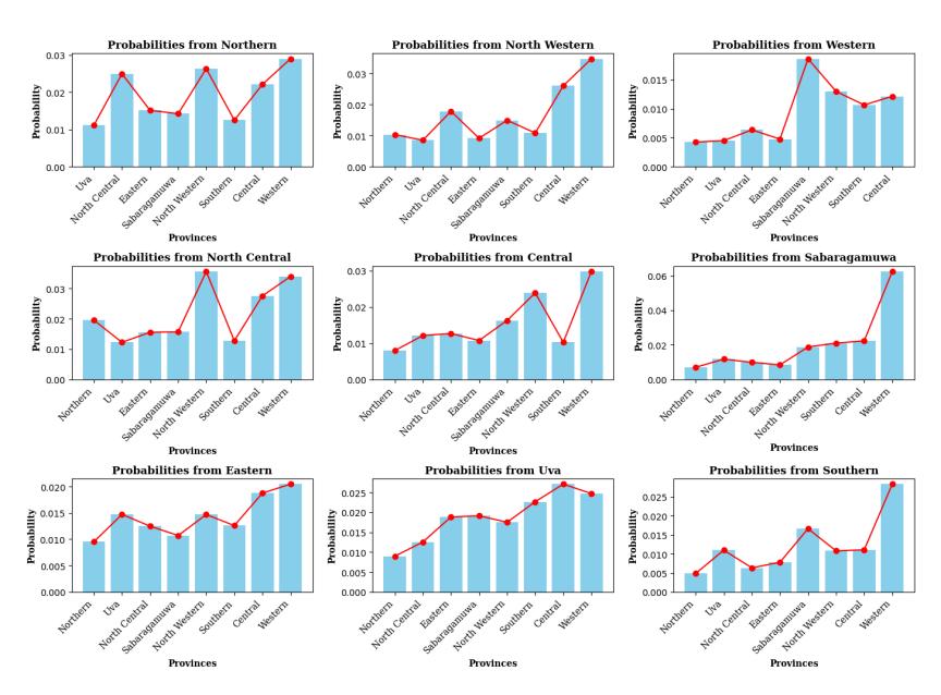
Figure 3: Human dispersal behaviors between provinces with the population size of the destination province in each province in Sri Lanka.
- 2) Visualization with population: The behavior of the human dispersal behaviors between provinces concerning the population of the destination province for each province is shown in Figure 3. The x-axis values of each plot in Figure 3 are sorted in ascending order concerning the population of the destination province. The probabilities of human dispersal behaviors are increasing when the population of the destination province is high. But it is changed due to the effect from distance as discussed through the modified gravity model in Equation 6.
- 3) Visualization with distance and population: The effects of both distance and population on the probability and the human dispersal behavior between provinces are presented in Figure 4. It represents the relationship between the probability of human dispersal behaviors between provinces with the population of the destination province and the distances between provinces in each province in Sri Lanka. The values of the x-axis and the values of the y-axis are sorted in ascending order concerning the distance between the provinces and the population of the destination province respectively.
3.4. The residence budgeting time matrix
Assuming that a human in i th province spends 10 hours in any other province, the residence budgeting time matrix can be obtained using Equation 11.
3.5. Parameter estimation of multi-patch SIR model
The multi-patch SIR model in Equation 12, is used to incorporate the human dispersal behaviors into the COVID-19 disease spread. The calculated number of infectious humans using Equation 12 and the real data for infectious humans are considered to estimate the transmission rates for each province in Sri Lanka as shown in Table 4.
1) Fixed parameters: Sri Lanka is a small island with a small crowd of population compared to some other big countries like India, the USA, Russia, etc. Therefore, the recovery rates (αi) of the humans in province i for all nine provinces are assumed to be the same α. Therefore, the recovery rate α for all provinces in Sri Lanka is considered as a fixed parameter such that α −1 = 10.25 days [42].
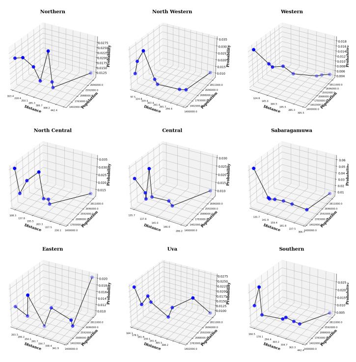
Figure 4: Human dispersal behaviors with the population of the destination province and the distances between provinces.
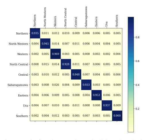
Figure 5: The residence budgeting time matrix for nine provinces in Sri Lanka obtained by the gravity model approach.
2) Estimated parameters: The estimated parameter values for the βi for each province are shown in the Table 4. Neither lockdown nor social distancing strategies are considered in the estimation. Those estimations are done as the methods discussed in follows.
The built-in function 'least_squares' in scipy.optimize in SciPy python library, is used to estimate the βi values. The non-linear least squares method is used to minimize the sum of squares of the residual sum. The residuals are the difference between the actual data and the predicted data from the relevant ODE system.
The data on the number of infected and susceptible humans, populations in each province, and the residence budgeting time matrix time obtained in 5 by the gravity model approach is used in the estimating process. Also, the recovery rates for each province \((\alpha_i)\) are considered to have the same value \(\alpha\). For this research, Northern, North Western, Western, North Central, Central, Sabaraganuwa, Eastern, Uva, and Southern provinces are indexed as 1, 2, 3, 4, 5, 6, 7, 8, and 9 respectively.
| Symbol | Related Province | Value |
| \(\beta_1\) | Northern province | 0.07344980 |
| \(\beta_2\) | North Western province | 0.13890953 |
| \(\beta_3\) | Western province | 0.12895880 |
| \(\beta_4\) | North Central province | 0.02554977 |
| \(\beta_5\) | Central province | 0.11607572 |
| \(\beta_6\) | Sabaragamuwa province | 0.00473791 |
| \(\beta_7\) | Eastern province | 0.00972736 |
| \(\beta_8\) | Uva province | 0.00020758 |
| \(\beta_9\) | Southern province | 0.11356019 |
Table 4: Estimated values for the transmission rates \((\beta_i)\) of each province.
3.6. Impact of human dispersal behaviors into disease spread
The human dispersal behaviors were restricted by imposing lockdowns to decrease the COVID-19 spread in Sri Lanka. Hence a lockdown variable; \(L_i\) is introduced to demonstrate the impact of human dispersal behaviors on disease spread. The lockdown strength of \(i^{th}\) province is given by \(L_i\) which takes the values between 0 and 1. When the lockdown strength becomes 1, it denotes no human dispersal behaviors [43]. According to the literature, it causes a new transmission rate in province i (\(\tilde{\beta}_i\)) such that, \(\tilde{\beta}_i = (1 - L_i)\beta_i\).
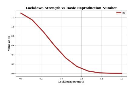
Figure 6: Basic reproduction number for different lockdown strengths.
4. DISCUSSION AND CONCLUSIONS
Epidemic modeling by a gravity model approach is getting more attention and it is becoming interesting to study among the researchers. When it comes to meta-population modeling using compartmental models, the gravity model used in Equation 3, could not be used to model the human dispersal behaviors within a patch. It only models the human dispersal behaviors between patches. Because the denominator of the gravity model Equation 3 becomes zero as explained in Section 2.1, when the human dispersal behaviors within a patch are considered. By modifying the gravity model as the Equation 6, the barriers to model the human dispersal behaviors within a patch disappear.
The human dispersal behaviors within a patch are observed to be greater than the behaviors between the patches in actual mobility data. Choosing the distance decay function \(f_{\gamma}(d_{ij})\) in the gravity model as \(\frac{1}{(1+d_{ij})^{\gamma}}\) instead of \(\frac{1}{(d_{ij})^{\gamma}}\) effectively captures the above-mentioned scenario and it also solves the problem of division by zero discussed in Section 2.1.
The distances between any provinces i and j which is denoted as \(d_{ij}\) is greater than 50km in Sri Lanka. \((d_{ij} > 50 \text{km}, \forall i, j \in \{1, 2, ..., 9\} \text{ where } i \neq j)\). Therefore,
\[\mathbf{f}_{\gamma}(d_{ij}) = \begin{cases} \frac{1}{(1 + d_{ij})^{\gamma}} < \frac{1}{51^{\gamma}}, & \text{if } i = j\\ \frac{1}{(1 + d_{ii})^{\gamma}} = 1, & \text{if } i \neq j \end{cases}\]
\(\forall i \in \{1, 2, ..., 9\} \text{ where } \gamma = 0.77417147.\)
Hence, \(f_{\gamma}(d_{ii}) > f_{\gamma}(d_{ij}), \forall i,j \in \{1,2,...,9\}\) where \(i \neq j\). Therefore, the magnitude of the effect given by the distance decay function related to the human dispersal behaviors within a patch is greater than the magnitude of the effect given by the distance decay function related to the behaviors between patches. That explanation justifies the reason for capturing the higher human dispersal behavior rates within a patch by the modified gravity model in Equation 6. That scenario is represented visually in Figure 1.
The parameters of the modified gravity model in Equation 6 are estimated using three different methods as discussed in Section 3.1. Three different model evaluation metric values are calculated for all those sets of parameters obtained by above mentioned types of estimation methods. The R-squared, RMSE (Root Mean Square Error), and MAE (Mean Average Error) values are calculated for each model that carries different parameter values due to the difference in the estimation method.
Table 5: R-squared, RMSE, and MAE values across different estimation methods.
| OLS method | NLS method | Hybrid OLS-NLS method | |
|---|---|---|---|
| R-squared | 0.8858 | 0.7868 | 0.8963 |
| RMSE | 0.0799 | 0.1091 | 0.0761 |
| MAE | 0.0378 | 0.0546 | 0.0365 |
The lowest R-squared value and the highest RMSE and MAE values can observed in the model that uses the NLS method to estimate parameters. It occurs because of the high sensitivity to the initial guesses. At the same time, the hybrid OLS-NLS method discussed in sub-section 2.2.4, provides the highest value for R-squared and the lowest values for the RMSE and MAE. Therefore, parameter estimation using the hybrid OLS-NLS method gives better parameter values for the gravity model compared to the other two methods. Therefore, in this study, the parameters estimated using the hybrid OLS-NLS method are used as the parameters for the modified gravity model in Equation 6 which are (0.38326244, 0.60072182, 0.77417147, 1.00976875) for \((n, m, \gamma, K)\).
The parameter estimation method used in this research to estimate the gravity model parameters is the hybrid OLS-NLS method that combines the OLS and NLS methods. Since the parameters must be estimated using the OLS method with the log-linearised gravity model, only non-zero mobility included data can be used for the parameter estimation.
The relationship between the dependent variable \(F_{ij}\) and the independent variables \(P_i, P_j\), and \(d_{ij}\) of the modified gravity model in Equation 6, can be displayed using the double-log functional form of the modified gravity model. The double-log functional form of it can be written as:
\[\ln(F_{ij}) = \ln K + n \ln(P_i) + m \ln(P_j) - \gamma \ln(1 + d_{ij}).\]
Then the n, m, and \(\gamma\) are the elasticity coefficients that represent how the dependent variable is affected by a change in independent variables.
It suggests that a 1% increase in the population of the residence province i causes a 0.38326% increase in the number of human movements from province i to province j. Also, it suggests that a result of a 0.60072% increase in the number of human movements from province i to j is caused by a 1% increase in the population of the province j. But a 1% increase in the distance decay function such that, \(f_{\gamma}(d_{ij}) = \frac{1}{(1+d_{ij})^{\gamma}}\) makes a 0.77417% decrease in the number of human movements from province i to j.
Then the mobility rates can be calculated using the equation introduced in Equation 10. Hence,
\[\pi_{ij} = \frac{K \frac{P_i^n P_j^m}{(1 + d_{ij})^{\gamma}}}{\sum_{j=1}^{9} K \frac{P_i^n P_j^m}{(1 + d_{ij})^{\gamma}}}, \quad \forall i \in \{1, 2, ..., 9\}.\]
Therefore, the proportionality constant K can be canceled off in the stage of the mobility rates calculation and it does not affect the mobility rates because,
\[\pi_{ij} = \frac{\frac{P_i^n P_j^m}{(1 + d_{ij})^{\gamma}}}{\sum_{j=1}^{9} \frac{P_i^n P_j^m}{(1 + d_{ij})^{\gamma}}}, \quad \forall i \in \{1, 2, ..., 9\}.\]
In Sri Lanka, there is a lack of mobility data. Only the data on buses are available as the mobility data. But there are many other traveling modes commonly used in Sri Lanka. Therefore, the parameter estimation for the gravity model is done with a limited number of mobility data.
The variation of the basic reproduction number with the lockdown strength can be observed in Figure 6. It shows that the reproduction number will be reduced when the lockdown strength of all provinces become increased which provides the decrease of the human dispersal behaviors. Therefore, the reduction of human dispersal behaviors causes to the reduction of the basic reproduction number. The disease die out when the human dispersal behavior become reduced to 80% because R0 < 1 when the lockdown strength is 0.2.
In the initial stages of infectious disease, it is not practical to impose a full lockdown for a long time. Because it may cause various social and economic problems. Therefore the country is clustered into 3 clusters
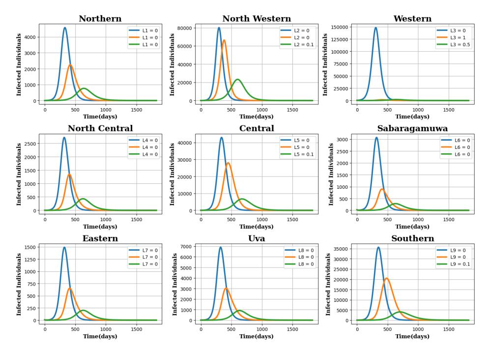
Figure 7: The infected human population over time in no lockdown, high zone lockdown, and high and moderate zone lockdown.
namely high-risk zone, moderate-risk zone and low-risk zone based on the number of infected humans in each province at their peak. The clustering is done using the K-Mean clustering.
Table 6: Clusters.
| Zone | Provinces |
|---|---|
| High-risk | Western |
| Moderate-risk | Southern, North Western, Central |
| Low-risk | Other provinces |
This clustering provides the opportunity to impose separate lockdowns with different strengths into separate clusters. Figure 7 shows infected curves for different lockdown scenarios for each province.
The infected curves when there is no lockdown are shown in blue colored curves and the orange color curves represent the infected curves when there is a full lockdown in the high-risk zone. The green-colored curves provide the infected curves when there are lockdowns with 0.5 and 0.1 lockdown strengths in highrisk zone and moderate-risk zone respectively. The least peaks for each province are provided by the last lockdown scenario.
5. FUTURE WORK
Since the gravity model gives an effective insight into modeling the patterns of human dispersal behaviors, this research can be extended to model the effects of the lockdown on the human dispersal behaviors and the patterns of human mobility amidst a lockdown incorporating the gravity model.
A transformation of the mobility matrix in Figure 1 into another mobility matrix which indicates the lockdown effects on the mobility within and between the provinces will be a new approach to model the lockdown effects on human dispersal behaviors. The transformation can be considered to be done using another matrix and multiplying it with the existing mobility matrix. Finding such a matrix that incorporates the lockdown measures will be an extension of this research.
In this research, a multi-patch SIR model with three compartments: susceptible, infected, and recovered are used. We can extend the multi-patch SIR model by incorporating another compartment or compartments such as dead, quarantined, and vaccinated compartments. It would be a more realistic capture of the realworld scenario of COVID-19 transmission. It will also open the research to a path of an extended version of epidemic modeling research incorporated with optimal control problems.
6. DATA AVAILABILITY
The population data for each province is taken from the Registrar General's Department of Sri Lanka [44]. The distances between the provinces are taken as mentioned in the Road Development Authority [45]. The mobility data is provided by the National Transport Commission of Sri Lanka. The COVID-19 situation reports from 15th of November 2020 to 10th of December 2020 are used as the data for number of COVID-19 patients [46].