

1. INTRODUCTION
In democratic countries, one of the fundamental pillars of modern democracy is political participation. The citizen's significance in political decision-making is underscored by the electoral process. A decision-making process called an election is used to choose someone for a formal office. Democracy typically employs this mechanism to appoint officials in the legislature and parliament. The act of abstaining from elections, regarded as a simple means of withdrawing from political decision-making, has been found to be prevalent among individuals from diverse social backgrounds. Voters might find renewed motivation to engage if a political alternative is provided that acknowledges and supports their capabilities. The interest of a political party is piqued by the unutilized backing of the marginalized, as the party's platform resonates with disillusioned voters through its straightforward messages and less complex organizational framework [1], [2]. These things can be realized through educational campaigns and argumentative schemes [4], [5]. This might be an attempt to manipulate voters [7]. An educational campaign aims to promote voter turnout in democratic elections by reaching the public through various platforms. Beyond that, argumentation schemes can improve overall voter participation elections. Through debates, candidates use argumentation schemes to present their backgrounds, visions, and missions. The dynamics of voter behavior are very interesting to study mathematically.
Generally, the behavioral stages in the any problem studied by researches. By utilizing mathematical modeling, the various problems are successfully resolved. For examples: crime case [11], [12], the application of pesticides to control plant disease [16], case of COVID-19 in Wuhan [15], case of COVID-19 in Spain and Italy [19], case of COVID-19 by factoring in asymptomatic infections and the effectiveness of health
*Corresponding author
Received June 21st, 2024, Revised October 18th, 2024 (first), Revised December 20th, 2024 (second), Accepted for publication December 23rd, 2024. Copyright ©2024 Published by Indonesian Biomathematical Society, e-ISSN: 2549-2896, DOI:10.5614/cbms.2024.7.2.4
policies and protocols [18], case of dengue transmission [17], [20], the effects of saturated incidence and incomplete treatment in the disease transmission [21], case of measles disease [22], case of HIV/AIDS [23], alcoholism case [13], [14], control of e-rumor [10], behavior of smoking in the society [8], and propagation of computer virus [25]. Regarding elections in democracy, mathematical models have been applied to study voter behavior [4], [5]. The use of mathematical models is vital in determining voter behavior and planning intervention strategies in elections. Additionally, mathematical models offer a robust approach for examining voter behavior in a more accurate manner [6], [3]. Even, discrete time on voting behavior has been studied by Rachik et al. [9]. Despite the emphasis on awareness campaigns [28], [30], the debate is another noteworthy factor to be included in the election model. Measurable notions and ideas become a new challenge to influence voter behavior [29]. Debates provide a platform for election candidates to talk about the issues that matter to the general public. It pertains to how they communicate to shape voters' beliefs [31], [32].
The future behavior of voters can be predicted and the most effective strategy for controlling voter participation can be evaluated using a mathematical model. Specifically, the abstinence situation can be effectively analyzed using the compartment model. Moreover, the complex dynamics of abstinence behaviour can be comprehended using this powerful mathematical model. Here, we propose a mathematical model for abstinence from voting with awareness campaigns and argumentative scheme. Our model is extended from the electoral system by Balatif et al. [5]. The unique aspect of our work is the inclusion of the aware compartment. The paper is organized as follows. We describe the dynamics of voting citizens and their electoral behavior towards a political party in our mathematical model presented in Section 2. The analysis of positivity and boundedness for solutions system is worked in Section 3, while Section 4 explores the existence of equilibrium points and the basic reproductive number. Sensitivity analysis are given in Section 5. In Section 6, we analyze the stability of both local and global equilibriums. Finally, the numerical simulations are discussed in Section 7, and the paper is concluded in Section 8.
2. MODEL FORMULATION
In this section, a novel model is presented to analyze the abstinence behavior from voting in the context of campaigns and argumentation schemes. This section contain assumptions to construct a mathematical model regarding the qualitative behavior of abstaining process. The population is classified into four categories: unaware potential voters \(P_u \equiv P_u(t)\), aware potential voters \(P_a \equiv P_a(t)\), abstainers \(A \equiv A(t)\), and registered \(R \equiv R(t)\). The derivation of Model (1) relies on the following assumptions.
- The recruitment of individuals into the class of unaware potential voters at a rate \(\Lambda > 0\). It is decreased due to campaign awareness, which unaware potential voters into the class of aware potential voters by rate \(\beta_1 > 0\). Furthermore, potential voters can adopt abstention behavior by effectively interacting with existing abstainers by rate \(\alpha > 0\).
- The aware potential voters is decreased due to register on the electoral lists with rate \(\theta > 0\) and the potential for decreased awareness with rate \(\omega > 0\).
- Due to argumentative scheme, Certain abstainers have reversed their decision to boycott the registration on the electoral lists and are now actively participating in the electoral process, resulting in a registration rate of \(\beta_2 > 0\).
- Naturally, the death rate of individu in each classes is \(\delta > 0\).
In Figure 1, the scheme of abstinece behaviour is visually depicted. The model is defined by the system of nonlinear differential equations in (1).
ons in (1). \[\frac{dP_u}{dt} = \Lambda + \omega P_a - \alpha A P_u - (\beta_1 + \delta) P_u, \\ \frac{dP_a}{dt} = \beta_1 P_u - \omega P_a - (\theta + \delta) P_a, \\ \frac{dA}{dt} = \alpha P_u A - (\beta_2 + \delta) A, \\ \frac{dR}{dt} = \theta P_a + \beta_2 A - \delta R.\] (1)
It is important to mention that System (1) is enhanced with a non-negative initial condition.
\[P_u(0) > 0, P_a \ge 0, A \ge 0, R \ge 0,\] (2)
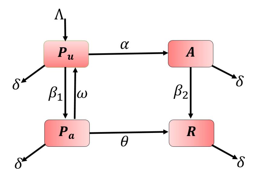
Figure 1: Scheme of abstinence behaviour.
For the sake of convenience, the description and value of parameters in System (1) could be seen in Table 1.
Table 1: Description and value ranges for the parameters in the System (1).
| Parameter | Description | Value | Reference | Units |
|---|---|---|---|---|
| Λ | the recruitment rate of individuals | \(3 \times 10^{6}\) | [5] | People \(\times\) Time-1 |
| \(\alpha\) | the effective contact rate | \(1.2644 \times 10^{-7}\) | Assumed | \((People \times Time)^{-1}\) |
| \(\theta\) | the registration rate of potential voters | 0.04 | [5] | Time-1 |
| \(\omega\) | the unawareness rate of individual | 0.09 | assumed | \(Time^{-1}\) |
| \(\delta\) | the natural death rate | 0.054 | [5] | \(Time^{-1}\) |
| \(\beta_1\) | the registration rate of individuals who were abstainers due to argumentation scheme | 0.5 | Assumed | Time-1 |
| \(\beta_2\) | the awareness rate of individual due to campaign | 0.5 | Assumed | Time-1 |
3. Positivity and Boundedness
This section focuses on investigating the positivity and boundedness of solutions to System (1) when the initial condition is (2).
Theorem 3.1. Any solution \((P_u, P_a, A, R)\) of system (1) with non-negative initial conditions (2) is positive for all time t > 0.
Proof: From System (1), let us consider for A(t) for \(t \ge 0\). Farther in the third equation of System (1), we can get that
\[A(t) = A(0) \exp \int_0^t (\alpha P_u(s) - (\beta_2 + \delta)) ds.\]
From initial conditions in (2), we have A(t) > 0, for \(t \ge 0\). Next, we prove that \(P_u(t), P_a(t)\), and R(t) are positive. Assume the contrary; then, let \(t_1\) be the first time such that \(P_u(t_1) = 0\), \(P_a(t_1) = 0\), and \(R(t_1) = 0\). By the first equation, second equation, and fourth equation of System (1) we have
\[\begin{split} \frac{dP_u}{dt}\Big|_{t=t_1} &= \Lambda + \omega P_a > 0, \\ \frac{dP_a}{dt}\Big|_{t=t_1} &= \beta_1 P_u > 0, \\ \frac{dR}{dt}\Big|_{t=t_1} &= \theta P_a + u_2 A > 0. \end{split}\]
This means \(P_u(t), P_a(t), R(t) < 0\) for \(t \in (t_1 - \varepsilon, t_1)\), where \(\varepsilon\) is an arbitrarily small positive constant. This is contradictory. It follows that \(P_u(t), P_a(t)\), and R(t) are always positive for \(t \ge 0\). This ends the proof.
Theorem 3.2. All solution of System (1) are bounded for all \(t \in [0, t_0]\).
Proof: Since we adding all equation in (1), we get
\[M(t) = P_u(t) + P_a(t) + A(t) + R(t).\] (3)
Next, The derivative of Equation (3) leads to Equation (4).
\[\frac{dM}{dt} = \frac{dP_u}{dt} + \frac{dP_a}{dt} + \frac{dA}{dt} + \frac{dR}{dt}.\] (4)
By substituting System (1) into (3), we get
\[\frac{dM}{dt} = \Lambda - (P_u + P_a + A + R) \delta. \tag{5}\]
For \(M = P_u + P_a + A + R\), we obtain that
\[\frac{dM}{dt} \le \Lambda - M\delta. \tag{6}\]
Thusly,
\[0 \le \lim_{t \to \infty} \sup M(t) \le \frac{\Lambda}{\delta}\] so all solutions of system (1) are ultimately bounded for all \(t \in [0, t_0]\). So, the region:
\[\Omega = (P_u, P_a, A, R) \in 0 \le M(t) \le \frac{\Lambda}{\delta}.\] (7)
4. EXISTENCE OF EQUILIBRIUM POINTS AND BASIC REPRODUCTIVE NUMBER
To determine the existence of equilibrium points for System (1), we set tha right hand side of all equations to be equal zero. Following are the two equilibrium points of System (1).
(i) Abstaining-free point \(E_1 = (P_{u1}, P_{a1}, 0, R_1)\), where
\[P_{u1} = \frac{\Lambda \theta \beta_1}{\delta m + \beta_1 (\delta + \theta)},\] \[P_{a1} = \frac{\Lambda \beta_1}{\delta m + \beta_1 (\delta + \theta)},\] \[R_1 = \frac{\Lambda \theta \beta_1}{(\delta m + \beta_1 (\delta + \theta))\delta},\]
This equilibrium is reached when there are no individuals abstaining in the population.
(ii) Abstaining point \(E_* = (P_{u*}, P_{a*}, A_*, R_*)\), where
\[\begin{split} P_{u*} &= \frac{\beta_2 + \delta}{\alpha}, \\ P_{a*} &= \frac{\beta_1(\beta_2 + \delta)}{\alpha m}, \\ A_* &= (R_0 - 1) \frac{\theta \beta_1}{\alpha m^2 (\delta + \beta_2)}, \\ R_* &= \frac{\Lambda \alpha \beta_2 m + \delta \theta \beta_1 (\delta + \beta_2) - (\delta \beta_2 m (\delta + 1) (\delta \beta_1 \beta_2 (\delta + \beta_2)))}{\delta m \alpha (\beta_2 + \delta)}. \end{split}\]
This equilibrium represents the scenario where the choice to abstain from registering on electoral lists spreads among the population.
Contextually, the threshold for the basic reproductive number shows the average number of individuals an abstainer will impact, leading them to become abstainers during the election period. Further, basic reproductive number is given by
\[\text{[rumus tidak dapat ditampilkan dengan baik — lihat PDF asli]}\] and
\[V = \begin{pmatrix} \beta_2 + \delta & 0 & 0 & 0 \\ -\beta_2 & \delta & 0 & -\theta \\ \alpha P_{u1} & 0 & \beta_1 + \delta & -\omega \\ 0 & 0 & -\beta_1 & \omega + \theta + \delta \end{pmatrix}. \tag{9}\]
To analysis the basic reproductive number \((R_0)\) of System (1), we can investigate the eigen-values of \(FV^{-1}\). Next, by determining the spectral radius of \(FV^{-1}\), we get
\[R_0 = R_{0u} \times P_{u1},\tag{10}\]
where \(R_{0u} = \frac{\alpha}{\beta_2 + \delta}\).
5. SENSITIVITY ANALYSIS
The qualitative behavior of our election model is determined by the basic reproductive number, as shown in the previous analysis. Consequently, it is necessary to evaluate the primary factor that can impact the value of \(R_0\). For this purpose, we utilize local sensitivity analysis with respect to \(R_0\). The definition of the sensitivity index of \(R_0\), concerning a particular parameter \(\beta_2\), is as follows:
\[\aleph_{\beta_2}^{R_0} = \frac{\partial R_0}{\partial \beta_2} \times \frac{\beta_2}{R_0}.\] (11)
The sensitivity indices of the reproductive number with respect to \(\Lambda\), \(\alpha\), \(\theta\), \(\omega\), \(\delta\), \(\beta\)<sub>1</sub>, \(\beta\)<sub>2</sub> are given by:
\[\begin{split} & \aleph_{\Lambda}^{R_0} = 1, \\ & \aleph_{\alpha}^{R_0} = 1, \\ & \aleph_{\theta}^{R_0} = -\frac{\omega\beta_1\theta}{\left(\beta_1 + \delta - \frac{\omega\beta_1}{m}\right)m^2}, \\ & \aleph_{\omega}^{R_0} = -\frac{\omega\beta_1(\omega - m)}{\left(\beta_1 + \delta - \frac{\omega\beta_1}{m}\right)m^2}, \\ & \aleph_{\delta}^{R_0} = -\left(\frac{\delta}{\beta_2 + \delta} + \frac{1 + \frac{\omega\beta_1}{m^2}}{\beta_1 + \delta - \frac{\omega\beta_1}{m}}\right), \\ & \aleph_{\beta_1}^{R_0} = -\frac{\beta_1 - \frac{\beta_1\omega}{m}}{\beta_1 + \delta - \frac{\omega\beta_1}{m}}, \\ & \aleph_{\beta_2}^{R_0} = -\frac{\beta_2}{\beta_2 + \delta}. \end{split}\]
Using the parameter values in Table 1, the index table is shown in Table 2.
Table 2: Sensitivity index of parameters in \(R_0\).
| Parameters | Sensitivity Index Values | ||
|---|---|---|---|
| Λ | 1 | ||
| \(\alpha\) | 1 | ||
| \(\theta\) | -0.1718 | ||
| \(\omega\) | 0.4037 | ||
| \(\delta\) | -0.5039 | ||
| \(\beta_1\) | -0.8255 | ||
| \(\beta_2\) | -0.9025 | ||
From Table 2, it is evident that the sensitivity indices change as the parameter values \((\theta, \omega, \delta, \beta_1, \text{ and } \beta_2)\) change, except for \(\Lambda, \alpha\) which has value 1, a constant value i.e., it does not depend on any parameter. The sensitivity index \(\aleph^{R_0}_{\omega}\) is positive. This means that the value of \(R_0\) will be increased as the values of \(\omega\) is increases. Next, the sensitivity indices \(\aleph^{R_0}_{\theta}\), \(\aleph^{R_0}_{\delta}\), \(\aleph^{R_0}_{\beta_1}\) and \(\aleph^{R_0}_{\beta_2}\) are negatives. An increase in \(\theta, \delta, \beta_1\) and \(\beta_2\) results in a decrease in \(R_0\). Sensitivity indices \(\aleph^{R_0}_{\Lambda}\) and \(\aleph^{R_0}_{\alpha}\) remain consistent in their values i.e., no matter how values of \(\Lambda\) and \(\alpha\), the value of \(R_0\) remains unchanged. The results is given in Figure 2.
6. THE STABILITY OF EQUILIBRIUM POINTS
6.1. Local stability
The stability behavior of System (1) will be examined in this section, specifically at the abstaining-free and abstaining equilibrium points. By linearizing System (1), we can analyze the local stability of all equilibrium points. The Jacobian matrix of System (1) at a point \((P_u, P_a, A, R)\) is given by
\[J = \begin{pmatrix} -(\alpha A + \beta_1 + \delta) & \omega & -\alpha P_u & 0\\ \beta_1 & -m & 0 & 0\\ \alpha A & 0 & \alpha P_u - (\beta_2 + \delta) & 0\\ 0 & \theta & \beta_2 & -\delta \end{pmatrix}.\](12)
The stability properties can be determined by analyzing the eigenvalues of the Jacobian matrix (12) at every equilibrium point.
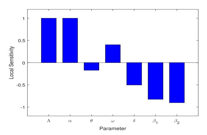
Figure 2: Local sensitivity analysis of R0.
Theorem 6.1. If R0 < 1, then the abstaining-free point E1 is locally asymptotically stable.
Proof: Substituting the abstaining-free equilibrium E1 into the Jacobian matrix in (12), we get a characteristics of the polynomial is
\[C(\lambda) = m_0 \lambda^4 + m_1 \lambda^3 + m_2 \lambda^2 + m_3 \lambda + m_4\] (13)
where
\[\begin{split} m_0 = &1, \\ m_1 = &(1 - R_0) \frac{3\delta + \omega + \theta + \beta_1}{\beta_2 + \delta}, \\ m_2 = &\theta(\beta_1 + \beta_2) + \beta_2(\omega + \beta_1) + 3\delta(2\delta + \omega + \theta + \beta_1 + \beta_2) - \alpha P_{u0}(3\delta + \omega + \theta + \beta_1), \\ m_3 = &\delta^2(4\delta + 3(\omega + \theta + \beta_1 + \beta_2)) + 2\delta(\theta\beta_1 + \beta_2(\theta + \omega)) + \beta_1\beta_2(2\delta + \theta) \\ &- \alpha\delta P_{u1}\left(3\delta + 2(\omega + \theta + \beta_1 + \beta_2)\right), \\ m_4 = &\delta(1 - R_0)(\delta m + \beta_1(\delta + \theta)), \end{split}\]
If and only if R0 < 1 then we get that the values of mi , i = 0, 1, 2, 3, 4 are positive. Further, Re(λi) < 0, i = 1, ..., 4 so that the abstaining-free equilibrium is locally asymptotically stable whenever R0 < 1.
Theorem 6.2. If R0 > 1, then the abstaining point E∗ is exists and locally asymptotically stable.
Proof: Substituting the abstaining equilibrium E∗ into the Jacobian matrix in (12), we get a characteristics of the polynomial is
\[B(\lambda) = g_0 \lambda^4 + g_1 \lambda^3 + g_2 \lambda^2 + g_3 \lambda + g_4\] (14)
where
\[\begin{split} g_0 = & 1, \\ g_1 = & 3\delta + m + \beta_1 + \beta_2 + \alpha(A_* - P_{u*}), \\ g_2 = & A_*\alpha(2\delta + m + \beta_2) + \delta(3\delta + m) + (\beta_1 + \beta_2)(2\delta + m) + \beta_1\beta_2 - \alpha P_{u*}(2\delta + m + \beta_1) - \omega\beta_1, \\ g_3 = & A_*\alpha\delta(\delta + 2m + \beta_2) + A\alpha m\beta_2 + \delta^2(\delta + 3m) + (\beta_1 + \beta_2)(\delta^2 + 2\delta m) + \beta_1\beta_2(\delta + m) + \alpha\omega P_{u*}\beta_1 \\ & - \omega\beta_1(\beta_2 + 2\delta) - \delta\alpha P_{u*}(\delta + 2m) - \alpha\beta_1 P_{u*}(\delta + m), \\ g_4 = & \delta\left[(A_*\alpha m - \omega\beta_1)(\delta + \beta_2) + \delta m(\delta + \beta_1 + \beta_2) + \beta_1(\beta_2 m + \alpha\omega P_{u*}) - P_{u*}\alpha m(\delta + \beta_1)\right]. \end{split}\]
If and only if R0 > 1 then we get that the values of gi , i = 0, 1, 2, 3, 4 are positive. Further, Re(λi) < 0, i = 1, ..., 4 so that the abstaining equilibrium is locally asymptotically stable whenever R0 > 1.
6.2. Global stability
Theorem 6.3. A abstaining-free point \((E_1)\) of the system (1) is globally asymptotically stable for \(R_{0u} < 1\).
Proof: Refer to work by Huo and Zou in [26] and also Ullah et al. in [27], we assume that
\[G_1 = P_{u1}A,\tag{15}\] is a Lyapunov function, where \(P_{u1} = \frac{\Lambda\theta\beta_1}{(\delta m + \beta_1(\delta + \theta))}\). The derivative of the above Lyapunov function gives
\[\frac{dG_1}{dt} = P_{u1} \frac{dA}{dt},\] \[= \frac{\Lambda \theta \beta_1}{(\delta m + \beta_1 (\delta + \theta))} \left[ \alpha P_u A - (\beta_2 + \delta) A \right],\] \[= \frac{\Lambda \theta \beta_1}{(\delta m + \beta_1 (\delta + \theta))} \left[ R_{0u} - \frac{1}{P_u} \right] P_u A.\] (16)
Next, choose \(P_u=1\), we get \(\frac{dG_1}{dt}<0\) if \(R_{0u}<1\). From (10), we have \(R_0>R_{0u}\). Thus, point \(E_1\) is globally asymptotically stable for \(R_{0u}<1\).
Theorem 6.4. If \(R_0 > 1\), the abstaining point \(E_*\) is exists and globally asymptotically stable, while when \(R_0 < 1\) the \(E_*\) is unstable.
Proof: Refer to global proving by [23] and [24], the global stability of System (1) will be analyzed at point \(E_*\) when conditions of \(E_*\) exists and \(R_0 > 1\) are met. The definition and derivation of the Lyapunov function \(G_*\) are as follows:
\[G_* = \frac{1}{2} \left[ (P_u - P_u^*) + (P_a - P_a^*) + (A - A^*) + (R - R^*) \right]^2\] (17)
By differentiating function \(G_*\) in Equation (17) with respect to time for System (1), we have derived the solution given in Equation (18).
\[\frac{dG_*}{dt} = \left[ (P_u - P_u^*) + (P_a - P_a^*) + (A - A^*) + (R - R^*) \right] \frac{dM}{dt}\] (18)
Since \([P_u^*+P_a^*+A+R]=\frac{\Lambda}{\delta}.\) and \(\frac{dM}{dt}=[\Lambda-\delta M]\). it follows that
\[\frac{dG_*}{dt} = \left[ M - \frac{\Lambda}{\delta} \right] \left[ \Lambda - \delta M \right],\] \[= \frac{1}{\delta} \left[ \delta M - \Lambda \right] \left[ \Lambda - \delta M \right],\] \[= -\frac{1}{\delta} \left[ \Lambda - \delta M \right]^2\] (19)
\(\frac{dG_*}{dt}<0\) is a strictly Lyapunov functions as presented in Equation (19). Thus, the abstaining point \(E_*\) is globally asymmtotically stable for \(R_0>1\) in the region \(\Omega\). From Equation (19), \(\frac{dG_*}{dt}=0\) if and only if we set \(P_u=P_u^*, P_a=P_a^*, A=A^*, R=R^*\), and then, \(\frac{dG_*}{dt}\) convergence in positive regions \(\Omega\) as \(t\to\infty\).
7. NUMERICAL SIMULATION
Numerical simulations are conducted in this section to validate the analysis results from the previous section. Using the parameter values from Table 1, we utilized the Fourth-Order Runge-Kutta (RK-4) method to solve System (1). The RK-4 Method is widely used due to its accuracy, precision, and program efficiency. Our theoretical findings are validated with an example and numerical results in this subsection. By utilizing the parameter values in Table 1 and performing calculations, System (1) yields the abstaining point
\[E_* = (0.4382, 1.1906, 0.2968, 3.6132)\]
According to Theorem 6.2 and also Theorem 6.4, point \(E_*\) is asymptotically stable because \(R_0=2.2127>1\) and also every eigenvalue is negative, where: \(\lambda_1=-0.0540, \lambda_2=-0.1937, \lambda_3=-0.1937, \lambda_3=0.1937\) and \(\lambda_4=0.1937\) and \(\lambda_4=0.1937\) and \(\lambda_4=0.1937\) and \(\lambda_4=0.1937\) and \(\lambda_4=0.1937\) and \(\lambda_4=0.1937\) and \(\lambda_4=0.1937\) and \(\lambda_4=0.1937\) and \(\lambda_4=0.1937\) and \(\lambda_4=0.1937\) and \(\lambda_4=0.1937\) and \(\lambda_4=0.1937\) and \(\lambda_4=0.1937\) and \(\lambda_4=0.1937\) and \(\lambda_4=0.1937\) and \(\lambda_4=0.1937\) and \(\lambda_4=0.1937\) and \(\lambda_4=0.1937\) and \(\lambda_4=0.1937\) and \(\lambda_4=0.1937\) and \(\lambda_4=0.1937\) and \(\lambda_4=0.1937\) and \(\lambda_4=0.1937\) and \(\lambda_4=0.1937\) and \(\lambda_4=0.1937\) and \(\lambda_4=0.1937\) and \(\lambda_4=0.1937\) and \(\lambda_4=0.1937\) and \(\lambda_4=0.1937\) and \(\lambda_4=0.1937\) and \(\lambda_4=0.1937\) and \(\lambda_4=0.1937\) and \(\lambda_4=0.1937\) and \(\lambda_4=0.1937\) and \(\lambda_4=0.1937\) and \(\lambda_4=0.1937\) and \(\lambda_4=0.1937\) and \(\lambda_4=0.1937\) and \(\lambda_4=0.1937\) and \(\lambda_4=0.1937\) and \(\lambda_4=0.1937\) and \(\lambda_4=0.1937\) and \(\lambda_4=0.1937\) and \(\lambda_4=0.1937\) and \(\lambda_4=0.1937\) and \(\lambda_4=0.1937\) and \(\lambda_4=0.1937\) and \(\lambda_4=0.1937\) and \(\lambda_4=0.1937\) and \(\lambda_4=0.1937\) and \(\lambda_4=0.1937\) and \(\lambda_4=0.1937\) and \(\lambda_4=0.1937\) and \(\lambda_4=0.1937\) and \(\lambda_4=0.1937\) and \(\lambda_4=0.1937\) and \(\lambda_4=0.1937\) and \(\lambda_4=0.1937\) and \(\lambda_4=0.1937\) and \(\lambda_4=0.1937\) and \(\lambda_4=0.1937\) and \(\lambda_4=0.1937\) and \(\lambda_4=0.1937\) and \(\lambda_4=0.1937\) and \(\lambda_4=0.1937\) and \(\lambda_4=0.1937\) and \(\lambda_4=0.1937\) and \(\lambda_4=0.1937\) and \(\lambda_4=0.1937\) and \(\lambda_4=0.1937\) and \(\lambda_4=0.1937\) and \(\lambda_4=0.1937\) and \(\lambda_4=0.1937\) and \(\lambda_4=0.1937\) and \(\lambda_4=0.1937\) and \(\lambda_4=0.1937\) and \(\lambda_4=0.1937\) and \(\lambda_4=0.1937\) and \(\lambda_4=0.1937\) and \(\lambda_4=0.1937\) and \(\lambda_4=0.1937\) and \(\lambda_4=0.1937\) and \(\lambda_4=0.1937\) and \(\lambda_4=0.1937\) and \(\lambda_4=0.1937\) and \(\lambda_4=0.1937\) and \(\lambda_4=0.1937\) and \(\lambda_4=0.1937\) and \(\lambda_4=0.1937\) and \(\lambda_4=0.1937\) and \(\lambda_4=0.1937\)
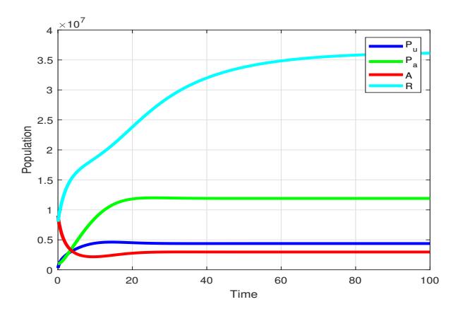
Figure 3: The time series of each class when we set the parameters β1 = β2 = 0.5. The abstainers point E∗ is asymptotically stable.
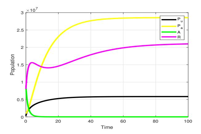
Figure 4: The time series of each class when we set the parameters β1 = β2 = 0.9. The free-abstaining point E1 is asymptotically stable.
−0.7259. This shows that abstaining voters will still exist in the population. Figure 3 illustrates the behavior of this case.
In the next step, the values of the parameter model in Tabel 1 are used consistently, with the sole exception of β1 = β2 = 0.9. The initial conditions match those in the previous scenario. From the calculation results, System (1) has the abstaining-free point
\[E_1(0.5839, 2.8557, 0.0000, 2.0992).\]
Additionally, from Theorem 6.1 and Theorem 6.3, we get free-abstaining point E1 is asymptotically stable because R0 = 0.7739 < 1 and all of the eigenvalues are negative, where: λ1 = −0.0540, λ2 = −0.0902, λ3 = −1.0478, and λ4 = −0.2157. This result shows that there are no abstention voters in the population. Figure 4 depicts the graph relevant to this case.
Furthermore, in Figure 5, the relationship between R0, β1, and β2 was demonstrated by us. With the simultaneous increase of values β1 and β2, the basic reproductive number shows a significant rise. It is evident that increasing awareness campaigns and utilizing argumentative schemes have a notable impact on reducing abstention rates.
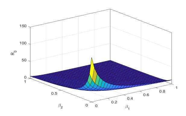
Figure 5: The relationship among \(R_0\), \(\beta_1\), and \(\beta_2\).
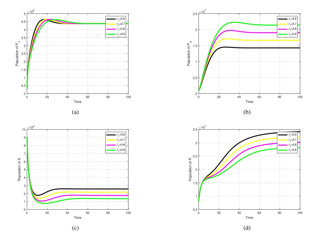
Figure 6: The behavior for each class with various \(\beta_1\).
The increase in values \(\beta_1\) and \(\beta_2\) is in line with the increase in the number of individual conscious voters (see Figures 6b and 7b). This event indicates that awareness campaigns and candidate debates have been confirmed to be able to increase the number of aware voters. Detail in Figures 6c and 7c, the abstentions decrease as the specific parameter values increase in \(\beta_1\) and \(\beta_2\). This means the number of abstaining voters will decrease as awareness campaigns and argumentative schemes increase. The decrease in abstainers impacts the diminishing registry class population. This case is illustrated in Figures 6d and 7d. Thus, through Figures 6a and 7a it shows that unconscious voters still exist in the population. This is related to the chance of voters becoming unconscious again.
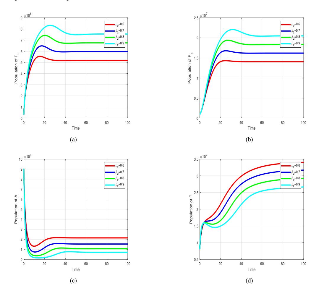
Figure 7: The behavior for each class with various \(\beta_2\).
Educational campaigns seek to enhance individual understanding of their voting rights and encourage active participation in democratic processes. Increased educational campaigns \((\beta_1)\) were confirmed to reduce the reproductive number \((R_0)\) by the analysis results. Likewise, argumentation schemes through candidate debates. The candidate debate that is held will introduce the vision and mission of each candidate. An increase in the value of argumentation scheme \((\beta_2)\) leads to a decrease in the value of reproductive number \((R_0)\). Therefore, a combined strategy of campaign education and argumentative approaches will undoubtedly be the best way to minimize voter absenteeism.
8. Conclusion
This study presents a mathematical model analyzing how citizens register to vote and how abstainers negatively impact potential voters. The Routh-Hurwitz criteria and Lyapunov functions are used to analyze the stability of both abstaining-free and abstaining points, considering both local and global analysis. Additionally, we put forward an optimal approach for an awareness initiative aimed at assisting politicians and officials in boosting citizen registration on electoral lists with the least amount of effort. Next, we implemented two
schemes: the first scheme focused on raising awareness and providing administrative and legal support to encourage potential voters to register on the electoral lists. The second scheme assessed the attempts to engage non-voters through dialogues, debates, and media coverage to encourage their participation in elections.
Based on the formula of R0 in Equation (10), the campaigns rate and effectiveness of argumentative scheme are key factors in decreasing the value of R0. According to the analytical results, for the reproductive number is less than 1, abstaining behavior is controllable. Thus, Model (1) was built based on previous research about a mathematical model for abstinence behavior on the election lists. The simulation incorporated parameter values sourced from an article about a mathematical model for abstinence behavior. Finally, Model (1) can serve as a reference for other voter behavior models, assuming the abstinence behavior is similar.
ACKNOWLEDGEMENT
This research was not funded. We thank the reviewer for his/her suggestions which lead to an improvement of the paper.