

1. Introduction
Coronavirus disease 2019 (COVID-19) is caused by the severe acute respiratory syndrome coronavirus 2 (SARS-CoV-2), first identified in Wuhan, China, in late 2019. The disease rapidly escalated into a global
*Corresponding author
Received March \(13^{th}\), 2024, Revised June \(28^{th}\), 2024 (first), Revised September \(29^{th}\), 2024 (second), Accepted for publication November \(15^{th}\), 2024. Copyright ©2024 Published by Indonesian Biomathematical Society, e-ISSN: 2549-2896, DOI:10.5614/cbms.2024.7.2.2
pandemic, declared by the World Health Organization (WHO) in March 2020, infecting around 776 million confirmed cases resulting in over 7 million deaths [36]. COVID-19 spreads primarily through direct contact with respiratory droplets when an infected person coughs, sneezes, speaks, or breathes [2], [33]. Infected individuals may experience mild to moderate illness, presenting symptoms such as fever, cough, tiredness, and loss of taste or smell. However, individuals with comorbidities or the elderly are more likely to develop severe symptoms such as pneumonia, organ failure, and, in some cases, death [34], [35].
Dengue, a vector-borne disease caused by the Flaviviridae virus, is prevalent in tropical and subtropical regions. It is transmitted through bites from female mosquitoes, primarily Aedes aegypti and Aedes albopictus, and presents symptoms such as high fever, severe headache, muscle and joint pains, vomiting, and rash. Human-to-mosquito transmissions occur when mosquitoes feed on individuals infected with dengue. It is estimated that 390 million dengue virus infections occur per year caused by four distinct virus serotypes–DENV-1, DENV-2, DENV-3, and DENV-4 [3], [37]. Reinfection with a different serotype increases the risk of severe dengue, including dengue hemorrhagic fever. While recovery from a particular serotype provides lifelong immunity to that serotype, reinfection with a different serotype poses a higher risk of developing severe disease, such as dengue hemorrhagic fever (DHF). This challenge, compounded by the lack of a specific cure for dengue, complicates public health management in dengue-endemic regions where vaccination strategies and vector control are key preventive measures [3].
The COVID-19 pandemic has further strained public health systems, particularly in tropical and subtropical regions where dengue is endemic. The overlapping presence of these infectious diseases heightens the risk of co-infection, posing additional diagnostic and treatment challenges, as seen in regions such as Southeast Asia and Latin America.
Cases of COVID-19 and dengue co-infection have been reported in countries such as Brazil [6], India [16], Thailand [25], Pakistan [27], and the Philippines [28]. In many instances, patients initially diagnosed with COVID-19 exhibited low platelet count (thrombocytopenia), low white blood cell count (leukopenia), and liver enzymes were elevated. This is later attributed to concurrent dengue infection. Another case in Thailand [18] where a COVID-19 patient presented with skin rash, a common clinical finding in dengue. In Singapore, two patients were diagnosed with false-positive dengue from rapid serological tests, then subsequently tested positive for COVID-19 [38]. These case reports indicate additional challenges to healthcare systems as COVID-19 and dengue are difficult to distinguish due to overlapping clinical and laboratory features, such as fever, headache, muscle pain or fatigue, nausea, or vomiting [9]. It was also depicted that the co-infection had worse outcomes relative to mortality rate, intensive care unit admission, and prolonged hospital stay [12].
In light of these challenges, deterministic mathematical modeling provides a critical tool for understanding the transmission dynamics of both COVID-19 and dengue, helping guide public health interventions. Using compartmental models described by ordinary differential equations (ODEs), this approach examines disease progression over time, offering insights into potential co-infection scenarios and control strategies. These compartments represent the partition of the population relative to the epidemiological state. Such models were used in forecasting and exploring case scenarios which are essential in formulating policies on optimal strategies for controlling and containing the diseases.
Mathematicians have developed models to study the interactions between different diseases, including coinfections such as tuberculosis-HIV/AIDS [7] and pneumonia-HIV/AIDS [31]. These models have informed effective intervention strategies in resource-limited settings, demonstrating their importance in managing complex health challenges. In the paper of Bakare et al. [5], they formulated a malaria-schistosomiasis co-infection, a parasitic and vector-borne disease model. Furthermore, some studies introduced vector-tovector-borne disease models such as the malaria-lymphatic filariasis [30], dengue-chikungunya [24], and leptospirosis-dengue [1].
During the COVID-19 pandemic, many mathematical models have been developed to project the trajectories of the outbreak and produce optimal interventions to contain the disease. Since different diseases are already prevalent before the pandemic, co-infection with COVID-19 is also present. Several papers were published describing the dynamics of the co-infection of other diseases with COVID-19. The work of Artiono et al. [4] studied the co-infection modeling of COVID-19 and rubella with vaccination treatments for both diseases. Mekonen et al. [22] constructed a COVID-19 and tuberculosis co-infection model. In the study of Hezam et al. [14], optimal control for COVID-19 and cholera co-infection model was analyzed. Similarly, COVID-19- Malaria with vaccination was studied by Shah et al. [29].
Furthermore, a co-endemic model was established by Fahlena et al. [13]. They studied the dynamics of the simultaneous prevalence of COVID-19 and dengue with bifurcation analysis. The model comprises ten compartments for the human population: susceptible individuals, dengue-infected, COVID-19-infected, dengue-infected with COVID-19 immunity, recovered from dengue, recovered from COVID-19, COVID-19-infected with dengue immunity, recovered from both dengue and COVID-19, and two vector compartments: susceptible vectors and dengue-infected vectors. Moreover, there are already existing studies related to the co-infection of COVID-19 and dengue. Hye et al. [15] formulated a seven-compartmental model with optimal control and data-driven analysis in Bangladesh. The model consists of susceptible, dengue-infected, COVID-19-infected, dengue-COVID-19 co-infected, and recovered from disease human compartments, and incorporated disease reinfection. Meanwhile, Omame et al. [26] developed an eight-compartmental co-infection model with optimal control and cost-effectiveness analysis in Brazil.
In this study, we modify and integrate the models formulated in [13], [15] into a new COVID-19-dengue co-infection model. This paper will discuss the model formulation and its well-posedness in Section 2. Section 3 will cover the calculation of equilibrium point, reproduction numbers, and stability analysis. In Section 4, numerical simulations are presented. Lastly, Section 5 establishes the conclusions.
2. MODEL FORMULATION
This study builds upon the model developed by Fahlena \(\it{et\,al.}\) [13] which examines the co-endemic dynamics of COVID-19 and dengue. The model is further expanded by incorporating the co-infection compartment and recovery rates established by Hye \(\it{et\,al.}\) [15], allowing for a more comprehensive analysis of the interactions between the two diseases. The compartmental diagram of the co-infection model is illustrated in Figure 1, with state variables described in Table 1. The model assumes a homogeneous or well-mixed population where host and vector population growth follow arithmetic recruitment rates. For simplicity, the model considers only one dengue serotype (transmitted by \(\it{Aedes\,aegypti}\)) and one COVID-19 variant, acknowledging that this represents a limited case of the full disease dynamics. Individuals who recover from either COVID-19 or dengue acquire lifetime immunity to the respective disease. The model assumes that neither disease is transmitted by birth. Furthermore, co-infected individuals in compartment \(\it{I}_{\it{x}}\) are quarantined and closely monitored, preventing them from transmitting either disease. This assumption aligns with real-world isolation practices for managing severe co-infections, ensuring that both diseases are contained during the recovery period.
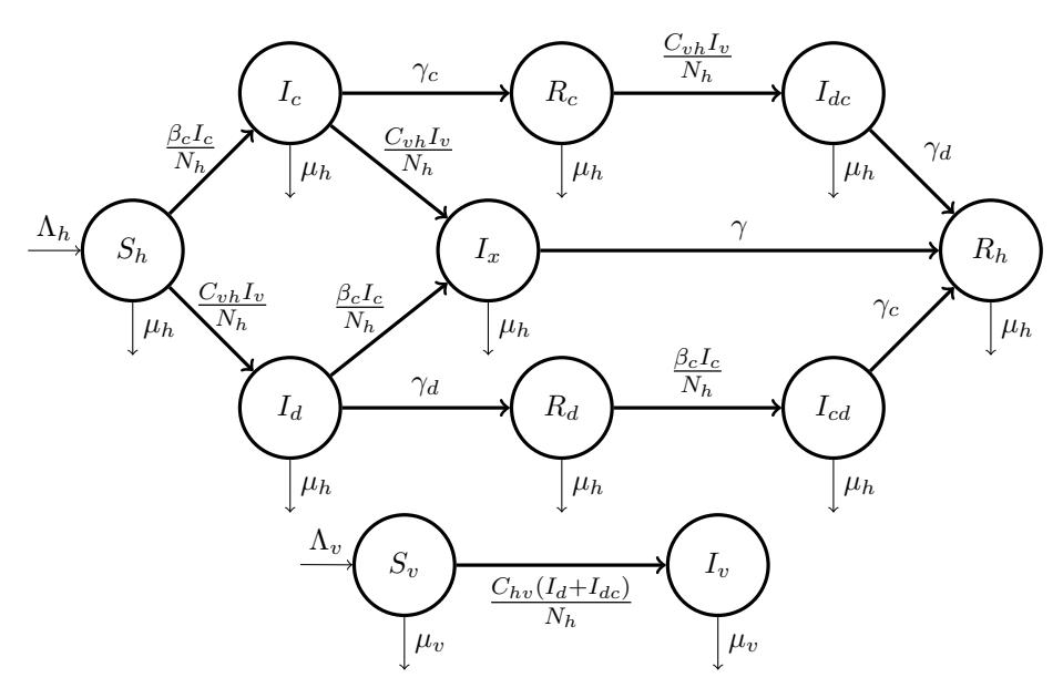
Figure 1: COVID-19 and dengue co-infection model diagram.
Table 1: Model state variable description.
| State V | Variables | Description |
|---|---|---|
| \(\overline{S_i}\) | h(t) | Number of susceptible individuals at time \(t\) |
| \(S_{i}\) | \(_{v}(t)\) | Number of susceptible vectors at time t |
| \(I_{c}\) | \(_{c}(t)\) | Number of COVID-19-infected individuals at time \(t\) |
| \(I_{c}\) | \(_{l}(t)\) | Number of dengue-infected individuals at time t |
| \(I_i\) | ,(t) | Number of dengue-infected vectors at time t |
| \(I_c\) | \(_{d}(t)\) | Number of COVID-19-infected individuals with dengue immunity at time \(t\) |
| \(I_d\) | \(_{c}(t)\) | Number of dengue-infected individuals with COVID-19 immunity at time \(t\) |
| \(_{c}(t)\) | Number of COVID-19-dengue co-infection individuals at time \(t\) | |
| R | \(_{c}(t)\) | Number of COVID-19 recovered individuals at time \(t\) |
| R | \(_{d}(t)\) | Number of dengue recovered individuals at time t |
| \(R_{i}\) | h(t) | Number of individuals recovered in both COVID-19 and dengue at time \(t\) |
Table 2: Model parameter description.
| Parameter | Description | Value | Unit | Reference |
|---|---|---|---|---|
| \(\Lambda_h\) | Human recruitment rate | 1500 | Individual | Assumed |
| \(\Lambda_v\) | Vectors recruitment rate | 10000 | Mosquito | Assumed |
| \(\beta_c\) | COVID-19 transmission coefficient | [0, 1] | \(day^{-1}\) | [13] |
| \(C_{vh}\) | Dengue transmission coefficient from vector to human | [0, 1] | \(day^{-1}\) | [13] |
| \(C_{vh}\) | Dengue transmission coefficient from human to vector | 0.5 | \(day^{-1}\) | Assumed |
| \(\mu_h\) | Human mortality rate | 0.003 | \(day^{-1}\) | Assumed |
| \(\mu_v\) | Vector mortality rate | 0.01 | \(day^{-1}\) | [26] |
| \(\gamma_c\) | Recovery rate from COVID-19 | 1/14 | \(day^{-1}\) | [13] |
| \(\gamma_d\) | Recovery rate from Dengue | 1/14 | \(day^{-1}\) | [26] |
| \(N_h(0)\) | Human population (initial value) | 500000 | Individual | Assumed |
\[\frac{dS_h}{dt} = \Lambda_h - \left(C_{vh} \frac{I_v}{N_h} + \beta_c \frac{I_c}{N_h} + \mu_h\right) S_h, \frac{dI_d}{dt} = C_{vh} \frac{S_h I_v}{N_h} - \left(\beta_c \frac{I_c}{N_h} + \gamma_d + \mu_h\right) I_d, \frac{dR_d}{dt} = \gamma_d I_d - \left(\beta_c \frac{I_c}{N_h} + \mu_h\right) R_d, \frac{dI_{dc}}{dt} = C_{vh} \frac{R_c I_v}{N_h} - (\gamma_d + \mu_h) I_{dc}, \frac{dI_c}{dt} = \beta_c \frac{S_h I_c}{N_h} - \left(C_{vh} \frac{I_v}{N_h} + \gamma_c + \mu_h\right) I_c, \frac{dR_c}{dt} = \gamma_c I_c - \left(C_{vh} \frac{I_v}{N_h} + \mu_h\right) R_c, \frac{dI_{cd}}{dt} = \beta_c \frac{R_d I_c}{N_h} - (\gamma_c + \mu_h) I_{cd}, \frac{dI_d}{dt} = C_{vh} \frac{I_v I_c}{N_h} + \beta_c \frac{I_c I_d}{N_h} - (\gamma_c + \mu_h) I_x, \frac{dR_h}{dt} = \gamma_c I_{cd} + \gamma_d I_{dc} + \gamma I_x - \mu_h R_h, \frac{dS_v}{dt} = \Lambda_v - \left(C_{hv} \frac{I_d + I_{dc}}{N_h} + \mu_v\right) S_v, \frac{dI_v}{dt} = C_{hv} \frac{(I_d + I_{dc}) S_v}{N_h} - \mu_v I_v.\] (1)
The growth equations for the human and vector populations are given by \(dN_h/dt = \Lambda_h - \mu_h N_h\) and \(dN_v/dt = \Lambda_v - \mu_v N_v\), respectively. These equations assume constant recruitment rates \(\Lambda_h\) and \(\Lambda_v\), reflecting stable birth rates and neglecting the impact of other demographic factors such as migration or environmental changes. The system of 11 nonlinear ODEs (1) captures the net rate of change for each epidemiological compartment.
The well-posedness of the model ensures that the system of ODEs has a unique solution for any valid initial condition. This property is crucial for verifying both the mathematical consistency and the biological relevance of the model. The well-posedness guarantees that small changes in initial conditions do not lead to chaotic outcomes, ensuring the robustness of the model's predictions. The theorem from [17] is applied to demonstrate the well-posedness of the COVID-19-dengue co-infection model.
Theorem 2.1. [17] Let f(t,x) be piecewise continuous in t and locally Lipschitz in x for all \(t \ge t_0\) and all x in domain \(D \subset \mathbb{R}^n\). Let W be a compact subset of D, \(x_0 \in W\), and suppose it is known that every solution of
\[\dot{x} = f(t, x), \quad x(t_0) = x_0.\]
lies in W. Then, there is a unique solution that is defined for all \(t \geq t_0\).
The succeeding theorems for the feasibility region and nonnegativity of solutions follow the proof structures in [20], [21].
Theorem 2.2 (Feasible Region). For all \(t \ge 0\), the compact feasible region of the system (1) is the space
\[\Phi = \Phi_h \times \Phi_v\] where
\[\begin{split} & \Phi_h = \left\{ \left( S_h, I_d, R_d, I_{dc}, I_c, R_c, I_{cd}, R_h, I_x \right) \ \middle| \ 0 \leq N_h \leq \max \left\{ \Delta_h, \frac{\Lambda_h}{\mu_h} + \epsilon_h \right\} \right\}, \\ & \Phi_v = \left\{ \left( S_h, I_v \right) \ \middle| \ 0 \leq N_v \leq \max \left\{ \Delta_v, \frac{\Lambda_v}{\mu_v} + \epsilon_v \right\} \right\}, \\ & \Delta_h = \max \left\{ N_h(t) \ \middle| \ 0 \leq t \leq \infty \right\}, \qquad \Delta_v = \max \left\{ N_v(t) \ \middle| \ 0 \leq t \leq \infty \right\}. \end{split}\]
Proof: From system (1),
\[\frac{dN_h}{dt} = \Lambda_h - \mu_h N_h,\]\[\frac{dN_v}{dt} = \Lambda_v - \mu_v N_v,\] are linear ODEs, and the following are its respective solutions.
\[\begin{split} N_h(t) &= \frac{N_h(0)}{e^{\mu_h t}} + \frac{\Lambda_h}{\mu_h}, \\ N_v(t) &= \frac{N_v(0)}{e^{\mu_v t}} + \frac{\Lambda_v}{\mu_v}. \end{split}\]
Thus, the \(\lim_{t\to\infty}N_h(t)=\frac{\Lambda_h}{\mu_h}\). Moreover, for some sufficiently small \(\epsilon_h\), there exists some sufficiently large T>0 such that the limit supremum \(N_h(t)=\frac{\Lambda_h}{\mu_h}+\epsilon_h\) for all t>T. Furthermore, we have \(\Delta_h=\sup_{0< t\leq \infty}N_h(t)\)
such that
\[N_h \le \max \left\{ \Delta_h, \frac{\Lambda_h}{\mu_h} + \epsilon_h \right\}.\] for all \(t \geq 0\). Similar argument applies to \(N_v\).
Theorem 2.3 (Nonnegativity of the Solutions). Each solution of system (1) with initial condition in the hyper-octant \(\mathbb{R}^{11}_{0,+}\), must also be in \(\mathbb{R}^{11}_{0,+}\).
Proof: From the first equation in (1),
\[\frac{dS_h}{dt} = \Lambda_h - (C_{vh}I_v + \beta_c I_c) \frac{S_h}{N_h} - \mu_h S_h,\]\[\geq - (C_{vh}I_v + \beta_c I_c) \frac{S_h}{N_h} - \mu_h S_h,\]
since the recruitment rate \(\Lambda_h \geq 0\). Now, let \(u(t) = -\left(\frac{C_{vh}I_v + \beta_cI_c}{N_h} - \mu_h\right)\), the inequality above becomes
\[\frac{dS_h}{dt} \ge u(t)S_h. \tag{2}\]
Define \(g(t) = \exp\left(\int_0^t u(r)dr\right)\). Observe that g(t) > 0 for all values of t. Taking the derivative of g with
\[\frac{d}{dt}g(t) = \exp\left(\int_0^t u(r)dr\right) \frac{d}{dt} \int_0^t u(r)dr.\]
By the Fundamental Theorem of Calculus, this differential equation becomes
\[\frac{d}{dt}g(t) = g(t) \ u(t).\]
As we compute the derivative of \(\frac{S_h(t)}{q(t)}\), the inequality (2) is utilized which leads to
\[\frac{d}{dt} \left( \frac{S_h(t)}{g(t)} \right) = \frac{g(t) \frac{d}{dt} S_h(t) - S_h(t) \frac{d}{dt} g(t)}{[g(t)]^2} \\ \ge \frac{g(t) u(t) S_h(t) - S_h(t) g(t) u(t)}{[g(t)]^2} = 0.\]
This implies that \(\frac{S_h(t)}{g(t)}\) is nondecreasing for any values of t.
Now,
\[\frac{S_h(t)}{g(t)} \ge \frac{S_h(0)}{g(0)} = S_h(0),\] which simplifies to
\[S_h(t) \ge S_h(0) \ g(t) \ge 0.\]
Hence, \(S_h(t)\) is nonnegative for all \(t \ge 0\).
Similarly, from equation 2 in (1), we deduce this to
\[\frac{dI_d}{dt} = C_{vh} \frac{I_v}{N_h} S_h - \beta_c I_c \frac{I_d}{N_h} - (\gamma_d + \mu_h) I_d\]\[\geq -\beta_c I_c \frac{I_d}{N_h} - (\gamma_d + \mu_h) I_d.\]
The rate \(C_{vh} \frac{I_v}{N_h} S_h \ge 0\) since this term is the number of individuals coming from susceptible \(S_h\) compartment into the dengue-infected \(I_d\) compartment, furthermore, this quantity will not be negative as infected can not transfer back directly to the susceptible compartment. Following from the same argument above, we have
\[I_d \ge I_d(0) \exp \left[ -\int_0^t \left( \frac{\beta_c I_c}{N_h} + \gamma_d + \mu_h \right) dr \right] \ge 0.\]
The same argument applies to other state variables for all \(t \ge 0\). Hence, all solutions of the system of ODEs are nonnegative.
Theorem 2.4 (Well-posedness of the model system). For each initial condition
\[\mathbf{x}(0) = (S_h(0), I_d(0), I_d(0), I_{dc}(0), I_c(0), R_c(0), I_{cd}(0), I_x(0), R_h(0), S_v(0), I_v(0)) \in \Phi,\] the solution to the model system (1) in \(\Phi\) exists and is unique.
Proof.
- (1) Continuity. It can be observed that the model system is continuous since each ODE is a polynomial function of time t.
- (2) Local Lipschitz condition. Instead of solving each \([\partial f/\partial x](t,x)\) for all state variables, we can present this through the Jacobian matrix \(\mathbf{J}(\mathbf{x})\) of the system. The entries of this matrix are all linear relative to its respective state variable with constant positive parameters which include \(N_h\) and \(N_v\).
- (3) Invariance over a compact feasible region. Shown in Theorem 2.2, the compact feasible region of the model was defined as \(\Phi\). Furthermore, Theorem 2.3 proved the nonnegativity invariance of each model compartment. This invariance property will then be carried in the region \(\Phi\) as \(\Phi \subset \mathbb{R}^{11}_{0,+}\).
Hence, by Theorem 2.1, the model system (1) is well-posed.
3. MODEL ANALYSIS
This section outlines the calculation of the four equilibrium points of system (1) which correspond to key states in the co-infection dynamics: the disease-free state, COVID-19-only state, dengue-only state, and co-infection state. The existence and local stability of these points are analyzed, with the assumption that the total populations \(N_h\) and \(N_v\) are constant. It follows that the parameters \(\Lambda_h\), \(\Lambda_v\) represent \(\mu_h N_h\), \(\mu_v N_v\), respectively. These analyses are conducted with the aid of MATLAB R2023b and Maple software. Additionally, the basic reproduction number \(\mathcal{R}_0\), a quantity that represents the average number of new infections caused by a single infectious individual in a completely susceptible population, is derived using the Next Generation Matrix (NGM) method developed by Diekmann et al. [11].
3.1. Disease-free equilibrium and basic reproduction number
The disease-free equilibrium represents the steady-state solution of system (1) where neither COVID-19 nor dengue persists in human or vector populations. This equilibrium is a critical baseline in epidemiological models, as it indicates the conditions under which both diseases are eradicated from the population, and no further transmission occurs.
To calculate the equilibrium, we set all ODEs in system (1) to zero and assume that there are no infected individuals (\(I_d = R_d = I_{dc} = I_c = R_c = I_{cd} = I_v = I_x = R_h = 0\)). By solving for the state variables, we determine the steady-state solution where no new infections occur, representing the complete eradication of both diseases. Denoted as \(E_0\), the resulting equilibrium is given by
\[E_{0} = \left(S_{h}^{0}, I_{d}^{0}, R_{d}^{0}, I_{dc}^{0}, I_{c}^{0}, R_{c}^{0}, I_{cd}^{0}, I_{x}^{0}, R_{h}^{0}, S_{v}^{0}, I_{v}^{0}\right)\] \[= \left(\frac{\Lambda_{h}}{\mu_{h}}, 0, 0, 0, 0, 0, 0, 0, \frac{\Lambda_{v}}{\mu_{v}}, 0\right).\] (3)
The equilibrium \(E_0\) exists for any positive parameter values. Using the Next Generation Matrix (NGM) method, we calculate the basic reproduction number \(\mathcal{R}_0\), a crucial indicator of disease transmission. The value of \(\mathcal{R}_0\) serves as a key threshold: if \(\mathcal{R}_0 < 1\), the disease will die out, while if \(\mathcal{R}_0 > 1\), it will continue to spread [32].
Theorem 3.1 (Basic Reproduction Number). The basic reproduction number \(\mathcal{R}_0\) of system (1) is calculated as
\[\mathcal{R}_0 = \max \left\{ \mathcal{R}_{0c}, \mathcal{R}_{0d} \right\},\,\] where \(\mathcal{R}_{0c}\) represents the reproduction number for COVID-19, and \(\mathcal{R}_{0d}\) represents the reproduction number for dengue. Specifically,
\[\mathcal{R}_{0c} = \frac{\Lambda_h \beta_c}{N_h \mu_h (\mu_h + \gamma_c)}, \quad \text{describes the spread of COVID-19; and}\] \[\mathcal{R}_{0d} = \frac{1}{N_h \mu_v} \sqrt{\frac{\Lambda_h \Lambda_v C_{vh} C_{hv}}{\mu_h (\mu_h + \gamma_d)}}, \quad \text{describes dengue dynamics, including its vector-borne nature.}\] (4)
Proof: By the NGM method, we only need the infected compartments \(I_d\), \(I_c\), \(I_{cd}\), \(I_{dc}\), \(I_x\), \(I_v\) to find the transfer matrix V and incidence matrix F. These matrices have been obtained from the Jacobian matrix of the said infected compartments, these are as follows
\[\text{[rumus tidak dapat ditampilkan dengan baik — lihat PDF asli]}\]
Then, matrix F has been evaluated at equilibrium \(E_0\)
\[\text{[rumus tidak dapat ditampilkan dengan baik — lihat PDF asli]}\]
Now, the NGM has been calculated as
\[\text{[rumus tidak dapat ditampilkan dengan baik — lihat PDF asli]}\]
Solving for the spectral radius of the NGM, that is the eigenvalues of the matrix, this results into two positive eigenvalues \(\mathcal{R}_{0c}\) and \(\mathcal{R}_{0d}\) as shown in (4). The eigenvalue \(\mathcal{R}_{0c}\) is expressed in COVID-19 parameters, while \(\mathcal{R}_{0d}\) in dengue parameters. Hence, these eigenvalues are denoted as the basic reproduction number for COVID-19 and dengue, respectively. Moreover, one can be larger than the other, for some parameter values, thus, we take the maximum.
Theorem 3.2 (Stability of Disease-free Equilibrium). The Disease-free Equilibrium \(E_0\) is locally asymptotically stable if \(\mathcal{R}_0 < 1\). Otherwise, \(E_0\) is unstable.
Proof: Using the linearization method, the Jacobian matrix of system (1) evaluated at \(E_0\) is given as
\[\text{[rumus tidak dapat ditampilkan dengan baik — lihat PDF asli]}\]
Hereafter, we get the resulting characteristic polynomial \(P_0(\lambda)\) of matrix \(\mathbf{J}(E_0)\)
\[P_0(\lambda) = (\mu_h + \lambda)^4 (\mu_v + \lambda)(\gamma_c + \mu_h + \lambda)(\gamma_d + \mu_h + \lambda)(\gamma + \mu_h + \lambda) \left[\lambda + (\mu_h + \gamma_c)(1 - \mathcal{R}_{0c})\right] \left[\lambda^2 + (\mu_h + \mu_v + \gamma_d)\lambda + \mu_v(\mu_d + \gamma_d)(1 - \mathcal{R}_{0d}^2)\right].\]
It can be observed that the product
\[(\mu_h + \lambda)^4 (\mu_v + \lambda)(\gamma_c + \mu_h + \lambda)(\gamma_d + \mu_h + \lambda)(\gamma + \mu_h + \lambda),\]
gives us negative eigenvalues for positive parameter values. Similarly, the factor \(\lambda + (\mu_h + \gamma_c)(1 - \mathcal{R}_{0c})\) has negative eigenvalues only if \(\mathcal{R}_{0c} < 1\). Meanwhile, by the Routh-Hurwitz criterion, the quadratic equation
\[\lambda^{2} + (\mu_{h} + \mu_{v} + \gamma_{d})\lambda + \mu_{v}(\mu_{d} + \gamma_{d})(1 - \mathcal{R}_{0d}^{2}) = 0,\]
has roots of negative real part if the term \(\mu_v(\mu_d + \gamma_d)(1 - \mathcal{R}_{0d}^2) > 0\), that happens only when \(\mathcal{R}_{0d} < 1\). Thus, if \(\mathcal{R}_{0c}\), \(\mathcal{R}_{0d} < 1\), then all eigenvalues of the characteristic polynomial \(P_0(\lambda)\) have negative real part. We conclude that the disease-free equilibrium \(E_0\) is locally asymptotically stable if \(\mathcal{R}_{0c}\), \(\mathcal{R}_{0d} < 1\). Otherwise, unstable.
3.2. COVID-19-only equilibrium
The COVID-19-only equilibrium is the steady-state solution of system (1) where only COVID-19 persists, and no dengue-infected individuals and vectors. To calculate the equilibrium, we let the initial population in the compartments \(I_d = R_d = I_{dc} = I_v = I_x = R_h = 0\). This equilibrium is denoted as \(E_1^*\), in particular
\[E_1^* = (S_h^*, I_d^*, R_d^*, I_{dc}^*, I_c^*, R_c^*, I_{cd}^*, I_x^*, R_h^*, S_v^*, I_v^*),\] (5)
where
\[S_{h}^{*} = \frac{\Lambda_{h}}{\mathcal{R}_{0c}\mu_{h}}, \quad I_{d}^{*} = 0, \quad R_{d}^{*} = 0, \quad I_{dc}^{*} = 0,\] \[I_{c}^{*} = \frac{(\mathcal{R}_{0c} - 1)N_{h}\mu_{h}}{\beta_{c}},\] \[R_{c}^{*} = \frac{(\mathcal{R}_{0c} - 1)N_{h}\gamma_{c}}{\beta_{c}},\] \[I_{cd}^{*} = 0, \quad I_{x}^{*} = 0, \quad R_{h}^{*} = 0,\] \[S_{v}^{*} = \frac{\Lambda_{v}}{\mu_{v}}, \quad I_{v}^{*} = 0.\] \[(6)\]
Certainly, the equilibrium \(E_1^*\) exists if \(\mathcal{R}_{0c} > 1\). Furthermore, the stability of the equilibrium will be discussed in the following theorem.
Theorem 3.3 (Stability of COVID-19-only Equilibrium). The equilibrium \(E_1^*\) is locally stable if
\[\mathcal{R}_{0c} > 1\] and \(\mathcal{R}_{0d}^2 < \min\{z_1, z_2\}\), where
\[\text{[rumus tidak dapat ditampilkan dengan baik — lihat PDF asli]}\] \[\text{[rumus tidak dapat ditampilkan dengan baik — lihat PDF asli]}\] \[z_{2} = \frac{\mu_{h} + \gamma_{c}}{(\gamma_{d} + \mu_{h})\gamma_{c}\beta_{c}N_{h} \Big[ (\mathcal{R}_{0c} - 1)\mu_{h} + \gamma_{d} \Big]\mu_{v}^{2}} \Big[ N_{h}\beta_{c}\mu_{v}^{2}(\gamma_{d} + \mu_{h}) \cdot \Big]\] \[(\mathcal{R}_{0c}\mu_{h} + \gamma_{d}) - \mu_{h}(\gamma_{c} + \gamma_{d} + \mu_{h})\Lambda_{v}C_{hv}C_{vh} \Big].\] \[(7)\]
Otherwise, \(E_1^*\) is unstable.
Proof: Customarily, the system's Jacobian matrix evaluated at \(E_1^*\) will result to the characteristic polynomial \(P_c(\lambda)\), and is given by
\[P_c(\lambda) = (\mu_h + \lambda)^2 (\mu_v + \lambda)(\gamma_c + \mu_h + \lambda)(\gamma + \mu_h + \lambda) (\mathcal{R}_{0c}\mu_h + \lambda) (\lambda^2 + a_1\lambda + a_2)(\lambda^3 + b_1\lambda^2 + b_2\lambda + b_3),\] where
\[\begin{split} a_1 &= \mu_h \mathcal{R}_{0c}, \\ a_2 &= \mu_h (\mu_h + \gamma_c) \big( \mathcal{R}_{0c} - 1 \big), \\ b_1 &= \mathcal{R}_{0c} \mu_h + 2 \gamma_d + \mu_h + \mu_v, \\ b_2 &= \frac{1}{N_h (\gamma_c + \mu_h) \beta_c \mu_v} \Big[ N_h \mu_v \Big( \big\{ (\mathcal{R}_{0c} + 1) \mu_h^2 + \big[ (-\mathcal{R}_{0d}^2 + \mathcal{R}_{0c} + 1) \gamma_c + 2 \gamma_d \big] \mu_h \\ &- \gamma_c \gamma_d (\mathcal{R}_{0d}^2 - 2) \big\} \mu_v + (\gamma_d + \mu_h) (\mathcal{R}_{0c} \mu_h + \gamma_d) (\gamma_c + \mu_h) \Big) \beta_c - \Lambda_v C_{hv} C_{vh} \mu_h (\gamma_c + \mu_h) \Big], \\ b_3 &= \frac{1}{N_h (\gamma_c + \mu_h) \beta_c \mu_v} \Big( (N_h \mathcal{R}_{0c} \beta_c \mu_v^2 - \Lambda_v C_{hv} C_{vh}) \mu_h^3 - \big\{ \big[ (\mathcal{R}_{0c} \mathcal{R}_{0d}^2 - \mathcal{R}_{0d}^2 - \mathcal{R}_{0c}) \gamma_c \\ &- \gamma_d (\mathcal{R}_{0c} + 1) \big] \mu_v^2 N_h \beta_c + (2 \gamma_c + \gamma_d) C_{hv} \Lambda_v C_{vh} \big\} \mu_h^2 - \big\{ \mu_v^2 \big[ (\mathcal{R}_{0c} \mathcal{R}_{0d}^2 - \mathcal{R}_{0c} - 1) \gamma_c \\ &- \gamma_d \big] N_h \gamma_d \beta_c + \Lambda_v \gamma_c C_{hv} C_{vh} (\gamma_d + \gamma_c) \big\} \mu_h - \gamma_c \gamma_d^2 N_h \mu_v^2 \beta_c (\mathcal{R}_{0d}^2 - 1) \Big). \end{split}\]
It can be observed that the equation
\[(\mu_h + \lambda)^2 (\mu_v + \lambda)(\gamma_c + \mu_h + \lambda)(\gamma + \mu_h + \lambda)(\mathcal{R}_{0c}\mu_h + \lambda) = 0,\]
results to negative eigenvalues for any positive parameter values.
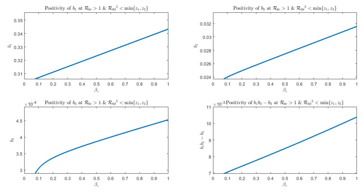
Figure 2: Numerical simulations for Routh-Hurwitz of \(\lambda^3 + b_1 \lambda^2 + b_2 \lambda + b_3\) at \(\mathcal{R}_{0c} > 1\) & \(\mathcal{R}_{0d}^2 < \min\{z_1, z_2\}\).
Moreover, by the Routh-Hurwitz criterion for the factor \(\lambda^2 + a_1\lambda + a_2\) has two eigenvalues with negative real part, whenever \(a_1, a_2 > 0\), and this will be true only if \(\mathcal{R}_{0c} > 1\). In addition, since \(b_1\) is already positive, and by the Routh-Hurwitz criterion for expression \(\lambda^3 + b_1\lambda^2 + b_2\lambda + b_3\), negative eigenvalues are possible if \(\mathcal{R}_{0d}^2 < z_1\) to satisfy \(b_2 > 0\), and \(\mathcal{R}_{0d}^2 < z_2\) for \(b_3 > 0\). To satisfy both coefficients \(b_1, b_2 > 0\), we take the solution set of values for \(\mathcal{R}_{0d}\), that is the minimum of either \(z_1, z_2\) which is the upper bound for \(\mathcal{R}_{0d}^2\).
Furthermore, we assume that the Routh-Hurtwitz inequality \(b_1b_2 > b_3\) is true such that this condition has been supported numerically using Monte-Carlo simulation as illustrated in Figure 2. Hence, considering all inequalities and conditions established, the COVID-19-only equilibrium \(E_1^*\) is stable, if \(\mathcal{R}_{0c} > 1\) and \(\mathcal{R}_{0d}^2 < \min\{z_1, z_2\}\). Otherwise, \(E_1^*\) is unstable.
3.3. Dengue-only equilibrium
The dengue-only equilibrium is the steady-state solution of System (1) where only dengue persists among the populations and there are no COVID-19-infected individuals. To calculate the equilibrium, we let the initial population in the compartments \(I_d = R_d = I_{dc} = I_x = R_h = 0\). This is denoted as \(E_2^{**}\), and is given by
\[E_2^{**} = (S_h^{**}, I_d^{**}, R_d^{**}, I_{dc}^{**}, I_c^{**}, R_c^{**}, I_{cd}^{**}, I_r^{**}, R_h^{**}, S_n^{**}, I_n^{**}), \tag{8}\]
\[S_h^{**} = \frac{\mu_v N_h \left[ N_h (\gamma_d + \mu_h) \mu_v + \Lambda_h C_{hv} \right]}{C_{hv} (N_h \mu_h \mu_v + \Lambda_v C_{vh})},\] \[I_d^{**} = \frac{N_h^2 \mu_v^2 \mu_h (\mathcal{R}_{0d}^2 - 1)}{C_{hv} (N_h \mu_h \mu_v + \Lambda_v C_{vh})},\] \[R_d^{**} = \frac{\gamma_d N_h^2 \mu_v^2 (\mathcal{R}_{0d}^2 - 1)}{C_{hv} (N_h \mu_h \mu_v + \Lambda_v C_{vh})},\] \[I_{dc}^{**} = 0, \quad I_c^{**} = 0, \quad R_c^{**} = 0, \quad I_{cd}^{**} = 0, \quad I_x^{**} = 0, \quad R_h^{**} = 0,\] \[(9)\]
\[S_{v}^{**} = \frac{N_{h}(\gamma_{d} + \mu_{h})(N_{h}\mu_{h}\mu_{v} + \Lambda_{v}C_{vh})}{C_{vh}[N_{h}(\gamma_{d} + \mu_{h})\mu_{v} + \Lambda_{h}C_{hv}]},\] \[I_{v}^{**} = \frac{\mu_{v}N_{h}^{2}\mu_{h}(\gamma_{d} + \mu_{h})(\mathcal{R}_{0d}^{2} - 1)}{C_{vh}[N_{h}(\gamma_{d} + \mu_{h})\mu_{v} + \Lambda_{h}C_{hv}]}.\]
Clearly, the equilibrium \(E_2^{**}\) exists if only \(\mathcal{R}_{0d} > 1\).
Theorem 3.4 (Stability of Dengue-only Equilibrium). The equilibrium \(E_2^{**}\) is locally stable if
\[\mathcal{R}_{0d} > 1\] and \(\mathcal{R}_{0c} < z_3\), where
\[z_{3} = \frac{1}{\mu_{h}C_{hv}(\mu_{h} + \gamma_{c})\left[2N_{h}(\gamma_{d} + \mu_{h})\mu_{v} + \Lambda_{h}C_{hv}\right]} \left(\mu_{h}\Lambda_{h}C_{hv}^{2}(\mu_{h} + \gamma_{c}) + C_{hv}(\gamma_{d} + \mu_{h})\left\{2N_{h}\mathcal{R}_{0d}^{2}\mu_{h}^{2}\mu_{v} + \mu_{h}\left[\gamma_{c}\mu_{v}N_{h}(\mathcal{R}_{0d}^{2} + 1) + \Lambda_{v}C_{vh}\mathcal{R}_{0d}^{2}\right] + \Lambda_{v}C_{vh}\gamma_{c}\right\} - \mu_{v}^{2}\beta_{c}N_{h}(\gamma_{d} + \mu_{h})^{2}\right).\] \[(10)\]
Otherwise, \(E_2^{**}\) is unstable.
Proof: Customarily, the Jacobian matrix of System (1) evaluated at \(E_2^{**}\) will result to the characteristic polynomial
\[P_d(\lambda) = (\lambda + \mu_h)^2 (\lambda + \mu_v)(\lambda + \gamma_c + \mu_h)(\lambda + \gamma_d + \mu_h)(\lambda + \gamma + \mu_h)\]\[(c_0\lambda + c_1)(d_0\lambda + d_1)(\lambda^3 + e_1\lambda^2 + e_2\lambda + e_3).\]
See Appendix 1 for the expressions of the coefficients \(c_0\), \(c_1\), \(d_0\), \(d_1\), \(e_1\), \(e_2\), \(e_3\). It can be observed that the product
\[(\lambda + \mu_h)^2 (\lambda + \mu_v)(\lambda + \gamma_c + \mu_h)(\lambda + \gamma_d + \mu_h)(\lambda + \gamma + \mu_h),\]
gives negative eigenvalues for any positive parameter values. For \(c_0\), \(c_1 > 0\), then factor \((c_0\lambda + c_1)\) results to a negative eigenvalue \(\lambda = \frac{-c_1}{c_0}\). In \((d_0\lambda + d_1)\), we also have \(d_0 > 0\) for positive parameter values. Furthermore, by analytical calculation of the coefficient \(d_1 > 0\), if \(\mathcal{R}_{0c} < z_3\). Therefore, the resulting eigenvalue \(\lambda = \frac{-d_1}{d_0}\) is also negative.
Similarly, the coefficients \(e_1\), \(e_2\), \(e_3\) are positive if \(\mathcal{R}_{0d}\) is greater than unity which supports one of the conditions for \(E_2^{**}\) to exist. Furthermore, we assume the Routh-Hurwitch condition \(e_1e_2-e_3>0\) to be true. This condition has been supported numerically for \(\mathcal{R}_{0d}>1\) using Monte-Carlo simulation as illustrated in Figure 3. Thus, the expression \(\lambda^3+e_1\lambda^2+e_2\lambda+e_3\) has all eigenvalues with negative real parts if \(\mathcal{R}_{0d}>1\).
This concludes that the dengue-only equilibrium \(E_2^{**}\) is locally asymptotically stable if \(\mathcal{R}_{0d} > 1\) and Inequality (10) is satisfied. Otherwise, unstable.
3.4. COVID-19-dengue co-infection equilibrium
The COVID-19-dengue co-infection equilibrium is the steady-state solution of the system (1) where both diseases exist and persist among the human and vector populations. Similarly, individuals may contract these diseases concurrently. Since solving for this equilibrium point does not give analytical closed solution, we resorted to parameterize the state variable \(I_v\) along with the other parameters. Thus, the co-infection equilibrium point, denoted as \(E_3^{***}\), is given by
\[E_3^{***} = (S_h^{***}, I_d^{***}, R_d^{***}, I_{dc}^{***}, I_c^{***}, R_c^{***}, I_{cd}^{***}, I_r^{***}, R_h^{***}, S_n^{***}).\]
See Appendix 2 for the complete details of the equilibrium \(E_3^{***}\) for each state variable. The ordered 10-tuples of the equilibrium are expressed in \(I_n^{***}\).
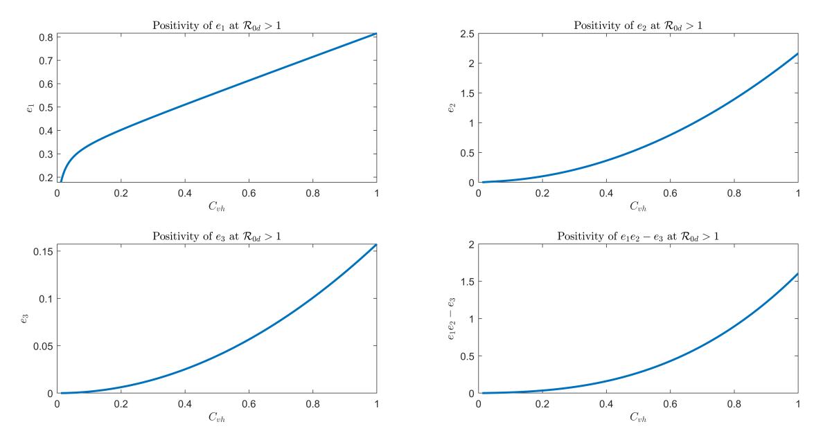
Figure 3: Numerical simulations for Routh-Hurwitz of \(\lambda^3 + e_1 \lambda^2 + e_2 \lambda + e_3\) at \(\mathcal{R}_{0d} > 1\).
Now, consider substituting \(E_3^{***}\) in \(\frac{dI_v}{dt} = 0\), and simplify with respect to the state variable \(I_v^{***}\), the resulting equation is given below
\[\frac{n_0(I_v^{***})^5 + n_1(I_v^{***})^4 + n_2(I_v^{***})^3 + n_3(I_v^{***})^2 + n_4I_v^{***} + n_5}{m_0(I_v^{***})^5 + m_1(I_v^{***})^4 + m_2(I_v^{***})^3 + m_3(I_v^{***})^2 + m_4I_v^{***} + m_5} = 0.\] (11)
See Appendix 3 for the coefficients of equation (11). This co-infection equilibrium does not have a closed analytical solution; consequently, we cannot conduct the stability analysis using the customary method used in the previous subsections. Instead, we will show the existence of the equilibrium. Thus, we have the following theorem.
Theorem 3.5 (Existence of COVID-19-Dengue Co-infection Equilibrium). The COVID-19-dengue co-infection equilibrium \(E_3^{***}\) exists if
\[0 < I_v^{***} < z_4\] and \(\mathcal{R}_{0c} > 1\), where
\[z_4 = \frac{N_h}{2C_{ch}} \left[ \sqrt{4\mu_h(\mu_h + \gamma_c)\mathcal{R}_{0c} + \gamma_c^2} - (2\mu_h + \gamma_c) \right]. \tag{12}\]
Proof: To show that the co-infection equilibrium point exists, we need to determine the threshold values of the parameters together with equation (11) such that all state variables must be
\[S_h^{***}, I_d^{***}, R_d^{***}, I_{dc}^{***}, I_c^{***}, R_c^{***}, I_{cd}^{***}, I_x^{***}, R_h^{***}, S_v^{***}, I_v^{***} > 0\]
since both diseases exist and persist in this equilibrium.
Now, consider the state variable \(S_h^{***}\), given as
\[S_h^{***} = \frac{(\mu_h + \gamma_c)N_h + C_{vh}I_v^{***}}{\beta}.\]
Then, \(S_h^{***}\) is positive if \(I_v^{***}>\frac{-(\mu_h+\gamma_c)N_h}{C_{vh}}\) for positive-valued \(C_{vh}\). Accordingly, it must be \(I_v^{***}>0\) to satisfy the nonnegativity of the solutions in Theorem 2.3. This condition also applies to \(I_d^{***}\), \(R_d^{***}>0\).
Similarly, for \(I_{dc}^{***}\), we need to show that this is positive, that is,
\[I_{dc}^{***} = \frac{\gamma_c C_{vh} \left[ \mu_h(\mu_h + \gamma_c) (\mathcal{R}_{0c} - 1) N_h^2 - (2\mu_h + \gamma_c) C_{vh} I_v^{***} N_h - (I_v^{***})^2 C_{vh}^2 \right] I_v^{***}}{\beta_c (\gamma_d + \mu_h) (C_{vh} I_v^{***} + N_h \mu_h) \left[ (\mu_h + \gamma_c) N_h + I_v^{***} C_{vh} \right]} > 0.\] (13)
The inequality (13) is true if we have the following values for \(I_n^{***}\)
\[I_{v}^{***} > 0, I_{v}^{***} > \frac{-N_{h}}{2C_{vh}} \left[ \sqrt{4\mu_{h}(\mu_{h} + \gamma_{c})\mathcal{R}_{0c} + \gamma_{c}^{2}} + 2\mu_{h} + \gamma_{c} \right], \text{ and}\] \[I_{v}^{***} < \frac{N_{h}}{2C_{vh}} \left[ \sqrt{4\mu_{h}(\mu_{h} + \gamma_{c})\mathcal{R}_{0c} + \gamma_{c}^{2}} - (2\mu_{h} + \gamma_{c}) \right].\] \[(14)\]
The intersection of the inequalities in (14) is shown by
\[0 < I_v^{***} < \frac{N_h}{2C_{vh}} \left[ \sqrt{4\mu_h(\mu_h + \gamma_c)\mathcal{R}_{0c} + {\gamma_c}^2} - (2\mu_h + \gamma_c) \right] = z_4,\] and this will be true only if \(\mathcal{R}_{0c} > 1\). Denoting the right-hand side of the inequality as \(z_4\). Thus, in this case, \(I_{dc}^{***} > 0\) if
\[\mathcal{R}_{0c} > 1\], and \(0 < I_v^{***} < z_4\). (15)
These conditions also apply to state variables \(I_c^{***}, R_c^{***}, I_{cd}^{****}, I_x^{***} > 0\). Moreover, we have \(R_h^{***} > 0\), since this co-infection state variable point is expressed in variables \(I_{dc}^{***}, I_{cd}^{***}, I_x^{***} > 0\). Furthermore, \(S_v^{***} > 0\) if \(I_v^{***} > 0\), that is, for \(\mathcal{R}_{0c} > 0\).
4. Numerical Simulation
This section presents numerical simulations of COVID-19 and dengue co-infections using Eulers approximation method, based on the parameter values outlined in Table 2. These simulations serve to validate the analytical results obtained earlier and offer insight into how different parameter values influence disease dynamics. By analyzing the impact of these parameters, the simulations provide practical inputs for policymakers seeking to develop strategies for disease containment and management of co-infections.
4.1. Model elasticity analysis
An elasticity analysis was conducted to assess how sensitive the basic reproduction number \(\mathcal{R}_0\) is to changes in various model parameters. This technique, adopted from [8] and [23], calculates the elasticity of \(\mathcal{R}_0\) with respect to a parameter p as
\[\chi_p^{\mathcal{R}_0} = \frac{\partial \mathcal{R}_0}{\partial p} \frac{p}{\mathcal{R}_0}.\] (16)
In practical terms, elasticity measures the percentage change in \(\mathcal{R}_0\) resulting from a 1% change in the parameter p. This analysis helps identify the parameters that most strongly influence disease transmission and control. A positive elasticity value depicts a direct proportional relationship between these parameters. Otherwise, when the index is negative, it describes an inverse relationship. Since \(\mathcal{R}_0 = \max{\{\mathcal{R}_{0c}, \mathcal{R}_{0d}\}}\), the analysis is performed separately as shown in Figure 4.
Parameters with high absolute-valued elasticity indices are critical for disease intervention, as they have the greatest influence on \(\mathcal{R}_0\). These parameters can be targeted for public health measures, such as vaccination programs or vector control strategies which can significantly reduce the spread of COVID-19, dengue, or their co-infection.
Model parameters \(\Lambda_h\), \(\beta_c\) for COVID-19's basic reproduction number \(\mathcal{R}_{0c}\), as well as \(\Lambda_h\), \(\Lambda_v\), \(C_{hv}\), \(C_{hv}\) for dengue's basic reproduction number \(\mathcal{R}_{0d}\), have positive elasticity indices. This indicates that increasing these parameters will lead to an increase in disease spread. Conversely, parameters \(\mu_h\), \(\gamma_c\), \(N_h\) for \(\mathcal{R}_{0c}\), and \(\mu_h\), \(\mu_v \gamma_d\), \(N_h\) for \(\mathcal{R}_{0d}\) have negative elasticity indices, meaning that increasing these values can help in reducing disease transmission. These findings highlight key targets for intervention, such as increasing recovery rates or reducing transmission coefficients through public health interventions.
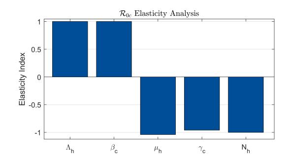
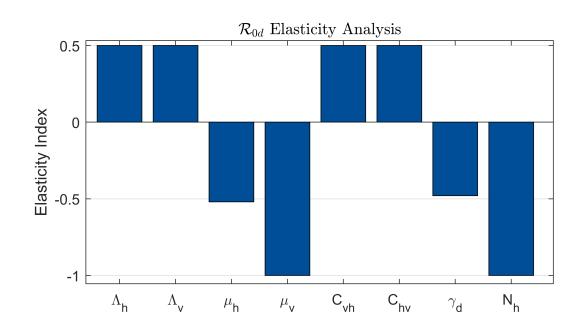
Figure 4: Elasticity analysis of the basic reproduction number \(\mathcal{R}_0\).
4.2. Stability and existence plots of equilibrium
This subsection presents the stability and existence regions for the identified equilibrium points using a phase diagram. The analysis uses varied values for the parameters \(\beta_c\) (COVID-19 transmission coefficient) and \(C_{vh}\) (dengue transmission coefficient from vector-to-human). These parameters are chosen due to their significant influence on disease transmission dynamics, as indicated by the elasticity analysis. The Monte Carlo numerical simulation method is employed to generate the phase diagram and verify the analytical results.
Figure 5 shows the six (6) distinct regions of the phase diagram and its equilibrium properties.
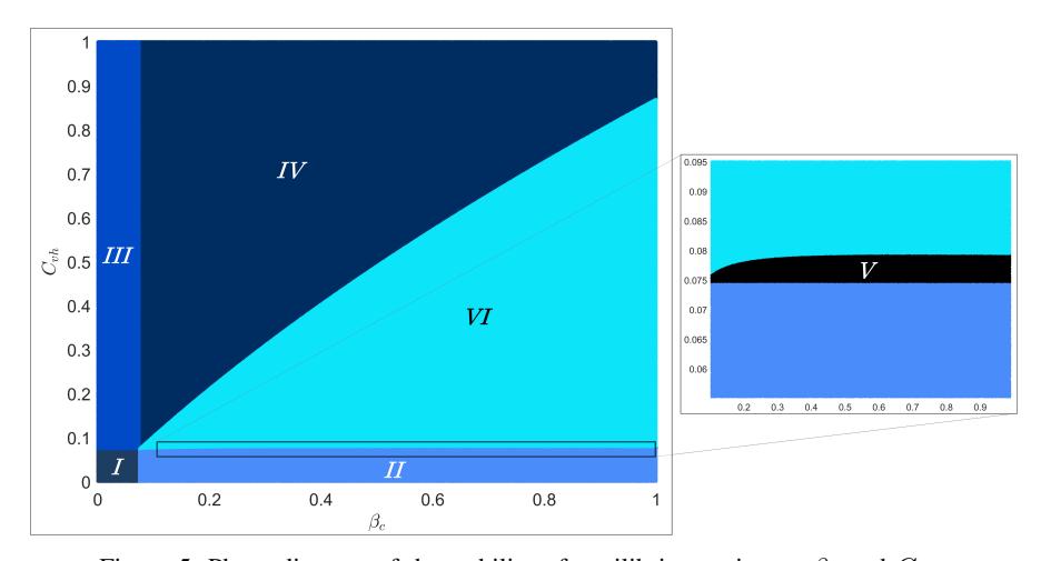
Figure 5: Phase diagram of the stability of equilibrium points at \(\beta_c\) and \(C_{vh}\).
\(I=E_0\) exists and is stable; \(II=E_0\) exists and unstable, \(E_1^*\) exists and is stable; \(III=E_0\) exists and unstable, \(E_2^{**}\) exists and is stable; \(IV=E_0\), \(E_1^*\) exist and unstable, \(E_2^{**}\) exists and is stable; \(V=E_0\), \(E_2^{**}\) exist and unstable, \(E_1^{*}\) exists and is stable; and \(VI=E_0\), \(E_1^{**}\), \(E_2^{**}\) exist and unstable, \(E_3^{***}\) exists.
4.3. Verification of analytical stability and existence of equilibrium points
Random \(\beta_c\) and \(C_{vh}\) values were selected from different regions in the phase diagram (Figure 5) to verify the stability and existence of equilibrium points. The numerical simulations confirm:
(Simulation 1) (0.0322284, 0.0407441) shows a stable Disease-Free Equilibrium \(E_0\);
(Simulation 2) (0.591375, 0.0772269) shows a stable COVID-19-only Equilibrium \(E_1^*\);
(Simulation 3) (0.324883, 0.589024) shows a stable Dengue-only Equilibrium \(E_2^{**}\); and
(Simulation 4) (0.546078, 0.277202) shows the existence of a stable Co-infection Equilibrium \(E_3^{***}\).
These simulations highlight the conditions under which each equilibrium can be achieved and maintained, providing insights into potential strategies for containing one or both diseases depending on the dominant transmission dynamics. Thus, the existence of a stable equilibrium suggests that the disease dynamics between COVID-19 and dengue will eventually settle into a predictable pattern which can inform long-term strategies for disease management among decision and policy makers.
Consider the population initial values of \(N_h(0) = 500000\), \(S_h(0) = 492450\), \(I_d(0) = 2000\), \(I_{dc}(0) = 300\), \(R_d(0) = 0\), \(I_c(0) = 5000\), \(I_{cd}(0) = 200\), \(R_c(0) = 0\), \(I_x(0) = 50\), \(R_h(0) = 0\), \(N_v(0) = 100000\), \(S_v(0) = 90000\), and \(I_v(0) = 10000\) and selected \(\beta_c\), \(C_{vh}\) values. The graphical results (see Figures 6 to 9), supported by the tabular values (see Tables 3 to 6), show the convergence of the simulation at t = 5000 days to their respective equilibrium points which are computed analytically.
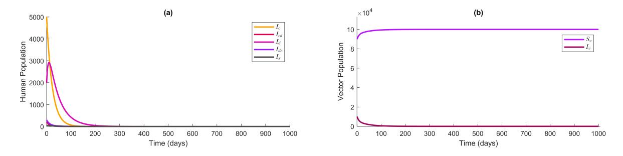
Figure 6: (Simulation 1) Disease-free equilibrium is asymptotically stable. (a) all disease-infected human compartments (zoomed). (b) vector compartments.
| Variable | \(E_0\) | \(E_1^*\) | \(E_2^{**}\) | \(E_3^{***}\) | Simulation |
|---|---|---|---|---|---|
| \(\overline{S_h}\) | 500000 | 1154704.72 | 802134.86 | 1154704.72 | 499999.99 |
| \(I_d\) | 0 | 0 | -12178.18 | \(4.89 \times 10^{-45}\) | \(2.95 \times 10^{-45}\) |
| \(R_d\) | 0 | 0 | -289956.68 | \(2.69 \times 10^{-43}\) | 0.004 |
| \(I_{dc}\) | 0 | 0 | 0 | \(-2.60 \times 10^{-45}\) | \(1.67 \times 10^{-53}\) |
| \(I_c\) | 0 | -26389.25 | 0 | -26389.25 | \(7.02 \times 10^{-89}\) |
| \(R_c\) | 0 | -628315.47 | 0 | -628315.47 | 0.002 |
| \(I_{cd}\) | 0 | 0 | 0 | \(-6.15 \times 10^{-45}\) | \(6.70 \times 10^{-97}\) |
| \(I_{x}\) | 0 | 0 | 0 | \(-2.21 \times 10^{-46}\) | \(3.46 \times 10^{-138}\) |
| \(R_h\) | 0 | 0 | 0 | \(-2.13 \times 10^{-43}\) | 0.0002 |
| \(S_{\bm{v}}\) | 100000 | 100000 | 113866.92 | 100000 | 100000 |
| I.,. | 0 | 0 | -113866.92 | \(-1.45 \times 10^{-11}\) | \(3.78 \times 10^{-45}\) |
Table 3: (Simulation 1) Simulation value converges to \(E_0\).
4.4. (Simulation 5) Effect of transmission rate \((\beta_c)\) and recovery rate \((\gamma_c)\) on COVID-19 infection, dengue infection, and COVID-19-dengue co-infection
The simulation shown in Figure 10, with \(C_{vh}=0.5\) and \(\gamma_d=1/14\), illustrates the impact of the COVID-19 transmission rate (\(\beta_c\)) and recovery rate (\(\gamma_c\)) on the duration and the spread of infection. This can be observed during the onset of the disease in the first wave. Interventions such as improving the recovery rate by reducing the recovery period from 21 to 10 days lead to a noticeable flattening of the epidemic curve in subsequent waves, even as \(\beta_c\) remains high. This demonstrates the effectiveness of timely interventions, such as accelerated recovery through early diagnosis and treatment, in mitigating the severity of outbreaks.
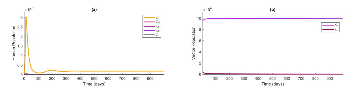
Figure 7: (Simulation 2) COVID-19-only equilibrium is asymptotically stable. (a) all disease-infected human compartments (zoomed). (b) vector compartments.
Table 4: (Simulation 2) Numerical simulation value converges to \(E_1^*\).
| Variable | \(E_0\) | \[E_1^*\] | \(E_2^{**}\) | \(E_3^{***}\) | Simulation |
|---|---|---|---|---|---|
| \(S_h\) | 500000 | 62928.41 | 484829.12 | 62928.48 | 62928.49 |
| \(I_d\) | 0 | 0 | 611.49 | 0.06 | 0.06 |
| \(R_d\) | 0 | 0 | 14559.40 | 0.19 | 0.20 |
| \(I_{dc}\) | 0 | 0 | 0 | 0.53 | 0.54 |
| \(I_c\) | 0 | 17617.09 | 0 | 17616.98 | 17616.98 |
| \(R_c\) | 0 | 419454.51 | 0 | 419438.88 | 419428.35 |
| \(I_{cd}\) | 0 | 0 | 0 | 0.05 | 0.06 |
| \(I_{x}\) | 0 | 0 | 0 | 0.04 | 0.04 |
| \(R_h\) | 0 | 0 | 0 | 14.78 | 25.28 |
| \(S_v\) | 100000 | 100000 | 99392.22 | 99999.41 | 99999.39 |
| \(I_{v}\) | 0 | 0 | 607.78 | 0.59 | 0.61 |
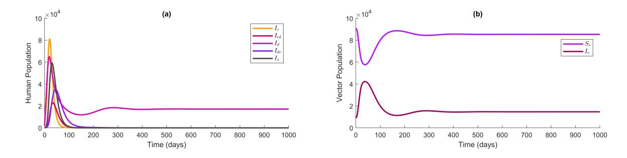
Figure 8: (Simulation 3) Dengue-only equilibrium is asymptotically stable. (a) all disease-infected human compartments (zoomed). (b) vector compartments.
Table 5: (Simulation 3) Numerical simulation value converges to \(E_2^{**}\).
| Variable | \(E_0\) | \(E_1^*\) | \(E_2^{**}\) | \(E_3^{***}\) | Simulation |
|---|---|---|---|---|---|
| \(S_h\) | 500000 | 114546.73 | 74027.33 | 141114.43 | 74027.33 |
| \(I_d\) | 0 | 0 | 17169.72 | 37595.66 | 17169.72 |
| \(R_d\) | 0 | 0 | 408802.94 | -404848.20 | 408802.82 |
| \(I_{\boldsymbol{dc}}\) | 0 | 0 | 0 | -12121.43 | \(2.39 \times 10^{-40}\) |
| \(I_c\) | 0 | 15536.50 | 0 | -14825.51 | \(1.33 \times 10^{-91}\) |
| \(R_c\) | 0 | 369916.76 | 0 | -52261.58 | \(7.51 \times 10^{-40}\) |
| \(I_{cd}\) | 0 | 0 | 0 | 52398.55 | \(1.14 \times 10^{-90}\) |
| \(I_{\boldsymbol{x}}\) | 0 | 0 | 0 | -8304.51 | \(1.22 \times 10^{-91}\) |
| \(R_h\) | 0 | 0 | 0 | 761252.60 | 0.13 |
| \(S_{\bm{v}}\) | 100000 | 100000 | 85346.28 | 79697.64 | 85346.28 |
| \(I_v\) | 0 | 0 | 14653.72 | 20302.36 | 14653.72 |
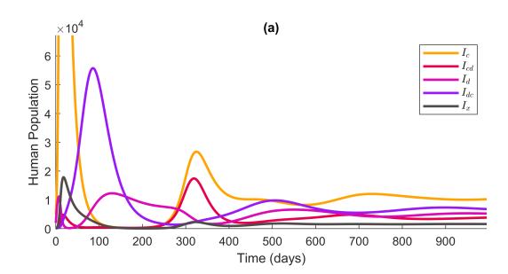
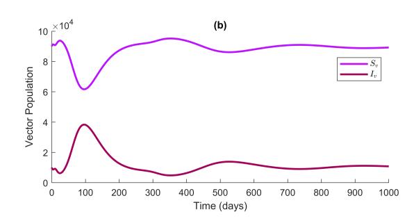
Figure 9: (Simulation 4) COVID-19-dengue co-infection equilibrium is asymptotically stable. (a) all disease-infected human compartments (zoomed). (b) vector compartments.
| Variable | \(E_0\) | \(E_1^*\) | \(E_2^{**}\) | \(E_3^{***}\) | Simulation |
|---|---|---|---|---|---|
| \(S_h\) | 500000 | 68148.30 | 153025.26 | 73457.12 | 73457.12 |
| \(I_d\) | 0 | 0 | 13985.55 | 4949.52 | 4949.52 |
| \(R_d\) | 0 | 0 | 332989.20 | 24178.40 | 24178.40 |
| \(I_{dc}\) | 0 | 0 | 0 | 6730.15 | 6730.15 |
| \(I_c\) | 0 | 17406.69 | 0 | 10641.35 | 10641.35 |
| \(R_c\) | 0 | 414445.01 | 0 | 86393.64 | 86393.64 |
| \(I_{cd}\) | 0 | 0 | 0 | 3775.46 | 3775.46 |
| \(I_{x}\) | 0 | 0 | 0 | 1601.84 | 1601.84 |
| \(R_h\) | 0 | 0 | 0 | 288272.53 | 288272.53 |
| \(S_{v}\) | 100000 | 100000 | 87730.42 | 89541.81 | 89541.81 |
| \(I_v\) | 0 | 0 | 12269.58 | 10458.19 | 10458.19 |
Table 6: (Simulation 4) Numerical simulation value converges to \(E_3^{***}\).
Moreover, as shown in [19], travel restrictions can lead to a significant decline in transmission rates, though the risk of new outbreaks may persist in areas with similar transmission potential.
On the other hand, we can observe an inverse relationship between the number of COVID-19 and dengue infections throughout the simulation. Whenever, \(\beta_c\) increases, the magnitude of dengue cases significantly declines during the first wave. This can be viewed as an inter-specific competition between the diseases. In addition, the occurrence of the COVID-19-dengue co-infection depends on the prevalence of both diseases. Whenever one of either disease dies out, the co-infection flattens its epidemiological curve.
4.5. (Simulation 6) Effect of transmission rate \((C_{vh})\) and recovery rate \((\gamma_d)\) on COVID-19 infection, dengue infection, and COVID-19-dengue co-infection
Figure 11 shows a simulation with \(\beta_c=0.3\) and \(\gamma_c=1/14\), illustrating that dengue prevalence increases significantly as the transmission rate \(C_{vh}\) (vector-to-human) rises. Reducing the transmission rate through minimizing mosquito-human effective contact rates (i.e. protection against mosquito bites [10]) and vector control measures (i.e. mosquito eradication programs), or by enhancing recovery rates (\(\gamma_d\)) through improved clinical management, can effectively shorten the duration of dengue outbreaks. Moreover, dengue vaccination indirectly reduces \(C_{vh}\) by lowering the number of infected individuals who can pass the virus to mosquitoes. This highlights the importance of targeting vector control alongside medical interventions to reduce dengue transmission. A similar inverse relation between COVID-19 and dengue was observed. Moreover, these case simulations resulted to approach different equilibrium solutions depending on the varied parameter values. If the prevalence of dengue is much greater than that of COVID-19, dengue will persist in the system, and vice versa. Hence, decision-makers may implement policies for stakeholders a combination of interventions, such as reducing disease transmission and improving recovery rates for both COVID-19 and dengue to mitigate its co-infection.
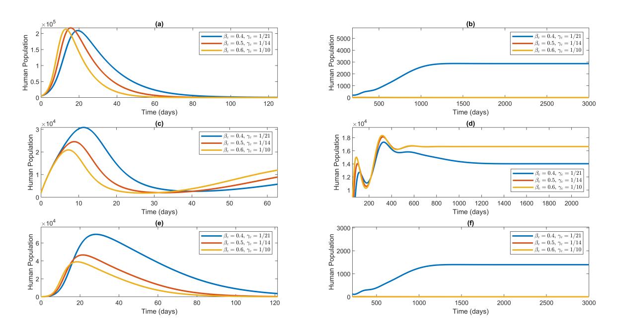
Figure 10: (Simulation 5) Effects of varying βc and γc values. (a) COVID-19 infection Ic first wave. (b) COVID-19 infection Ic succeeding outbreaks. (c) Dengue infection Id first wave. (d) Dengue infection Id succeeding outbreaks. (e) COVID-19-dengue infection Ix first wave. (f) COVID-19-dengue infection Ix succeeding outbreaks.
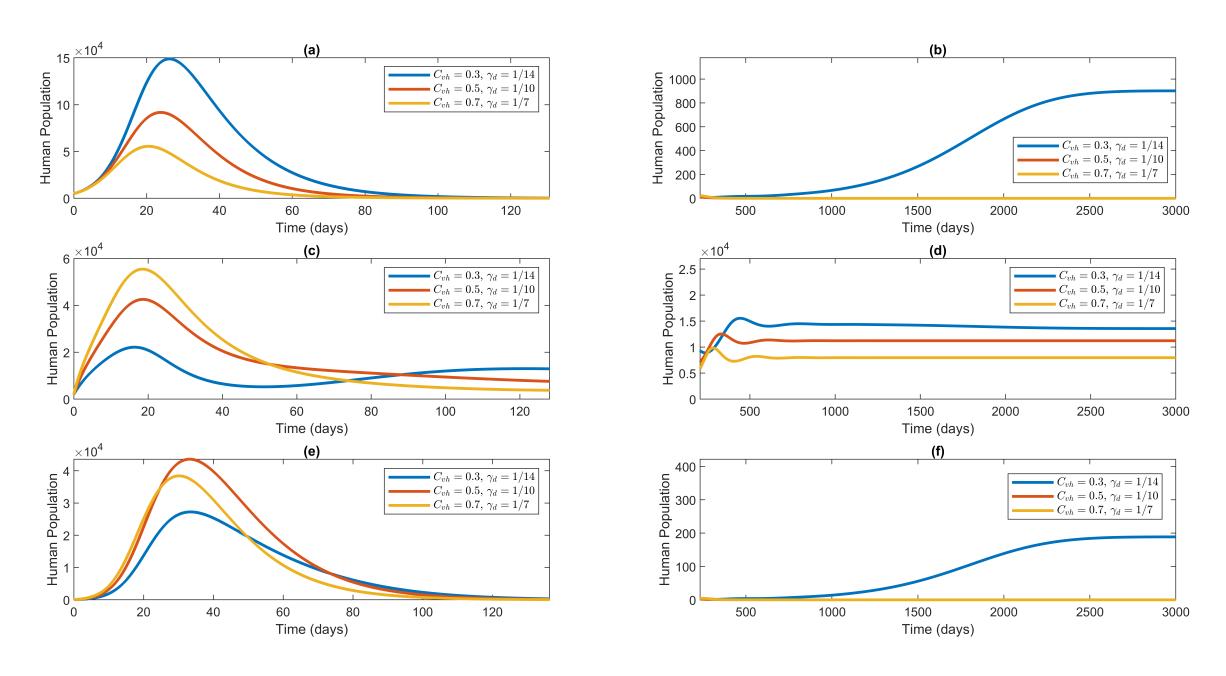
Figure 11: (Simulation 6) Effects of varying Cvh and γd values. (a) COVID-19 infection Ic first wave. (b) COVID-19 infection Ic succeeding outbreaks. (c) Dengue infection Id first wave. (d) Dengue infection Id succeeding outbreaks. (e) COVID-19-dengue infection Ix first wave. (f) COVID-19-dengue infection Ix succeeding outbreaks.
5. CONCLUSION
This study developed an 11-compartmentalized model to explore the transmission dynamics of COVID-19 and dengue co-infection. The well-posedness of the model was verified, ensuring the existence and uniqueness of its solutions based on continuity, local Lipschitz conditions, and invariance over a compact feasible region. These findings provide a robust mathematical framework for understanding how the two diseases interact in a population, offering valuable insights for shaping public health strategies aimed at managing co-infection which would potentially lead to policy formulation.
The basic reproduction number (R0) of the model was calculated using the NGM method. Four key equilibrium points were identified: the disease-free, COVID-19-only, dengue-only, and COVID-19-dengue coinfection equilibrium points. These equilibrium points provide critical insight into the conditions necessary for eradicating or controlling each disease, serving as a guide for developing phase-specific interventions during different stages of an epidemic or pandemic. Threshold values of the basic reproduction number were calculated to establish the conditions for the existence and stability of the equilibrium points. While an analytical solution for the co-infection equilibrium could not be derived, numerical simulations were employed to verify stability and explore the dynamics under different parameter conditions, providing valuable insights where analytical methods fall short.
An elasticity analysis was conducted to assess the sensitivity of the basic reproduction number (R0) to various model parameters, helping identify key factors influencing the spread of COVID-19 and dengue. Parameters with high elasticity, such as βc (COVID-19 transmission) and Cvh (dengue vector-to-human transmission), were used to construct a phase diagram via Monte Carlo simulations. These high-elasticity parameters are prime candidates for targeted interventions, such as public health campaigns aimed at reducing transmission rates or enhancing recovery through vaccination. The phase diagram depicts six distinct regions that describe the stability and existence of equilibrium points. These regions described different stable epidemiological scenarios whenever the parameter values were varied.
The numerical simulations provided valuable insights into the transmission dynamics of COVID-19 and dengue, with practical implications for policy formulation. These findings will be communicated to health authorities to inform the development of evidence-based policies aimed at controlling co-infections. Such policies may include enhanced disease surveillance, targeted vaccination campaigns, and vector control measures to mitigate the spread of both diseases, particularly in regions where co-infection poses a significant public health threat.
ACKNOWLEDGEMENT
Many thanks to the West Visayas State University - University Research and Development Center (WVSU-URDC) for funding this research study.